| Issue |
A&A
Volume 618, October 2018
|
|
|---|---|---|
| Article Number | A54 | |
| Number of page(s) | 15 | |
| Section | Galactic structure, stellar clusters and populations | |
| DOI | https://doi.org/10.1051/0004-6361/201832739 | |
| Published online | 12 October 2018 | |
Isochrone fitting in the Gaia era
1
Max Planck Institute for Solar System Research,
Justus-von-Liebig-Weg 3,
37077
Göttingen,
Germany
e-mail: This email address is being protected from spambots. You need JavaScript enabled to view it.
2
Stellar Astrophysics Centre, Department of Physics and Astronomy, Aarhus University,
Ny Munkegade 120,
8000
Aarhus C,
Denmark
Received:
31
January
2018
Accepted:
15
April
2018
Abstract
Context. Currently, galactic exploration is being revolutionized by a flow of new data: Gaia provides measurements of stellar distances and kinematics; growing numbers of spectroscopic surveys provide values of stellar atmospheric parameters and abundances of elements; and Kepler and K2 missions provide asteroseismic information for an increasing number of stars.
Aims. In this work, we aim to determine stellar distances and ages using Gaia and spectrophotometric data in a consistent way. We estimate precisions of age and distance determinations with Gaia end-of-mission (EoM) and Tycho-Gaia astrometric solution (TGAS) parallax precisions.
Methods. To this end, we incorporated parallax and extinction data into the isochrone fitting method used in the Unified tool to estimate Distances, Ages, and Masses (UniDAM). We prepared datasets that allowed us to study the improvement of distance and age estimates with the inclusion of TGAS and Gaia EoM parallax precisions in isochrone fitting.
Results. Using TGAS parallaxes in isochrone fitting, we are able to reduce distance and age estimate uncertainties for TGAS stars for distances up to 1 kpc by more than one third compared to results based only on spectrophotometric data. With Gaia EoM parallaxes in isochrone fitting, we will be able to further decrease our distance uncertainties by about a factor of 20 and age uncertainties by a factor of 2 for stars up to 10 kpc away from the Sun.
Conclusions. We demonstrate that we will be able to improve our distance estimates for about one third of stars in spectroscopic surveys and to decrease log(age) uncertainties by about a factor of two for over 80% of stars as compared to the uncertainties obtained without parallax priors using Gaia EoM parallaxes consistently with spectrophotometry in isochrone fitting.
Key words: stars: distances / stars: fundamental parameters / Galaxy: stellar content
© ESO 2018
1 Introduction
Understanding our Galaxy is essential to improving our understanding of the Universe. We can learn how the Galaxy was formed and how it has evolved by studying its current structure. To this end, stellar spectroscopic surveys that cover many stars are essential. These surveys provide data on stellar kinematics, chemical compositions, temperatures, and surface gravities. Another important ingredient for our understanding of galactic evolution are stellar ages (see, e.g., Martig et al. 2016; Amôres et al. 2017; Mackereth et al. 2017). For single stars, measuring ages remains a challenge, as the age of the star is only weakly related to parameters that we can observe (Soderblom 2010). We can compare an observed star with a set of models of stars of different ages and chemical compositions. Physical parameters of the model (or a range of models) with spectroscopic parameters that are close to those of the observed star will provide estimates of the physical parameters of this star. There exists a variety of methods using this approach, generally labelled “isochrone fitting”. The same method can be used to obtain absolute magnitudes of stars. These absolute magnitudes, combined with visible magnitudes from photometric surveys, can be used to derive values of distance and extinction in the direction of the star.
In Mints & Hekker (2017, hereafter Paper I) we presented a Unified tool to estimate Distances, Ages, and Masses (UniDAM) that uses isochrone fitting to estimate distances, ages, and masses for stars from spectrophotometric data. This tool was applied to a set of publicly available spectroscopic surveys, resulting in a catalogue of distances, ages, and masses for over 2.5 million stars. These results were released with the UniDAM source code1.
UniDAM is designed to be easily extendible to include new measurements. An important measure that was not included in UniDAM as provided in Paper I is parallax. In the current work, we introduce parallaxes into UniDAM and show the effect of parallax priors on the precision of age and distance estimates. For this we use parallax data from the Gaia catalogue. The released Gaia data (Gaia DR1; Lindegren et al. 2016) contain parallaxes and proper motions for 2.5 million stars in the Tycho-Gaia astrometric solution (TGAS) sample (Michalik et al. 2015). The upcoming Data Release 2 (DR2; see Katz & Brown 2017) will contain data with orders of magnitude increase in number of stars and in the precisions of the determined proper motions and parallaxes. Although far from being final, values of parallax and proper motions will have uncertainties not much higher than those predicted for end-of-mission (EoM) performance. These data will be complemented with data from Gaia radial velocity spectrometer (Recio-Blanco et al. 2016) and from ground-based spectroscopic surveys. This will include radial velocities and stellar physical parameters such as temperature, surface gravity, and chemical composition for millions of stars and will provide an unprecedented view of the Galactic structure and kinematics.
As we show in this work, for a large fraction of stars in spectroscopic surveys, distance will be almost entirely defined by parallax. Parallax does not, however, provide any other stellar parameters, and spectroscopic (or photometric) measurements are required to derive physical properties of stars. In Paper I we have shown that distance modulus and age estimates are correlated. Therefore, it is important to estimate distance and age consistently, to avoid biases.
Here wepresent the results of incorporating Gaia parallax data into UniDAM For other works that use Gaia data for isochrone fitting see, for example, McMillan et al. (2018) and Queiroz et al. (2018). Our work is novel in two ways. We demonstrate what precisions in distances and ages to expect with Gaia EoM parallax precisions. On top of that, for stars in the catalogue from Paper I that have TGAS counterparts, we publish updated distance and age estimates.
If parallax priors are used in isochrone fitting, the impact on the distance estimates is straightforward. For the large fraction of stars in the spectroscopic surveys, the distance will be primarily defined by their parallax. However, the uncertainty σd in distance d obtained from the parallax increases with distance: approximately as σd ≈ σπd2, where σπ is the parallax uncertainty. The uncertainties in distances derived from spectrophotometric data are much less sensitive to the distance itself. Therefore, the contribution of spectrophotometric data becomes more relevant for more distant stars.
The impact of parallax priors on derived ages is not straightforward. Gaia parallaxes combined with visible magnitudes and extinction values constrain the absolute magnitudes in different photometric bands for a given star. This adds constraints on the models used to fit the star. If consistent with other data, these constraints reduce the range of physical parameters covered by fitting models and thereby may reduce the uncertainty of estimates of parameters. As we show in thiswork, with TGAS data we improve the precision of age estimates for stars within 1 kpc from the Sun, as compared to results from Paper I. We also predict improvements in the precision of ages for stars with distances up to 10 kpc based on predicted parallax precisions of Gaia DR2 and future data releases. There is however a lower limit on the precision with which we can determine stellar age even in the case of the small parallax uncertainty that we expect from Gaia DR2. This is caused by the possibility that there is a range of models with different ages and spectroscopic parameters that fits into a narrow range of absolute magnitudes, dictated by parallax.
Along with this paper, we publish an updated version of UniDAM2 and the catalogue of updated distance, age, and mass estimates for over 400 000 stars from TGAS
2 Inclusion of parallax priors into UniDAM
In this section we provide a brief description of the method applied in the original version of UniDAM (see Paper I for more details). We subsequently show how Gaia parallaxes can be incorporated in a consistent manner into UniDAM
2.1 Age and distance measurements without parallax
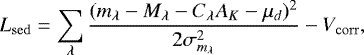
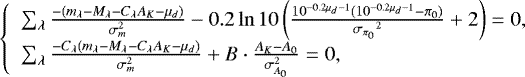
UniDAM, presented in Paper I, utilises a Bayesian method of deriving stellar parameters from spectrophotometric data. By comparing observed stellar parameters (Teff, logg, and [Fe/H]) and visible infra-red magnitudes (mλ) to spectral parameters and absolute magnitudes (Mλ) from PARSEC models (Bressan et al. 2012), we derived probability density functions (PDFs) for log(age), mass, distance modulus μd, and extinction in 2MASS K-band AK for a star.
In Paper I we showed that each model contributes a delta-function to the log(age) and mass PDFs for a given star. The contribution of each model to distance modulus and extinction PDFs has a bivariate Gaussian shape as the goodness-of-fit Lsed of the spectral energy distribution (SED) is quadratic in μd and AK:
 (1)
(1)
where mλ is the observed visible magnitude with the corresponding uncertainty  ; Mλ is the absolute magnitude of the model, and Cλ represents extinction coefficients. The summation is done over filters λ, for which photometry is available. The last summand Vcorr is the volume correction, introduced to compensate for the fact that with a given field of view we probe a larger volume at larger distances. Volume correction is expressed as a natural logarithm of the square of the distance, which is in turn expressed here through distance modulus μd:
 (2)
(2)
We refer the reader to Paper I for more discussion of volume correction and its effect on log(age) and distance modulus estimates.
The location of the Gaussian contribution of each model to the PDFs in distance modulus μd and extinction AK is calculated as optimal values (designated as  and
and  ) that minimise the goodness-of-fit Lsed (1) for this model. The width of the above Gaussian in distance modulus is
 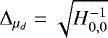 and in extinction
 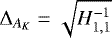 , where Hi,j is the Hessian matrix:
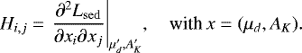 (3)
(3)
Substituting Eqs. (1) into (3), we obtain
 (4)
(4)
An important property of H, and therefore of  and
and  , is that they depend exclusively on the photometric uncertainties
  and extinction coefficients Cλ, and therefore are the same for all models of a given star. This means that Gaussian components contributed by each model to the PDFs for a given star have exactly the same shape and differ only by location. It is therefore possible to build PDFs in distance modulus and extinction by taking the distribution of
  and
and  , that is, the optimal values that minimise Lsed for each model. These distributions should be smoothed with Gaussian kernels of width
  for the distance modulus μd and
  for extinction AK, to account for the width of the Gaussians contributed by each model. This smoothing is, however, only a minor correction, because
  and
and  are an order of magnitude smaller than the width of the distribution of
  and
and  , as shown in Paper I.
The approach described above allows for production of PDFs in distance modulus and log(age) for stars for which spectrophotometric data are available. When Gaia parallaxes are available, this method has to be modified slightly. Below, we show how parallax data can be incorporated into UniDAM.
2.2 Age and distance measurements with parallax
In the current work we aim to improve stellar parameters determined by UniDAM by incorporating Gaia parallax data, in addition to effective temperature Teff, surface gravity logg, metallicity [Fe/H], and visible magnitudes mλ. This requires, as we show below, the use of an external value of the extinction.
Including parallax information into isochrone fitting is not trivial. The transformation from parallax uncertainties to distance uncertainties is non-linear; symmetric parallax uncertainties correspond to asymmetric distance uncertainties (Kovalevsky 1998; Astraatmadja & Bailer-Jones 2016). The asymmetry increases with increasing fractional parallax uncertainties. However, in the current work we show that asymmetries caused by transformation from parallax to distance uncertainties can be neglected in the majority of cases.
2.2.1 The need for an extinction prior
Constraints on stellar parameters can be degenerate for a star with a known parallax and unknown extinction. This is caused by the fact that the optimal values  and
and  which minimise Lsed in Eq. (1) are highly correlated. The aim of the parallax prior is to select models that give a matching
  and remove other models from the consideration, thus reducing the uncertainties in the measured parameters. However, due to correlations between
  and
and  , this cannot be achieved without a prior on extinction. This can be illustrated with the following example. Let us assume that we have two models for which minimising Eq. (1) (in other words, not using parallax data) results in optimal distance modulus and extinction values μ1, A1 and μ2, A2, with μ1 ≠ μ2. Now let us assume that we know that μ = μ1 from parallax measurement (μ1 = −5(log10π + 1), where π is the measured parallax). If we use this without a prior on extinction, we will still obtain two solutions μ1, A1 and
  . Due to the correlation between
  and
and  ,
,  will not be much larger than Lsed(μ2, A2), and the contribution of the second model to PDFs in all parameters will not be removed. Effectively a difference in distance modulus between models will be shifted into a difference in extinctions. To avoid this degeneracy, we need to put a prior on extinction AK.
2.2.2 Incorporating parallax and extinction into UniDAM
To incorporate priors on parallax and extinction, we modified the Lsed goodness-of-fit in Eq. (1). We added two priors, namely a prior on parallax:
 (5)
(5)
where π0 and  are measured parallax and its uncertainty. For a prior on extinction, we use the following expression:
 (6)
(6)
where A0 and  are measured extinction in K-band and its uncertainty taken from an extinction map. Effectively this prior allows AK to vary between zero and A0, and penalises larger values. We chose this form because A0 is the value of extinction at infinity, and we need to allow for lower extinctions for nearby stars. Three-dimensional (3D) extinction maps (e.g. Green et al. 2018) can be used to obtain more realistic prior Pr(AK), however these maps do not yet cover the whole sky, so cannot be applied to all surveys. The prior will be updated in future versions of UniDAM, when Gaia-based extinction maps become available.
If we take parallax to be  and extinction to be
  , we can define the new goodness-of-fit for the model as a function of μd, AK and parallax π, which in turn is a function of μd:
 (7)
(7)
Here, we add two quadratic terms for the extinction and parallax. This is done under the assumption that the uncertainties in these values have a normal distribution. Again, we can find optimal values of distance modulus  and extinction
  that minimise Lsed. The method of finding
  and
and  is given in Appendix A. The term containing parallax Pr(π) in Eq. (7) can be expressed as a function of distance modulus μd as:
 (8)
(8)
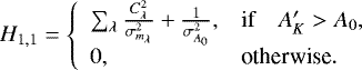
Therefore, the re-defined Lsed is no longer a quadratic function of μd and  is not constant for a given star. Instead, it is a function of the optimum parallax π′ for a given model:
 (9)
(9)
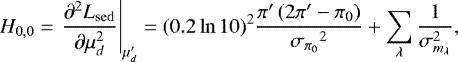
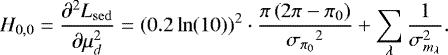
where 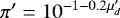 . The value of H1,1 will also change to:
 (10)
(10)
Thus H1,1 remains constant for all models with  and zero for models with
  . Therefore, the assumption made in Paper I that the PDF in μd and AK is a Gaussian with the same width for each model for a given star is no longer valid. This means that, formally, we have to calculate PDFs in distance modulus and extinction for each model by directly evaluating Eq. (7) over the two-dimensional (2D) grid. However, we argue that in many cases the contribution of each model to the PDF is still close to being Gaussian, and that H0,0 is nearly constant, so we can keep the approach introduced in Paper I. To illustrate this, we consider two regimes:
“photometry dominated”, where the fractional parallax uncertainty is large (
 ). In this case the location of the minimum of Lsed and the shape of Lsed around this minimum are defined primarily by the photometric components. This is because the first summand in Eq. (7) is much more sensitive to variations of μd than the third summand (parallax part). At the same time, the effect of the first summand in H0,0 (see Eq. (9)) is negligible, and Lsed is nearly quadratic in μd and AK. Thus, in case fractional parallax uncertainty is large, parallax can be considered as a minor correction to the method without the inclusion of parallaxes (see Sect. 2.1);
“parallaxdominated”, where the fractional parallax uncertainty is small (
 ). In this case the location of the minimum of Lsed is defined by the parallax component (see Eq. (7)).
If the optimal parallax π′ derived for each model is not close to π0, the parallaxterm in Eq. (7) will be large, making the overall goodness-of-fit large, that is Lsed ≫ 1. The contribution of the model to the PDF depends on Lsed: models with large Lsed typically contribute little to the PDF if there are other models with much smaller Lsed. If there are no models with a muchsmaller Lsed, then the overall fit for the star under consideration is bad. Therefore, we can assume that optimal parallaxes π′ derived for each model are all very close to π0.
As long as the optimal parallax value π′ is close to π0, we can approximate π′ by π0 in Eq. (9), such that H0,0 depends only on π0 and  and therefore is a constant for all models for a given star. In this “parallax dominated” case, we observed that
  computed from the Hessian matrix H is comparable to the scatter of optimal
  for all models. Therefore, the impact of smoothing the PDF in distance modulus with Gaussian kernel of width
  is no longer a minor correction and has to be accounted for. We can use the fact that for a given star, each model’s contribution is close to a Gaussian, the shape of which is defined by
  , π0 and
  and is the same for all models. Therefore, it is still valid to calculate the optimal
  and
and  for each model and then smooth the resulting PDFs with
  and
and  .
.
With the precision of spectrophotometric data that we have for our surveys, these two regimes overlap; there is a range of parallaxes for which photometry dominates the goodness-of-fit Lsed and fractional parallax uncertainty is small enough, so that π′ can be replaced by π0 in H0,0. To further understand these intermediate cases, we provide a more elaborate explanation of the properties of Lsed and H0,0 in Appendix B.
With the addition of parallax and extinction priors, we further constrain the stellar models that match the observations. In some cases, these priors are not consistent with spectrophotometric data. This can result in an increase in Lsed for models used to build the PDFs, which itself results in the broadening of PDFs of all parameters, including log(age) and distance modulus. A consequence of this is the increase in the uncertainties in the derived parameters. This also decreases the best-model probability pbest introduced in Paper I. Low values of pbest generally indicate disagreement between constraints based on spectroscopy, photometry, parallax, and extinction.
3 Applications of the modified UniDAM
The goals of this study are first, to provide an indication of the precision with which age and distance can be determined using Gaia EoM parallaxes and uncertainties and second, to re-derive distances and ages of stars for which TGAS parallaxes are available. To achieve the latter goal, we cross-matched all spectroscopic surveys used in Paper I with TGAS, and run the updated UniDAM including parallax and extinction priors on the stars for which TGAS parallaxes are available. Table 1 shows the number of TGAS stars contained in different surveys (see Paper I for a discussion of survey properties and quality cuts). The middle panels in Figs. 1 and C.1 show the number of stars in the complete survey and in the TGAS overlap as a function of measured distance modulus. For most surveys, only a small fraction of all stars have a TGAS counterpart and these stars are closer on average. The exception is GCS, for which some nearby stars were not included in TGAS, because they were above the brightness limit of TGAS. As in Paper I, we include GCS in our sample, although it is a photometric survey. In GCS, narrow-band photometry is used to derive stellar parameters (Teff, logg, and [Fe/H]) with precisions comparable to those obtained with low-resolution spectroscopy.
In addition to the data used in Paper I, we added recently released LAMOST DR33 and TESS-HERMES DR1 (Sharma et al. 2018). For the APOGEE survey, we switched to using DR14 (Abolfathi et al. 2018). As before, 2MASS and AllWISE photometry was used. Small overlap with TGAS for most surveys is caused by the fact that TGAS contains primarily bright stars. There is no overlap between SEGUE (Yanny et al. 2009) and TGAS and we estimate only what can be achieved with Gaia EoM parallaxes for this survey. About one quarter of SEGUE stars have no 2MASS or AllWISE counterpart, and therefore there is no photometry that can be used in UniDAM4. These sources were excluded from analysis. With deep spectroscopic surveys like SEGUE, LAMOST GAC, and Gaia-ESO, we will have to wait for later Gaia data releases to obtain parallaxes for the majority of stars.
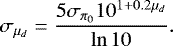
We chose a prior on extinction as defined in Eq. (6). For this prior, we took the mean value A0 from Schlegel map (Schlegel et al. 1998). This map has a resolution of approximately 0.1 degree. The variance of the extinction  for a given map cell was calculated as a variance of extinction values within one degree from the centre of that cell.
The primary goal is to show what to expect in terms of age and distance modulus precisions when using parallax priors with Gaia EoM precisions. For this, we simulated Gaia EoM data by taking parallax values from the TGAS or UniDAM catalogue and assigning Gaia EoM parallax uncertainties to these parallaxes. The distributions of uncertainties for distance and log(age) values derived using these simulated data are representative for what we expect to obtain with Gaia EoM data. Henceforth, we can estimate precisions with which ages and distances can be determined.
Overall, for each of the spectroscopic surveys, we compiled five datasets as follows:
- 1.
Complete data of spectroscopic survey without parallaxes – these are the same data as presented in Paper I.
- 2.
Subset of dataset 1, containing only sources that have a TGAS counterpart. For this dataset no parallax information was used.
- 3.
As in dataset 2, now using parallax data from TGAS
- 4.
As in dataset 3, now with parallax uncertainties as they are expected to be at the end of the Gaia mission according to the Gaiascience performance guide5, namely:
 (11)
(11)Here, mG is visible magnitude in Gaia optical G-band.
- 5.
As in dataset 1, extended with parallaxes already obtained by UniDAM and assuming parallax uncertainties as they are expected to be at the end of the Gaia mission (see Eq. (11)). For stars in the spectroscopic survey, the overlap with Gaia DR1 is used to extract values of mG. These values are substituted into Eq. (11) to calculate Gaia EoM parallax uncertainty. There is a small (typically less than 3%) fraction of stars in each spectroscopic survey that does not have a counterpart in Gaia DR1 and these stars are not included in this dataset. We consider this difference in the sample of stars in dataset 1 and this dataset negligible for our purposes. We note that as the number of stars released in Gaia DR2 is expected to grow from 1.1 to 1.5 billion (Katz & Brown 2017), we expect that the fraction of stars in spectroscopic surveys without Gaia counterpart will further decrease.
Summarising, datasets 1 and 2 represent data without prior parallax information, dataset 3 represents data with the current state-of-the-art TGAS parallaxes and datasets 4 and 5 simulate Gaia EoM parallax precision. The last two datasets aim at demonstrating the improvements in the precision of age and distance that can be expected from including priors from parallaxes with Gaia EoM precision.
Among datasets that include parallax data with Gaia EoM precision, dataset 4 has the advantage of having precise TGAS parallaxes, while dataset 5 contains a larger number of stars covering a large range in parallaxes, which better represents the content of Gaia EoM data. As compared to the TGAS sample, this dataset contains more faint stars, for which Gaia EoM parallax uncertainty will be higher. Consequently, we expect distance and age uncertainties for all stars in a certain distance bin to be higher for dataset 5 than for dataset 4. In the last paragraph of Sect. 2.2.2, we discussed that the addition of Gaia parallax and extinction values can lead to higher uncertainties in derived distance and age, in case the constraints provided by parallax and extinction priors and the spectrophotometric constraints are not consistent. Parallaxes used in dataset 5, however, are taken from UniDAM output for dataset 1, and not from Gaia. Therefore, the uncertainties derived for dataset 5 are in the limit of no mismatch between parallax constraints. Nevertheless, there can be a disagreement between extinction prior and constraints on extinction from spectrophotometric data, which can lead to higher uncertainties.
Following Eq. (11), fainter stars will have larger parallax uncertainties and therefore larger uncertainties in the derived distances. Age uncertainty is also sensitive to stellar brightness, however in a less direct way: fainter stars typically have larger uncertainties in visible magnitudes and lower signal-to-noise ratio (S/N) of observed spectra, and therefore larger uncertainties in spectroscopic parameters. Additionally, age uncertainty depends much more on the location of a star in the Hertzsprung–Russell diagram, due to the different rate of changes in Teff and logg during different stages of stellar evolution. For example, during the main sequence evolutionary stage, Teff and log g of a star are nearly constant, while around the turn-off point, Teff changes rapidly, and on the red giant branch, logg changes rapidly. Therefore, the median measured age precisions for each dataset depend directly on the distribution of stars in that dataset. This implies that only datasets containing the same stars can be directly compared. Therefore, dataset 1, containing all survey stars, can only be directly compared to dataset 5 (here we neglect the small difference in the number of stars between datasets 1 and 5); and dataset 2, containing only the TGAS overlap, can only be directly compared to datasets 3 and 4.
Total number of sources and TGAS overlap for different surveys.
4 Results and discussion
We apply the updated UniDAM, as described in Sect. 2.2, to all datasets for each spectroscopic survey presented in Sect. 3. We publish the results for dataset 1 for new surveys (TESS-HERMES, Sharma et al. 2018; LAMOST DR3, Luo et al. 2015; and APOGEE DR14; Abolfathi et al. 2018); thus extending the number of stars in our catalogue, as compared to the catalogue in Paper I, to nearly 4 million stars. We also publish results for dataset 3 for all surveys along with this paper. These results contain improved log(age) and distance estimates for about 400 000 stars.
In this section we compare the precision of distance modulus and log(age) for different datasets. The quantitative behaviour of the relation of distance modulus uncertainty to distance modulus in all surveys depends on the content of each dataset for each spectroscopic survey; therefore, we list and discuss our results for every dataset for each survey. We first consider distance modulus precision in Sect. 4.1 and then proceed to log(age) precision in Sect. 4.2.
4.1 Distance modulus precision
Distance modulus precision is closely related to parallax precision: for a value of parallax uncertainty  , the corresponding distance modulus uncertainty
  is a function of distance modulus μd and can be expressed as:
 (12)
(12)
The above equation is valid only approximately, as the distance modulus uncertainties become asymmetric when propagated from the symmetric parallax uncertainties (see Kovalevsky 1998; Astraatmadja & Bailer-Jones 2016). From Eq. (12), it follows that the distance modulus uncertainty depends on two values: first, the parallax uncertainty, and second, the value of the distance modulus itself. For Gaia EoM, parallax uncertainty estimates depend on visible magnitudes for stars fainter than 12m in G-band (see Eq. (11)). The distance modulus uncertainty derived from spectrophotometric data is much less sensitive to visible magnitudes. Once a star is bright enough to be accessible to spectrophotometric observations, uncertainties in the measured parameters, and thus the derived distance uncertainty, will not depend directly on the distance. Therefore, we can expect that for distant stars (with μd ≳ 15m) the spectrophotometric data constrain the distance modulus more than parallax data. Thus, the benefits of using the parallax priors for surveys containing primarily nearby stars (like GCS and TESS-HERMES) will be higher than those for deep surveys containing distant stars, which are fainter on average. For deep surveys, like APOGEE, SEGUE, and LAMOST and future surveys like 4MOST (de Jong et al. 2016) and WEAVE (Dalton et al. 2014), there will be a high percentage of stars for which spectrophotometric information will improve distance modulus uncertainties.
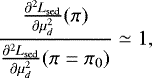
The toppanels of Figs. 1 and C.1 show median distance modulus uncertainties  as functions of measured distance modulus μd. The results for dataset 3 show that the use of TGAS parallaxes provides a substantial improvement in the precision of distance modulus estimation as compared to dataset 2, which contains the same data without parallaxes, for distance moduli up to μd = 10m.
For illustrative purposes and to better understand what limits the distance modulus uncertainty, we produced two approximations for the  function; these are shown in the top panels of Figs. 1 and C.1 with black dashed and dotted lines. The first approximation F1 (μd) is obtained using Eq. (12) to propagate 10−5 arcsec parallax uncertainties expected for stars brighter than mG = 12m (see Eq. (11)) to distance modulus uncertainties. This provides an approximation of the resulting precision when TGAS parallaxes are used with Gaia EoM parallax precisions (dataset 4), because almost 90% of TGAS stars are brighter than mG = 12m. This approximation is indeed representative of the measured precision, except for the most distant (μd > 15m) bins in the RAVE surveys: at these distances, measured parallax values become close to typical parallax uncertainty for RAVE stars (10−5 arcsec) and spectrophotometric constraints improve distance estimations.
When parallax values are taken from UniDAM and parallax uncertainties are taken from Gaia EoM uncertainty prediction (dataset 5), the above approximation does not work, because for stars in that dataset that are fainter than mG = 12m, the parallax uncertainty will be larger than 10−5 arcsec. To produce an approximation for these cases, we took μd as derived by UniDAM for each star and additionally calculated  using Eq. (11) and visible magnitude mG from Gaia DR1. Values of
  were then propagated to distance modulus uncertainty using Eq. (12). We then obtained the mean distance modulus uncertainty as a function of distance modulus. The resulting function F2 (μd) is shown in Figs. 1 and C.1 with black dashed lines.
To illustrate how results for dataset 5 compare with parallax-only approximation F2 (μd) and results for spectrophotometry-only dataset 1, we can define three distance ranges of interest:
Range A: “parallax dominated”, where distance modulus is almost entirely defined by parallax. We define it as a range where the improvement in the distance modulus uncertainty for dataset 5 is less than 10% as compared to our approximation F2.
Range B: “intermediate”, where distance modulus is improved by the use of parallax. We define it as a range that spans from the upper limit of the range A to the point where the improvement in the distance modulus uncertainty for dataset 5 is less than 10% as compared to the dataset 1 (in which only spectrophotometric data is used).
Range C: “spectrophotometry dominated”, where parallax has almost no influence on distance modulus uncertainty. We define it as a range where the improvement in distance modulus uncertainty for dataset 5 is less than 10% as compared to the dataset 1 (in which only spectrophotometric data is used).
These ranges are labelled in the top panels of Figs. 1 and C.1 with large letters A, B, and C. Range borders are marked with vertical grey lines.
In Table 2 we show fractions of stars in each survey that fall into ranges A, B, and C, as well as locations of range borders. These fractions depend on the distribution of stars in both visible and absolute magnitudes and are therefore very different from survey to survey. For GALAH, GCS, RAVE, RAVE-on, and TESS-HERMES, the majority (over 95%) of stars fall into range A, where Gaia parallaxes define the distance modulus. For other surveys, spectrophotometric constraints play a role for a large portion of stars: for LAMOST-based surveys, Gaia-ESO and APOGEE, 20–80% of stars are in range B, which means that spectrophotometry constraints give at least 10% improvement over pure-Gaia distances. Range B extends from distance modulus of approximately 11m to 16m, or from 1.5 to 15 kiloparsecs. A large portion of stars is in range C for Gaia-ESO (6%), APOGEE (7%), and SEGUE (37%). This means that Gaia parallax will give almost no improvement in distance modulus for these stars. Also, for SEGUE, only a few stars are in range A. This is because SEGUE stars are faint, and Gaia parallax uncertainties will be higher for them than for stars in other surveys. We expect for future surveys to contain a large portion of stars in ranges B and C, and therefore we will need a combination of spectrophotometric data and Gaia parallaxes to derive best possible distance estimates for them.
In Table 3 we give another view on results by listing the median uncertainty per dataset for each survey.The first section of Table 3 shows median distance modulus uncertainties for each dataset for each spectroscopic survey. Datasets 1 and 2 are built using only spectrophotometric data, and the small difference between median uncertainty values for these datasets is caused by the fact that stars in TGAS overlap are typically brighter. For these stars, input spectrophotometric parameters are generally more precise than those for fainter survey stars at the same distance, and therefore distance modulus and log(age) uncertainties are smaller.
The useof TGAS parallaxes for dataset 3 increases the precision in the distance modulus by about one third. The exception here is GCS, for which TGAS parallaxes increase distance modulus precision by almost a factor of five. This is caused by the fact that GCS contains nearby HIPPARCOS stars, for which parallaxes in TGAS have high precision.
For datasets 4 and 5, which are constructed using expected Gaia EoM parallax precisions, the median distance modulus uncertainties are on the orderof 0. m1 or even 0. m01. The actual value depends primarily on the distance distribution of stars in the spectroscopic survey which means that for deeper surveys, parallax uncertainties will be larger, leading to larger distance modulus uncertainties. Similarly, in comparison to dataset 4, dataset 5 contains more distant stars that are fainter on average. Therefore, median distance modulus uncertainties for dataset 5 are in most cases larger than those for dataset 4.
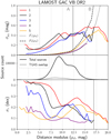 |
Fig. 1 Distance modulus uncertainties |

Ranges of distance modulus μd improvement from the use of Gaia end of mission parallax priors.
4.2 log(age) precision
The effect of the parallax priors in UniDAM on the log(age) uncertainty is presented in the lower panels of Figs. 1 and C.1 and in Tables 3 and 4. This effect is not straightforward to quantify. Parallax data constrain the absolute magnitude of the star, which can have an impact on the log(age) estimate. This improvement varies along the Hertzsprung–Russell diagram, with improvements being larger for lower main sequence stars, and smaller or close to zero for the main sequence turn-off region. In the turn-off region, age depends less on absolute magnitudes and more on temperature; therefore, little or no further improvement of log(age) estimates can be made by adding parallax data.
The decrease in log(age) uncertainties with distance modulus that is present in some surveys is caused by the fact that log(age) uncertainties are much higher for lower main sequence stars than for turn-off stars and giants. At the same time, at a given distance, main sequence stars are harder to detect than giants, because they are intrinsically fainter. This causes the fraction of observed main sequence stars per distance modulus bin to decrease with distance modulus. Hence, the median log(age) uncertainty per bin also decreases with distance modulus. For APOGEE and LAMOST-Cannon surveys, which preferentially contain giants, this decreasing trend is absent.
With Table 4 we illustrate where we can improve log(age) uncertainties by using TGAS and Gaia EoM parallaxes. We do this by calculating the maximum distance at which the parallax prior has almost no influence on log(age) uncertainty. We define this for the TGAS sample as a range where the uncertainty for datasets 3 is smaller than 90% of the uncertainty for dataset 2 (in which only spectrophotometric data are used). Similarly, for Gaia EoM parallaxes, we compare datasets 5 and 1. In both cases, we provide the fractions of stars that are within the listed ranges. In the bottom panels of Figs. 1 and C.1, we show with a vertical grey line the maximum distance modulus for which log(age) uncertainty for dataset 5 is smaller than 90% of the uncertainty for dataset 1 (see fourth column of Table 4). For GCS, the improvement in log(age) is more than 10% for all stars, and this survey is therefore not listed in Table 4. We observe log(age) estimate improvements from the use of TGAS parallaxes for stars with distance moduli up to ≈11m. Depending on the survey, from one half to over three quarters of stars are in this range. The exceptions are APOGEE and LAMOST-Cannon surveys, for which the improvement is seen for less than 40% of stars – stars in the overlap with TGAS for these surveys are more distant on average, and thus fractional parallax uncertainties are higher for them, which causes less improvement in log(age).
When we consider the effect of Gaia EoM parallax priors, two groups of surveys can be seen. For surveys focussing on brighter stars, like GALAH, GCS, LAMOST GAC VB, RAVE surveys, and TESS-HERMES, log(age) estimates will improve for almost all stars. The maximum distance modulus μd listed in Table 4 for these surveys is therefore not very informative, as it reflects the distance to most distant stars in the survey. For the group of surveys containing fainter stars, to which APOGEE, Gaia-ESO, and LAMOST surveys (excluding LAMOST GAC VB) belong, the fraction of stars is lower and ranges from 80 to 95%. The maximum distance modulus listed in Table 4 for these surveys ranges from 13. m85 to 14. m87, or between 6 and 9.5 kiloparsecs. Similar values can also be assumed for future surveys.
The low number of stars with improvement in log(age) uncertainty for SEGUE is explained by the fact that the majority of stars in this survey are faint and distant. Hence, parallax uncertainties for such stars will be higher than for stars in other surveys, which leads to less improvement in log(age) estimates.
The second part of Table 3 lists median values of the log(age) uncertainty for each dataset for each survey.The typical median log(age) uncertainty for dataset 3, in which TGAS parallaxes are included, is 0.17 dex. This corresponds to a fractional uncertainty of about 35% in age, compared to 0.22 dex log(age) uncertainty (or over 50% age uncertainty) calculated without parallax for datasets 1 and 2.
When parallaxes with Gaia EoM uncertainties are used (for datasets 4 and 5), median log(age) uncertainties further decrease – to a typical value of 0.1 dex (or about 25% in age). Median log(age) uncertainties are not lower than 0.063 dex (which corresponds to 15% uncertainty in age) for dataset 4 and 0.083 dex (18% uncertainty in age) for dataset 5. At these precisions, we are limited by the uncertainties in the spectroscopic, photometric, and extinction measurements and not by the parallax precision.
Overall, we deduce that Gaia EoM parallax priors will allow for the improvement of log(age) uncertainties for at least 80% of stars in existing surveys. This value is less than the fraction of stars for which an improvement in distance modulus uncertainty is predicted. This reflects the fact that the parallax prior directly constrains distance modulus, while it constrains log(age) only through absolute magnitudes. The typical log(age) uncertainty values is expected to be around 0.1 dex.
Median uncertainties for distance modulus ( ) and log(age) (στ) for five datasets derived for each survey.
Maximum distance modulus μd and a fraction of stars for which the use of parallaxes and spectrophotometric data gives at least 10% improvement in log(age) uncertainties as compared to those obtained with spectrophotometric data alone.
5 Summary and conclusions
In this work we show that using the combination of Gaia EoM parallax data and spectrophotometric data in the isochrone fitting, will reduce the distance modulus uncertainties to 0. m 1 or even 0. m 01 while log(age) uncertainties will decreaseto about 0.1 dex. To this end, we included Gaia parallax data into isochrone fitting in a consistent way. UniDAM (Mints & Hekker 2017) is updated to incorporate Gaia parallax measurements and Schlegel extinction data. With this updated tool, we calculate values of log(age) and distance for stars in public spectroscopic surveys that have a TGAS counterpart. The new catalogue contains distance and age estimates for over 400 000 stars, distributed over a large portion of the sky. The improvements are most substantial for distance modulus, which is directly related to parallax; for the majority of stars in the TGAS overlap, distance modulus precision is dominated by parallax precision. For log(age), the typical uncertainty decreases by one third from 0.22 dex without parallaxes to 0.17 dex with parallaxes.
When parallax priors with Gaia EoM quality are used in the isochrone fitting, distance modulus uncertainty will be limited by parallax precision for distance moduli up to 10m –12m, or distancesof 1–3 kpc, depending on the survey content. Beyond this range, Gaia parallaxes will still improve our distance modulus estimates – up to a distance modulus of at least 14. m36, or 7.5 kpc. The impact of the use of parallaxes will be smaller for deep surveys which contain fainter stars, like APOGEE, SEGUE and, to some extent, Gaia-ESO. In the worst case of SEGUE, for one third of stars we expect only marginal improvement if any in distance modulus.
Upon including parallax priors, the median log(age) uncertainties will be typically around 0.1 dex – more than a factor of two better than log(age) uncertainties obtained without parallax data. We find that median uncertainties reach a minimum value at 0.083 dex, which is caused by our uncertainties in spectroscopic parameters, photometry, and extinction values. We expect improvements in log(age) uncertainties of at least 10% for stars with distance moduli up to approximately 14m – with the majority of stars (at least 80%) falling into this range. The only exception here is SEGUE: age is poorly constrained by isochrone fitting for faint main sequence stars of this catalogue, and parallax information does not help to overcome this difficulty, because parallax uncertainties for these stars are also expected to be larger than for stars in other surveys.
It is important to determine log(age) and distance modulus in a consistent manner, even if the precision of the latter is dominated by parallax precision, because values of log(age) and distance modulus are correlated: an offset in distance modulus between a pure spectrophotometric estimate and the one that uses a parallax prior will cause an offset in log(age) estimates.
We are ready to use Gaia DR2 data as soon as they become public. Once Gaia DR2 parallaxes are available we will be able to further improve distance modulus and log(age) estimates for the majority of stars in spectroscopic surveys.
Acknowledgements
The research leading to the presented results has received funding from the European Research Council under the European Community’s Seventh Framework Programme (FP7/2007-2013)/ERC grant agreement (No. 338251, StellarAges). This research has made use of the VizieR catalogue access tool, CDS, Strasbourg, France. This research made use of Astropy, a community-developed core Python package for Astronomy (Astropy Collaboration et al. 2013). This research made use of matplotlib, a Python library for publication quality graphics (Hunter 2007). This research made use of SciPy (Jones et al. 2001). This research made use of TOPCAT, an interactive graphical viewer and editor for tabular data (Taylor 2005). This publication makes use of data products from the Two Micron All Sky Survey, which is a joint project of the University of Massachusetts and the Infrared Processing and Analysis Center/California Institute of Technology, funded by the National Aeronautics and Space Administration and the National Science Foundation. Funding for SDSS-III has been provided by the Alfred P. Sloan Foundation, the Participating Institutions, the National Science Foundation, and the U.S. Department of Energy Office of Science. The SDSS-III web site is http://www.sdss3.org/. SDSS-III is managed by the Astrophysical Research Consortium for the Participating Institutions of the SDSS-III Collaboration including the University of Arizona, the Brazilian Participation Group, Brookhaven National Laboratory, University of Cambridge, Carnegie Mellon University, University of Florida, the French Participation Group, the German Participation Group, Harvard University, the Instituto de Astrofisica de Canarias, the Michigan State/Notre Dame/JINA Participation Group, Johns HopkinsUniversity, Lawrence Berkeley National Laboratory, Max Planck Institute for Astrophysics, Max Planck Institute forExtraterrestrial Physics, New Mexico State University, New York University, Ohio State University, Pennsylvania State University, University of Portsmouth, Princeton University, the Spanish Participation Group, University of Tokyo, University of Utah, Vanderbilt University, University of Virginia, University of Washington, and Yale University. This publication makes use of data products from the Wide-field Infrared Survey Explorer, which is a joint project of the University of California, Los Angeles, and the Jet Propulsion Laboratory/California Institute of Technology, and NEOWISE, which is a project of the Jet Propulsion Laboratory/California Institute of Technology. WISE and NEOWISE are funded by the National Aeronautics and Space Administration Guoshoujing Telescope (the Large Sky Area Multi-Object Fiber Spectroscopic Telescope LAMOST) is a National Major Scientific Project built by the Chinese Academy of Sciences. Funding for the project has been provided by the National Development and Reform Commission. LAMOST is operated and managed bythe National Astronomical Observatories, Chinese Academy of Sciences. Funding for RAVE has been provided by: the Australian Astronomical Observatory; the Leibniz-Institut fuer Astrophysik Potsdam (AIP); the Australian National University; the Australian Research Council; the French National Research Agency; the German Research Foundation (SPP 1177 and SFB 881); the European Research Council (ERC-StG 240271 Galactica); the Istituto Nazionale diAstrofisica at Padova; the Johns Hopkins University; the National Science Foundation of the USA (AST-0908326); the W. M. Keck foundation; the Macquarie University; the Netherlands Research School for Astronomy; the Natural Sciences and Engineering Research Council of Canada; the Slovenian Research Agency; the Swiss National Science Foundation; the Science & Technology Facilities Council of the UK; Opticon; Strasbourg Observatory; and the Universities of Groningen, Heidelberg and Sydney. The RAVE web site is at https://www.rave-survey.org. Based on data products from observations made with ESO Tele-scopes at the La Silla Paranal Observatory under programme ID 188.B-3002. These data products have been processed by the Cambridge Astronomy Survey Unit (CASU) at the Institute of Astronomy, University of Cambridge, and by the FLAMES/UVES reduction team at INAF/Osservatorio Astrofisico di Arcetri. These data were obtained from the Gaia-ESO Survey Data Archive, prepared and hosted by the Wide Field Astronomy Unit, Institute for Astronomy, University of Edinburgh, which is funded by the UK Science and Technology Facilities Council.
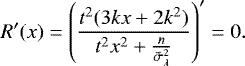
Appendix A Minimising new goodness-of-fit
In Sect. 2.2 we introduced goodness-of-fit Lsed Eq. (7). As in Paper I, by minimisation Lsed we find the optimal values of μd and AK for each model that fit the stellar spectral parameters. Minima can be found as the solution of a system of equations:
 (A.1)
(A.1)
Calculating  and
and  and setting them to zero, we obtain the following system of equations:
 (A.2)
(A.2)
where B = 1 if AK > A0 and B = 0 otherwise. This system is non-linear in μd and has to be solved numerically. As before, we are confident that system Eq. (A.2) has only one solution, because its second equation is linear and because the non-linear first equation has a left side that increases monotonically with μd. The solution of this system gives us the optimal μd and AK for each model, which can be used to produce PDFs of distance modulus and extinction.
Appendix B Method validity analysis
Each model contributes a component, defined by Eq. (7), to the distance modulus PDF. As it was shown in Paper I, without parallaxes these components have exactly the same Gaussian shape, the width of which is defined by the Hessian matrix. When parallaxes are included, this is no longer the case. While  and
and  remain the same, the expression for
  becomes much more complex (see Eq. (9)):
 (B.1)
(B.1)
There are two difficulties arising from Eq. (B.1). Namely, the first summand can be negative, which decreases the value of H0,0 as compared to a case when no parallax is included. This means that an addition of the parallax information can increase the width of the Gaussian contribution of some models to PDFs, broadening the PDFs. The second difficulty is that Eq. (B.1), and therefore the width of the Gaussian contribution of some models to PDFs, now depends, in addition to  , on
, on  and π0, which are constants for a given star, as well as on the parallax value π for a given model. We show that these difficulties can be solved by proving the two following statements:
Statement 1: First summand (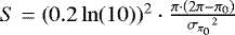 ) of
) of  can be negative, but in this case its contribution will be small, and thus
  is never significantly smaller than
  . The latter sum is the exact value of
  when no parallax information is included.
Statement 2: π can be replaced by π0 in S, as π is close to π0 in all cases where the contribution of S to  is substantial.
B.1 Proof of a Statement 1
The first summand (S) is negative for 0 < π < π0∕2, and reaches its minimum value at π = π0∕4. This minimum value is thus 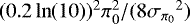 .
.
At the same time, we only consider small values of Lsed, as otherwise the model can be considered to be unreliable. UniDAM produces a solution only if the chi-square probability for the best-fitting model is more than 3%. We require the chi-square probability derived from Lsed for the given model to be at least 0.1% of that for the best model (otherwise its contribution to the PDF will be negligible). This implies that Lsed ≲ 25 if the number of degrees of freedom is 7. The number of degrees of freedom in this case is the number of frequency bands for which visible magnitudes are available plus two – for extinction and parallax.
If we require Lsed < 25, then for π = π0∕2 we get
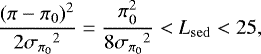 (B.2)
(B.2)
and thus if π < π0∕2 and Lsed < 25, the following should hold:
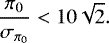 (B.3)
(B.3)
If Eq. (B.3) holds, then the minimum value of S is
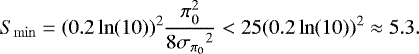 (B.4)
(B.4)
For typical values of  ,
, 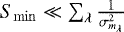 , therefore the contributionof Smin to
  can be neglected.
B.2 Proof of the Statement 2
Here, we want to prove that we can safely replace π with π0 in Eq. (B.1). To do this we want to show that
 (B.5)
(B.5)
or, equivalently, that the fractional error R of  introduced by replacing π with π0 in Eq. (B.1) is
 (B.6)
(B.6)
Let us assume that  , where k should not be very large, so that
 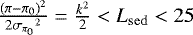 – otherwise Lsed for a given model will be too large for this model to have a non-negligible contribution to PDFs.
Substituting 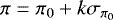 into Eqs. (B.1), we obtain
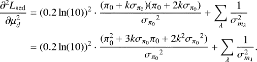 (B.7)
(B.7)
Now, R from Eq. (B.6) will look like:
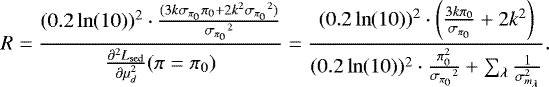 (B.8)
(B.8)
For simplicity, we designate 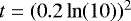 and
and 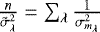 , where n is the number of magnitudes used in Lsed and
  is the average magnitude uncertainty. Using this, we can find the location of the maximum of R as a function of
  by solving the equation:
 (B.9)
(B.9)
Solving this equation for x and substituting to Eq. (B.8), we arrive, after some algebra, to the following expression for the maximum value of R(x):
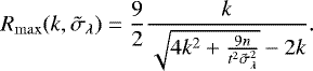 (B.10)
This function indicates the fractional error that we bring into H0,0 by substituting π with π0, as a function of k and average photometric uncertainty  , maximised over all possible
  .
.
The function  is shown for three values of
  (0m. 02 for typical photometry, 0m.05 for bad photometry, and 0m.1 for worst cases) in the top panel of Fig. B.1. The bottom panel of Fig. B.1 shows the same data but now with chi-square probability values
  used as x-axis.
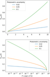 |
Fig. B.1 Fractional error of distance modulus uncertainty, for a single model of a star, as a function of photometric uncertainty and offset k (in units of parallax uncertainty) from the Gaia parallax π0 (top panel) or model probability (bottom panel). |
In UniDAM, we neglect all solutions for which the chi-squared probability of the best model is less than 0.1. In the case when magnitudes in all photometric bands are available, this corresponds to Lsed ≈ 12. Therefore,  and k < 5. For k = 5, we have from Eq. (B.10) that
 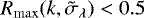 .
.
This means that the error that we bring in by substituting π with π0 in Eq. (B.1) is less than 50%, even for models that have a tiny contribution to the PDFs. Even though this 50% might lead to an incorrectly calculated uncertainty, it is very likely that for cases when both parallax and photometry have high uncertainties, other effects, like the unknown systematics, will be more significant.
Appendix C Additional figures
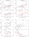 |
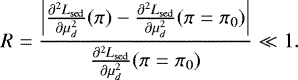
Fig. C.1 As in Fig. 1. We note that for SEGUE survey (subplot j), there are no stars with TGAS parallaxes. |
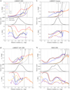 |
Fig. C.1 continued. |
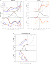 |
Fig. C.1 continued. |
References
- Abolfathi, B., Aguado, D. S., Aguilar, G., et al. 2018, ApJS, 235, 42 [NASA ADS] [CrossRef] [Google Scholar]
- Amôres, E. B., Robin, A. C., & Reylé, C. 2017, A&A, 602, A67 [NASA ADS] [CrossRef] [EDP Sciences] [Google Scholar]
- Astraatmadja, T. L., & Bailer-Jones, C. A. L. 2016, ApJ, 832, 137 [NASA ADS] [CrossRef] [Google Scholar]
- Astropy Collaboration (Robitaille, T. P., et al.) 2013, A&A, 558, A33 [NASA ADS] [CrossRef] [EDP Sciences] [Google Scholar]
- Bressan, A., Marigo, P., Girardi, L., et al. 2012, MNRAS, 427, 127 [NASA ADS] [CrossRef] [Google Scholar]
- Casagrande, L., Schönrich, R., Asplund, M., et al. 2011, A&A, 530, A138 [NASA ADS] [CrossRef] [EDP Sciences] [Google Scholar]
- Casey, A. R., Hawkins, K., Hogg, D. W., et al. 2017, ApJ, 840, 59 [NASA ADS] [CrossRef] [Google Scholar]
- Dalton, G., Trager, S., Abrams, D. C., et al. 2014, Ground-based and Airborne Instrumentation for Astronomy V, Proc. SPIE, 9147, 91470L [Google Scholar]
- de Jong, R. S., Barden, S. C., Bellido-Tirado, O., et al. 2016, Ground-based and Airborne Instrumentation for Astronomy VI, Proc. SPIE, 9908, 99081O [CrossRef] [Google Scholar]
- Gilmore, G., Randich, S., Asplund, M., et al. 2012, The Messenger, 147, 25 [NASA ADS] [Google Scholar]
- Green, G. M., Schlafly, E. F., Finkbeiner, D., et al. 2018, MNRAS, 478, 651 [NASA ADS] [CrossRef] [Google Scholar]
- Ho, A. Y. Q., Ness, M. K., Hogg, D. W., et al. 2017, ApJ, 836, 5 [NASA ADS] [CrossRef] [Google Scholar]
- Hunter, J. D. 2007, Comput. Sci. Eng., 9, 90 [Google Scholar]
- Jones, E., Oliphant, T., Peterson, P., et al. 2001, SciPy: Open Source Scientific Tools for Python [Google Scholar]
- Katz, D., & Brown, A. G. A. 2017, in SF2A-2017, eds. C., Reylé, et al., 259 [Google Scholar]
- Kovalevsky, J. 1998, A&A, 340, L35 [NASA ADS] [Google Scholar]
- Kunder, A., Kordopatis, G., Steinmetz, M., et al. 2017, AJ, 153, 75 [NASA ADS] [CrossRef] [Google Scholar]
- Lindegren, L., Lammers, U., Bastian, U., et al. 2016, A&A, 595, A4 [NASA ADS] [CrossRef] [EDP Sciences] [Google Scholar]
- Luo, A.-L., Zhao, Y.-H., Zhao, G., et al. 2015, Res. Astron. Astrophys., 15, 1095 [NASA ADS] [CrossRef] [Google Scholar]
- Mackereth, J. T., Bovy, J., Schiavon, R. P., et al. 2017, MNRAS, 471, 3057 [NASA ADS] [CrossRef] [Google Scholar]
- Martell, S., Sharma, S., Buder, S., et al. 2017, MNRAS, 465, 3203 [NASA ADS] [CrossRef] [Google Scholar]
- Martig, M., Minchev, I., Ness, M., Fouesneau, M., & Rix, H.-W. 2016, ApJ, 831, 139 [NASA ADS] [CrossRef] [Google Scholar]
- McMillan, P. J., Kordopatis, G., Kunder, A., et al. 2018, MNRAS, 477, 5279 [NASA ADS] [CrossRef] [Google Scholar]
- Michalik, D., Lindegren, L., & Hobbs, D. 2015, A&A, 574, A115 [NASA ADS] [CrossRef] [EDP Sciences] [Google Scholar]
- Mints, A., & Hekker, S. 2017, A&A, 604, A108 [NASA ADS] [CrossRef] [EDP Sciences] [Google Scholar]
- Queiroz, A. B. A., Anders, F., Santiago, B. X., et al. 2018, MNRAS 476, 2556 [NASA ADS] [CrossRef] [Google Scholar]
- Recio-Blanco, A., de Laverny, P., Allende Prieto, C., et al. 2016, A&A, 585, A93 [NASA ADS] [CrossRef] [EDP Sciences] [Google Scholar]
- Schlegel, D. J., Finkbeiner, D. P., & Davis, M. 1998, ApJ, 500, 525 [NASA ADS] [CrossRef] [Google Scholar]
- Sharma, S., Stello, D., Buder, S., et al. 2018, MNRAS, 473, 2004 [NASA ADS] [CrossRef] [Google Scholar]
- Soderblom, D. R. 2010, ARA&A, 48, 581 [NASA ADS] [CrossRef] [Google Scholar]
- Taylor, M. B. 2005, in Astronomical Data Analysis Software and Systems XIV, eds. P. Shopbell, M. Britton, & R. Ebert, ASP Conf. Ser., 347, 29 [Google Scholar]
- Xiang, M., Liu, X., Yuan, H., et al. 2017, MNRAS, 467, 1890 [NASA ADS] [Google Scholar]
- Yanny, B., Rockosi, C., Newberg, H. J., et al. 2009, AJ, 137, 4377 [NASA ADS] [CrossRef] [Google Scholar]
Uploaded to CDS and also available at http://www2.mps.mpg.de/homes/mints/unidam.html
Available at https://github.com/minzastro/unidam
We motivate the use of only infra-red photometry data in Paper I.
All Tables
Ranges of distance modulus μd improvement from the use of Gaia end of mission parallax priors.
Median uncertainties for distance modulus () and log(age) (στ) for five datasets derived for each survey.
Maximum distance modulus μd and a fraction of stars for which the use of parallaxes and spectrophotometric data gives at least 10% improvement in log(age) uncertainties as compared to those obtained with spectrophotometric data alone.
All Figures
|
Fig. 1 Distance modulus uncertainties |
| In the text | |
|
Fig. B.1 Fractional error of distance modulus uncertainty, for a single model of a star, as a function of photometric uncertainty and offset k (in units of parallax uncertainty) from the Gaia parallax π0 (top panel) or model probability (bottom panel). |
| In the text | |
|
Fig. C.1 As in Fig. 1. We note that for SEGUE survey (subplot j), there are no stars with TGAS parallaxes. |
| In the text | |
|
Fig. C.1 continued. |
| In the text | |
|
Fig. C.1 continued. |
| In the text | |
Current usage metrics show cumulative count of Article Views (full-text article views including HTML views, PDF and ePub downloads, according to the available data) and Abstracts Views on Vision4Press platform.
Data correspond to usage on the plateform after 2015. The current usage metrics is available 48-96 hours after online publication and is updated daily on week days.
Initial download of the metrics may take a while.