| Issue |
A&A
Volume 618, October 2018
|
|
|---|---|---|
| Article Number | A62 | |
| Number of page(s) | 14 | |
| Section | Cosmology (including clusters of galaxies) | |
| DOI | https://doi.org/10.1051/0004-6361/201832710 | |
| Published online | 15 October 2018 | |
Iterative map-making with two-level preconditioning for polarized cosmic microwave background data sets
A worked example for ground-based experiments
1
SISSA – International School for Advanced Studies, Via Bonomea 265, 34136 Trieste, Italy
e-mail: This email address is being protected from spambots. You need JavaScript enabled to view it.
, This email address is being protected from spambots. You need JavaScript enabled to view it.
2
Institut d’Astrophysique Spatiale, CNRS (UMR 8617), Univ. Paris-Sud, Université Paris-Saclay, bât. 121, 91405 Orsay, France
3
INFN – National Institute for Nuclear Physics, Via Valerio 2, 34127 Trieste, Italy
4
AstroParticule et Cosmologie, Univ. Paris Diderot, CNRS/IN2P3,CEA/Irfu, Obs de Paris, Sorbonne Paris Cité, France
Received:
26
January
2018
Accepted:
15
May
2018
Abstract
Context. An estimation of the sky signal from streams of time ordered data (TOD) acquired by the cosmic microwave background (CMB) experiments is one of the most important steps in the context of CMB data analysis referred to as the map-making problem. The continuously growing CMB data sets render the CMB map-making problem progressively more challenging in terms of computational cost and memory in particular in the context of ground-based experiments with their operational limitations as well as the presence of contaminants.
Aims. We study a recently proposed, novel class of the Preconditioned Conjugate Gradient (PCG) solvers which invoke two-level preconditioners in the context of the ground-based CMB experiments. We compare them against the PCG solvers commonly used in the map-making context considering their precision and time-to-solution.
Methods. We compare these new methods on realistic, simulated data sets reflecting the characteristics of current and forthcoming CMB ground-based experiments. We develop a divide-and-conquer implementation of the approach where each processor performs a sequential map-making for a subset of the TOD.
Results. We find that considering the map level residuals, the new class of solvers permits us to achieve a tolerance that is better than the standard approach by up to three orders of magnitude, where the residual level often saturates before convergence is reached. This often corresponds to an important improvement in the precision of the recovered power spectra in particular on the largest angular scales. The new method also typically requires fewer iterations to reach a required precision and therefore shorter run times are required for a single map-making solution. However, the construction of an appropriate two-level preconditioner can be as costly as a single standard map-making run. Nevertheless, if the same problem needs to be solved multiple times, for example, as in Monte Carlo simulations, this cost is incurred only once, and the method should be competitive, not only as far as its precision is concerned but also its performance.
Key words: cosmic background radiation / cosmology: observations
© ESO 2018
1. Introduction
Over recent decades, several experiments have looked into the cosmic microwave background (CMB) polarization anisotropies aiming at discovering a stochastic background of gravitational waves produced during the inflationary phase of our Universe encoded in the B-modes, that is, the divergence-free pattern in CMB polarization. Indeed, the amplitude of the CMB B-mode polarization anisotropies at scales larger than 1 degree, conventionally parameterized with a tensor-to-scalar ratio, r, is thought to be directly related to the energy scale of inflation (~1016 GeV). These primordial B-modes have not been detected yet and further progress in both the control of the diffuse polarized emission from our Galaxy (involving widely the microwave frequency regime Ade et al. 2015) and in the sensitivity of the experimental set-ups is necessary in order to reach such a goal. At the sub-degree angular scales, B-modes are produced by the gravitational lensing due to large-scale structures intervening along the photon path travelling towards us. Evidence for these lensing B-modes was first provided via cross-correlation of the CMB polarization maps with the cosmic infrared data (Hanson et al. 2013; The Polarbear Collaboration et al. 2014a) and via constraining the small-scale B-mode power (The Polarbear Collaboration et al. 2014b) and they have since been then characterised with increasing accuracy (Louis et al. 2017; Keisler et al. 2015; BICEP2 Collaboration et al. 2016; The Polarbear Collaboration et al. 2017). While these past experiments have observed the microwave sky with arrays of thousands of detectors often focusing on small sky patches, the forthcoming CMB experiments are planned to observe larger patches with at least tens of thousands of detectors, producing as a result, time-ordered data (TOD) including tens and hundreds of billions of samples.
The recovery of the sky signal from these huge, noisy time streams, a process called map-making, represents one of the most important steps in CMB data analysis and, if the detector noise properties and scanning strategy are known, map-making becomes a linear inverse problem. The generalized least-squares (GLS) equation provides an unbiased solution to map-making for an arbitrary choice of weights given by a symmetric and positive definite matrix (Tegmark 1997a). Moreover, if we consider the inverse covariance of the time domain noise as the weights, the GLS estimate is also a minimum variance and a maximum likelihood solution to the problem. However, computation of the solution in such a case may require either an explicit factorisation of a huge, dense matrix (Tegmark 1997a; Borrill 1999; Stompor et al. 2002) or an application of some iterative procedure (Wright 1996; Oh et al. 1999; Doré et al. 2001; de Gasperis et al. 2005; Cantalupo et al. 2010). These latte typically involve several matrix-vector multiplications at each iteration step. What makes the map-making problem particularly challenging are the sizes of the current and forthcoming CMB data sets which are directly related to the number of floating point operations (flops) needed to achieve the solution and to the memory requirements due to the sizes of the arrays required for it. Both these factors set the requirements on computational resources and indeed many current CMB data analysis pipelines opt for massively parallel computing platforms. However, even in such circumstances, efficient algorithms are necessary to ensure that the analysis can indeed be performed. The computational complexity of the algorithms involving an explicit matrix inversion is  flops, where Np is the number of pixels in the map, and therefore they are only suitable for cases where the estimated sky maps do not involve many sky pixels. Nonetheless, whenever feasible, the direct approaches can yield high-precision, unbiased estimates of the sky signal (e.g. Poletti et al. 2017, for a recent example). The next generations of the ground experiments, CMB-Stage III (Arnold et al. 2014; Henderson et al. 2016; Benson et al. 2014) and IV (Abazajian et al. 2016), however, are expected to observe significant fractions of the entire sky with high resolution, thus resulting in maps with Np ≃ 𝒪(106), rendering the direct approaches prohibitive even for the largest forthcoming supercomputers.
In this context, iterative methods have offered an interesting alternative. They involve algorithms within the class of Krylov methods (e.g. Golub & Van Loan 1996, and references therein), which avoid the explicit inversion of the linear system matrix by constructing an approximate solution which is iteratively improved on. The computational complexity of such methods is mostly driven by matrix-vector products, which need to be performed repeatedly on each iteration. These require at most  flops and can be performed at much lower cost in the specific case of the CMB map-making (see Sect. 3), where such matrix-vector products can be computed matrixfree, that is, without ever explicitly assembling the system matrix in memory (Cantalupo et al. 2010). To date, most of CMB iterative solvers have been based on the Conjugate Gradient (CG) method applied to a preconditioned system of map-making equations and have involved a simple block-diagonal preconditioner (see Eq. (13)). While these solvers usually perform very well (e.g. Ashdown et al. 2009; Cantalupo et al. 2010, and references therein), the anticipated data sets motivate a search for better, more efficient algorithms (Grigori et al. 2012; Naess et al. 2014; Szydlarski et al. 2014; Huffenberger & Næss 2018).
In this paper we apply the methodology proposed by (2014) to a reconstruction of maps from simulated data of a modern, ground-based CMB experiment. This new class of approaches involves constructing and applying a more involved, two-level preconditioner. Our simulations are informed by the experiences derived from the deployment and analysis of the POLARBEAR experiment whose results from the first two seasons of data have recently been published in The Polarbear Collaboration et al. (2017). In Sect. 2.1, we briefly introduce the formalism of the map-making problem in the presence of time domain filtering operators typical for a ground-based CMB experiment. In Sect. 3, we describe the iterative approach and the two different methodologies adopted in the analysis. In Sect. 4 we further describe how the filters introduce degeneracies on the estimation of the maps. The main results of this paper are presented in Sect. 7, where we show a close comparison of the performances of the commonly-used block-diagonal and the two-level preconditioners applied onto realistic simulated data sets. These include signal as well as sky coverage and noise properties representative of the forthcoming generation of CMB polarization experiments. Finally, in Sect. 8 we summarize our main results and conclusions.
2. Map-making in CMB ground-based experiments
2.1. The unbiased estimator
The input data of the map-making procedure are the calibrated TODs collected in a single time domain vector d of size Nt containing all measurements performed during a certain period of time by all the detectors of a CMB experiment. The measurements can be modelled as the sum of an astrophysical signal and measurement noise, nt. The astrophysical contribution to a measurement taken at time t is given by the sky signal, sp, in pixel p observed at time t and which is already convolved with the instrument response, assumed hereafter to be axially symmetric. The correspondence between the sky pixel, p, and the time, t, can be encoded by a sparse and tall (Nt × Np) matrix, Ptp. The data model can then be written as: (1)
(1)
or in the matrix form as, (2)
(2)
Here, s stands for the map to be estimated.
The structure of the pointing matrix encodes the scanning strategy of the CMB experiment and depends on whether the detectors are sensitive or not to the polarization. In the former case, the sky signal is described by three Stokes parameters I, Q, U in every pixel p of the map, that is, sp = (Ip, Qp, Up), and a measurement by a polarization-sensitive experiment taken at time t can be written explicitly as (3)
(3)
where ϕt is the angle of the detector projected onto the sky co-ordinates at time t. In this case, the pointing matrix has three non-zero entries per row. We further assume the noise to have vanishing mean 〈 n 〉 = 0 and to be defined by the noise covariance matrix 𝒩.
Under these assumptions the map-making is a linear inverse problem of estimating the sky signal, s, from the data, d, given the data model as in Eq. (2). This is a linear statistical problem whose solution is provided by a GLS, (4)
(4)
yielding an unbiased estimator (Tegmark 1997b) for any choice of a positive definite matrix W. In particular, if W = 𝒩−1 and the noise is Gaussian distributed, the estimator in Eq. (4) becomes minimum variance.
2.2. The filtering operator
The raw TODs are often contaminated by some unwanted signals that are not astrophysical in their origin, such as the ground pickup or the atmospheric contributions, or their noise properties display strong, long-term correlations commonly referred to as 1/ f noise. All these contributions are usually filtered out from the data.
In such cases, the template of the unwanted signal, T, is known while its amplitude y is not. What a filtering operation is required to do is to remove a component of the TOD contained by the subspace spanned by the columns of T, that is, (5)
(5)
 (6)
(6)
so that d′ · Ti = 0, for any template Ti included as a column of the template matrix, T. The most general form of the filtering operator involves also weighting by a full-rank weight matrix, W, and reads (7)
(7)
With the above definition of FT , it is therefore possible to generalise (4) to Poletti et al. (2017)
 (8)
(8)
We highlight that the filtering operator does not change the properties of the estimator in (8). It is still unbiased,
and if we consider W = 𝒩−1, it is minimum variance.
3. Preconditioned iterative solvers
We can rewrite (8) as a linear system, (9)
(9)
where A is a symmetric and positive definite (SPD) matrix. The CG algorithm is particularly attractive for large sparse or structured systems since it references the system matrix A only through its multiplication of a vector. The convergence rate of the CG depends on the condition number of the system matrix, κ, (Golub & Van Loan 1996), defined as the ratio of the largest to the smallest eigenvalue of a matrix.
To reduce the condition number of A, a preconditioner matrix MP is applied to the linear system so that the condition number of matrix MPA is smaller. If this is the case, the CG converges within a smaller number of iterations. This new algorithm is commonly referred to as preconditioned CG (PCG) as it solves the preconditioned linear system, (10)
(10)
It can be shown (Golub & Van Loan 1996) that the PCG convergence rate is strictly related to the condition number of the pre-conditioned matrix MPA. In fact, after k iterations of the PCG, the magnitude of the error is (11)
(11)
where x is the true solution to (9) and (12)
(12)
is the PCG residual at the kth step.
3.1. The Jacobi preconditioner
From (4) we can define the Jacobi preconditioner: (13)
(13)
This is not only trivial to compute, store, and apply to a vector, but it also accounts for some of the eigenstructure of the actual system matrix, which is due to the inhomogeneity of the sky observations. These properties explain why MBD is the most successful and popular preconditioner used in the current CMB map-making practice. We call it either the block diagonal or Jacobi preconditioner1.
The effect of Jacobi preconditioners on the eigenspectrum of A is to shift the largest eigenvalues towards unity, thus potentially decreasing the condition number of the preconditioned system. However, the nearly singular eigenvalues due to the noise correlations or the filtering will not generally be accounted for. These are common for ground-based experiments and consequently the convergence of the PCG with the block-diagonal preconditioner is often found unsatisfactory. Indeed, in extreme, albeit not uncommon cases, this manifests itself as a saturation of the residuals’ level and a lack of actual convergence down to a required threshold (e.g. Szydlarski et al. 2014).
3.2. Two-level preconditioners
An alternative preconditioner may be found among the class of the so-called Deflation preconditioners that have proven to be successful in the presence of a few isolated extremal eigenvalues. They act as de-projectors from the so-called deflation subspace, 𝒵. This subspace is generated by r linearly independent eigenvectors related to the smallest eigenvalues and constitute the columns of the deflation matrix Z. This matrix is needed to define the projector R (14)
(14)
The projector R is A-orthogonal to any vector w ∈ 𝒵 since RAZ = 0. In the exact precision algebra, R would be a very efficient preconditioner, as for each step of an iterative CG-like solver it would be orthogonal to the null space of the RA. However, we deal with finite precision arithmetic and the zero eigenvalues are often as bothersome as the small ones due to the numerical precision of the machine.
This issue can be solved by combining the operator R with the Jacobi preconditioner, as has been proposed in Szydlarski et al. (2014); (15)
(15)
where E is the coarse operator, defined as E = Z†AZ. M2l is referred to as the two-level preconditioner and we note that it indeed fixes the issue of the zero eigenvalues since they are rescaled all to one. Indeed, (16)
(16)
The dimension of the deflation subspace, given by dim 𝒵 = r, is by construction much smaller than Np, and it is straightforward to invert the matrix E. Moreover, as A is SPD, so is E.
We can summarise the action of the M2l preconditioner, applied on a vector υ, as a projection of the vector υ onto two different subspaces, namely 𝒵 and its orthogonal complement 𝒴. The components of υ are projected onto 𝒵 via the ZE−1Z† term in Eq. (15). In this subspace, the inverse A is very well approximated by M2l, since we have that Eq. (16) holds for any z ∈ 𝒵. On the other hand, M2l acts on a generic vector y ∈ 𝒵 in the same way that MBD does, since
Therefore, once M2l de-projects from the deflation subspace, it performs the PCG by means of the standard preconditioner and it converges faster since MBDA has a smaller condition number 𝒪(10) (due to the considerations made at the end of Sect. 3.1).
It may appear that in order to build the deflation subspace, one would require the knowledge of the entire eigenspectrum of A to determine the eigenvectors with the smallest eigenvalues. However, Szydlarski et al. (2014) have proposed that approximated eigenpairs derived with the help of the so called Ritz approximations (see Appendix A) is sufficient for this purpose.
4. The case of the ground-based experiments
A ground-based CMB experiment, scanning the sky with a focal plane including thousands of polarization-sensitive pixels, has to cope with both atmospheric and ground emissions, which have to be treated on the time domain level. This can be achieved by applying filtering to the data as discussed in Sect. 2.2. The specific templates often applied in this context (e.g. Poletti et al. 2017) are as follows.
In addition to Ritz approximations, it is possible to use Singular Value Decomposition to improve the construction of the deflation subspace. We refer the reader to Pitton & Heltai (2018) for a comparison between several classes of alternative Deflation and Augmentation preconditioners.
4.1. Atmospheric emissions and noise correlations
Both the atmosphere fluctuations, a, and detector noise, n, introduce contributions correlated on long timescales. While such effects could be potentially suppressed by adopting an appropriate weight matrix, W, in practice such a solution is prohibitive given the sizes of the current and anticipated data sets in the time domain. In such cases, the diagonal weight matrices, while straightforward to operate on, will typically lead to poor-quality estimates of the sky signal with strongly correlated, spurious features appearing along the scan directions.
Such long temporal modes can, however, be well approximated by an arbitrary linear combination of piece-wise low-order polynomials. Collecting these templates in a matrix, B, we can express the resulting residual as (17)
(17)
Since Bx is supposed to capture the correlated component of a + n, w is expected to be approximately described by a white noise statistics. Consequently, a diagonal weight matrix can be now sufficient for obtaining good quality sky maps. In our simulations we assume this approximation to be exact and thus simulate TODs with piecewise-stationary white noise.
Filtering these particular modes results in removing long-term trends present in the TODs, whose signal-to-noise ratio is usually very low, from both noise and signal. Even though the stripes in the reconstructed map disappear, we must remember that the constraints on the large angular scales are weak. The system matrix A encodes this information: the presence of the filtering operator (see the left-hand side of Eq. (9)) results in low eigenvalues corresponding to long modes.
4.2. Ground pickup
Though ground-based experiments are designed so that the beam has very low far-side lobes, the signal from the ground is not negligible compared to the CMB one. The elevation is typically constant during an observation period and therefore the ground signal can be considered as a function of the azimuth. If we neglect contributions from other signals, the TOD data model can be written as:
Intuitively, we can think of the second term as the ground template map g projected to the time domain by means of the “ground-pointing matrix” G. This matrix has a column for each azimuthal bin; the entries of the column are equal to 1 whenever the azimuth of the pointing direction falls within the bin range, and are zero elsewhere.
4.3. Map-making for the ground-based experiments
The effects discussed earlier in this section have typical amplitudes that are significantly higher than those of the sky signals, which moreover do not average out efficiently while projected on the sky. For this reason, they need to be treated explicitly in the map-making process by introducing appropriate filters. As elaborated on in Poletti et al. (2017), the required filters, while dealing efficiently with the unwanted contributions, may however render the system matrix, A, ill conditioned, i.e. κ ≫ 1, implying the existence of degeneracies between a certain sky signal s̃ and the amplitude of a certain template ỹ. This means that some particular mode of sky signal is impossible to reconstruct whenever the template ỹ is filtered out, since Ps̃ = Tỹ and P†FPs̃ = P†FTỹ = 0.
This may be particularly acute in the case of the ground pick-up filtering. For a constant-elevation, one-detector observation filtering, ground-stationary signal results in unconstrained modes that are constant in the right-ascension direction.
Accumulating multiple detectors and observation periods can partially break these degeneracies, but the constraints on these modes will typically be weak.
As pointed out earlier, the presence of small eigenvalues in the eigenspectrum of the system matrix, A, can significantly affect the convergence of the iterative solvers and cannot be accounted for by the standard, block-diagonal preconditioner.
5. The simulated data set
In this section, we describe the experimental setup we adopted to perform map-making runs. We exploit the simulation capabilities of the Systematics For CMB (S4CMB) package2 to produce simulated data sets for different experimental configurations of a ground-based experiment located in the Atacama desert in Chile at an altitude of 5190 m. We note that the site location has implications for the properties of the observation. For example, since every pixel is observed at different elevations, the projection of the scan on the sky crosses the pixel in a different direction each time, increasing the so-colled cross-linking (i.e. the coverage in the orientation of the attach angle).
We consider a 60 cm-wide focal plane hosting dual-polarization pixels sensitive to 148 GHz with a fractional bandwidth of 26%. The resolution of the telescope is assumed to be 3.5 arcmin.
We consider three cases that differ for the target sky area and the sensitivity of the instrument, they are summarised in Table 1. The configurations labelled Small Patch (SP) and Large Patch (LP) refer to the characteristics of current and forthcoming CMB experiments observing either small (fsky < 1%) or wide (fsky ≳ 1%) sky patches. For both cases, the noise effective temperature (NET) per detector is  but in LP we increase the number of detectors in the focal plane by about one order of magnitude, from 600 to 8000.
Properties of the different scanning strategies.
We consider an additional case to reproduce a next generation of ground-based CMB experiments that will observe a wider fraction of the sky (fsky ~ 20%) with an increased detector sensitivity  and a larger number of detectors (50 000). We refer to this setup as the Very Large Patch (VLP).
The simulated observations are divided into constant elevation scans (CESs) during which the telescope scans back and forth in azimuth at a speed of 0.4° s−1 and at constant elevation (hereafter, we commonly refer to each azimuthal sweep as a subscan). When the patch has moved out of the field of view, the telescope moves the elevation and azimuth towards the new coordinates of the patch and a new CES starts. The samples are acquired at a rate of 8 Hz, which given our scanning speed is sufficient to reach ℓ ~ 1200. The number of samples per CES depends on the width of the subscan and on the number of detectors performing the measurements.
Using the simulated scanning strategies we scan an input CMB map computed with the synfast routine of the Hierarchical Equal Area Latitute Pixelization (HEALP IX library, Górski et al. 2005)3 and then add a white noise realization corresponding to the sensitivity of each experimental configuration. The input signal power spectrum has been computed with the CAMB package (Lewis et al. 2000) assuming the Planck 2015 best fit cosmological parameters (Planck Collaboration XIII 2016) and r = 0.1. Since we consider maps at a resolution of 3.5 arcmin, we sampled the input CMB signal on a grid with 1.7 arcmin resolution (corresponding to a resolution parameter nside = 2048). The definition of the observed pixels is performed prior to the map-making procedure and is based on discarding those samples that do not observe pixels with enough redundancy.
The simulated TODs acquired by each detector can be expressed as in Eq. (3). However, since the detectors are grouped in pairs sensitive to orthogonal polarization states of the light, commonly referred to as dtop and dbottom, the signal coming from the two detectors of a given pair can be combined in order to disentangle the total intensity and polarization signals without any loss of accuracy by summing and differencing the two signals:
One can, therefore, independently estimate intensity and polarization (expressed via the Q, U Stokes parameters) maps. Two separated data models can be written for the signal and noise component of the time streams: (18)
(18)
 (19)
(19)
where n± is the noise term and can be analogously defined as d± We note that in the following we will neglect possible systematic effects that can leave a residual intensity component in  , such as a calibration mismatch between the two detectors of a pair. The noise properties of the sum and difference time streams are different, as depicted in Fig. 1, and therefore requires a different set of low-order polynomials to be filtered out. In our analysis, the time stream d− is filtered by zeroth and first-order polynomials and d+ is filtered by the first three order polynomials and we assume that these filters completely remove the 1/ f component. For this reason, our noise simulation contains solely white noise. Simulating the correlated noise component is important when evaluating the end-to-end performances of an experiment, but in this paper we focus only on the performances of the map-making solver, which depend mostly on the scanning strategy and data processing adopted. The sum-difference approach and the fact that
  and
and  are uncorrelated allow to separate the intensity and the polarization reconstruction; we take advantage of this by focusing only on the latter for the rest of this paper.
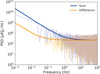 |
Fig. 1. Power spectral density of summing and differencing the signal from simulated data. We highlight the fknee/ f dependence at small frequencies, and the flattening due to white noise above 1 Hz. The solid blue (orange) line refers to a signal with a fknee = 1 (0.05) Hz. |
The ground template is the same for summed and differenced data, and its column number is the same as the number of azicamuthal bins (100 ÷ 1000, depending on the width of the patch). Each azimuth bin has a fixed width of 0.08°. The rows are as many as the number of samples in each 
For simplicity, in the following analysis, we do not build F[G,B]; instead, we avoid the burden of explicit orthogonalization of the filters by using FT in Eq. (9) as the filter, a simplified filter given by FBW−1FGW−1FB, which is explicitly symmetric and would have been equivalent to F[G,B], were the filters FG and FB orthonormal from the outset (Poletti et al. 2017).
6. Constructing two-level preconditoner
A construction of the two-level preconditioner requires knowledge of the deflation operator, 𝒵. We estimate it following the prescription of Szydlarski et al. (2014), which employs the Arnoldi algorithm to compute approximate eigenpairs of the matrix B = MBDA. A suitable selection of these is then used to define the deflation operator, Z. This process has two free parameters, ϵArn and dim 𝒵, which we discuss in the rest of this section and fix in Sect. 7 using numerical experiments.
The Arnoldi algorithm iteratively refines the approximate eigenpairs of the provided matrix and ends the computation when a given tolerance, ϵArn, is reached (see Appendix A for more details). The lower the Arnoldi tolerance, the larger the rank of the approximated B, and, consequently, the larger the number and the accuracy of the estimated eigenpairs. In Fig. 2, the approximated eigenvalues are reported for several choices of ϵArn and some specific choice of the system matrix corresponding to the small patch case is discussed later. It appears that not only the number but also the range of the eigenvalues increase with smaller tolerance. This is intuitively expected since the Arnoldi algorithm relies on the power method (e.g. Golub & Van Loan 1996), and therefore first estimates the largest eigenvalues before moving to the smaller ones. Once the tolerance is as small as 10−9, the range of the estimated eigenvalues starts to saturate. If we attempt to reach a threshold smaller than ~10−12, the Arnoldi iteration proposes a new search direction that, due to the finite numerical precision, has no component linearly independent from the previous ones. Consequently, from that moment on, the algorithm keeps producing eigenvalues equal to zero that are not eigenvalues of B but are simply a sign that the Arnoldi algorithm has converged and exhausted its predictive power. In the studied cases, we find that this typically requires ~150 iterations.
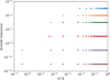 |
Fig. 2. Ritz Eigenvalues MBDA estimated with different Arnoldi algorithm tolerance, ϵArn. A histogram version of this plot can be found in Fig. B.1. |
The computational time required for each Arnoldi iteration is similar to the CG but the memory consumption can be very different: while the Arnoldi needs space for as many vectors as the iteration number, the CG requires only a few vectors in the memory regardless of the iteration number. However, this is not a problem if the size of the map is negligible compared to the time streams – a condition likely to be met in forthcoming ground-based experiments.
The other parameter in the construction of the preconditioner is the dimension of the deflation space. For any given Arnoldi tolerance, this can be either fixed directly by defining the number of the smallest eigenvalue and eigenvectors retained to construct 𝒵 or by defining a threshold below which the eigenvalues and eigenvectors are retained, ϵλ.
7. Results and discussion
In this section, we present the performance comparisons of the standard block-diagonal and the two-level preconditioners both applied on simulated noise or signal-only dataset observing with the scanning strategies listed in Table 1. Moreover, we focus on the reconstruction of the polarization component of the sky, but the results for total intensity are similar and are reported in Appendix B.
7.1. Comparison methodology
We use three types of metric in order to estimate the level of accuracy achievable by each considered approach. First we consider the norm of the standard map-level residuals as defined in Eq. (12) normalized by the norm of the right hand side, i.e. (20)
(20)
This measure of convergence is naturally provided in the CG algorithm and, most importantly, does not require knowledge of the true solution; it is indeed the one typically employed in real applications for measuring the reconstruction quality.
In order to obtain further insight, in this paper we also consider metrics that require knowledge of the exact solution, which is available only in the case of signal-only simulations. We make use of the norm of difference between the true and recovered map defined in Eq. (11), and the bin-by-bin difference between the power spectrum of the input map and reconstructed map, binned using equally spaced bins in multipoles, ℓb, (21)
(21)
with X = E, B; the differences are normalized with respect to the cosmic variance of the input CMB map, (22)
(22)
This power spectrum difference enables us to check which scale in the maps is better constrained, and the normalization gives an estimate of how much the signal intrinsically fluctuates. We stress that we compare against the power spectrum of the input map, not the power spectrum used to simulate it. Therefore, the normalization is simply a reference value and  has no cosmic variance.
As the considered sky patches cover only a fraction of the sky, the power spectra are computed using a pure-pseudo power spectrum estimator X2PURE (Grain et al. 2009). This is a pseudo power spectrum method (Hivon et al. 2002) which corrects the E-to-B-modes leakage arising in presence of incomplete sky coverage (Smith & Zaldarriaga 2007; Bunn et al. 2003; Lewis et al. 2001).
7.2. Setting the two-level preconditioner
We use numerical experiments to show the role of the two free parameters involved in the computation of the two-level pre-conditioner, ϵArn and dim 𝒵. A sample of the results is shown in Fig. 3. In the left panel, we fixed the Arnoldi tolerance to ϵArn = 10−5 and change the dimension of the deflation space from dim 𝒵 = 2–50, which corresponds to varying ϵλ from 0.01 up to 1.
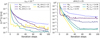 |
Fig. 3. (left) PCG residuals with M2l and MBD preconditioners for several choices of the size of the deflation subspace. Ritz eigenpairs are computed up to a fixed Arnoldi tolerance ϵArn. (right) The M2l is built by selecting a fixed number of Ritz eigenvectors, i.e. dim 𝒵 = 25, computed by running the Arnoldi algorithm with several choices for ϵArn. |
The size of the deflation subspace strongly affects the steepness of the initial convergence. This is expected because if we use all the vectors produced by the Arnoldi algorithm to construct the deflation subspace, the residual after the first iteration is related by construction to the Arnoldi tolerance. On the contrary, the case with the block-diagonal preconditioner corresponds to dim 𝒵 = 0. The more we include vectors in the deflation subspace, the more we approach dim 𝒵 = 50, which retains nearly all the vector produced by the Arnoldi iterations and indeed jumps immediately to a residual close to the Arnoldi tolerance. In our setup, the case with ϵλ = 0.2 (corresponding to dim 𝒵 = 25) delivers a slightly more accurate estimate and will be our value of choice in the rest of this paper. As the threshold of 10−6 is commonly adopted in the CMB map-making procedures for the convergence, these residuals are already quite satisfactory. Moreover, they are also already nearly two orders of magnitude better than what can be achieved with the standard, block-diagonal preconditioner.
We would like to make sure that better precision could be reached if needed. In the right panel of the figure we fix dim 𝒵 to 25 and show how the performances change as the Arnoldi tolerance threshold decreases. The more we decrease the Arnoldi threshold, the lower the value we get for the final residuals – for the reason discussed above, the first few tens of iterations are affected by the fraction of eigenvectors retained rather than ϵArn itself. Choosing ϵArn ~ 10−6 seems already sufficient as it allows us to reach residual levels as low as 10−8; even lower residuals are reached by further decreasing ϵArn. In particular, we did not reach any saturation when we let the Arnoldi converge completely, that is, when ϵArn = 10−14. We might be tempted to always use such a low threshold to build the preconditioner for our CG solver. However, when we push the Arnoldi to a given threshold we are basically solving the system to the same residual threshold with the GMRES algorithm. Therefore, building a two-level preconditioner for a given system using a value of ϵArn much lower than the target CG residual is not meaningful.
We therefore conclude that in order to achieve a very accurate solution (PCG residual tolerance ~10−7 or better) by means of the two-level preconditioner, the Arnoldi algorithm has to converge within a tolerance of ϵArn < 10−6, and dim 𝒵 = 20 ÷ 30 eigenvectors are required to build the deflation subspace.
7.3. Divide-and-conquer map making of one season of observation with a precomputed two-level preconditioner
In the previous section, we have shown that building a two-level preconditioner with a fully converged Arnoldi algorithm gives the best CG convergence rate. Building such a preconditioner may not always be desirable for a single map-making run, given the extra numerical cost. Nonetheless, in this section we show that it typically not only leads to significant performance gains when many similar map-making runs are to be performed, but, in practice, often yields better solutions for some single runs.
We now explore a different scenario, the so-called divide-and-conquer map making, in which we solve for many map-making problems with a system matrix A and right-hand side (RHS) b that are similar but not equal. Cosmic microwave background experiments can only get the best possible map out of their observation if they analyse the whole data set at once.
Nevertheless, splitting the full data volume into smaller groups and producing their maps independently can enormously reduce the computational complexity of map making, since no communication between parallel tasks is needed, permitting one to capitalize on the parallel character of this approach, while still producing high-quality maps.
In the context of the ground-based experiments, which typically scan the same sky area repetitively multiple times, these smaller map-making problems can be defined in such a way that their system matrices A have similar properties.
We explore the performances of the two-level preconditioner in this context starting from simulation of a two-season data set of SP. For this scanning strategy, each CES lasts about 15 min and we split the whole observation into 250 subsets, each consisting of 27 CESs. This subgroup roughly corresponds to all the data taken in a given day. Each processing element performs a PCG run on one such subset, which is characterised by Nt ~ 108 and Np ~ 4 × 10⁴. Given these numbers, we can perform as many as two PCG runs per node of the EDISON computing system4, which provides 64 GB of memory.
We consider different types of two-level preconditioner runs.
-
The “Active” approach: The Ritz eigenpairs are computed for each subset of data. We use dim 𝒵 = 25 (ϵλ = 0.2) but consider two values for ϵArn, 10−6 and 10−12. The former corresponds to the prescription we have given in Sect. 7.2 for the single map-making run. The latter corresponds to the best preconditioner we can have with this technique. We explained earlier that it is not meaningful to build such a preconditioner for a PCG run, but it provides a useful limit case to compare against.
-
The “Simplified” approach: The Ritz eigenpairs are computed only for one subgroup, using dim 𝒵 = 25 and ϵAnr = 10−12. The M2l built from this eigenvector basis is then applied to the rest of the whole data set. This approach is computationally cheaper than the active one, but it is less specific and can work only in the case where the computed deflation basis is very representative of the whole dataset.
Figure 4 reports the histograms of the PCG performances; the left and right panels show the residual at the last iteration and the total number of iterations performed, respectively. The rightmost bin of the latter collects the runs that did not meet the convergence criterion of 10−6 within 100 iterations. This means that, rather than using a preconditioner tailored to the subset of the PCG run, it is important to characterise well the most degenerate modes, even on a slightly different system: the deflation basis computed from a subset of data is very representative of the whole season’s data set. This shows that the simplified approach provides a very effective way of implementing the divide-and-conquer map-making run in the context of the ground-based observations.
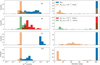 |
Fig. 4. Histograms of (left) residual norms and (right) iteration steps of PCG runs performed on simulated data on SP, LP, and VLP in the top, centre, and bottom panels, respectively. Blue and orange bars show the histogram related to PCG runs with MBD and with M2l applied with the simplified approach, respectively. In the top panel we also show PCG runs applied with the active approach with ϵArn = 10−6 (10−12) as red (green) bars. |
We further test this approach by applying it to observations covering a larger fraction of sky, the LP and VLP scanning strategies. As summarised in Table 1, the noise level in the LP case is about four times lower than the SP one: our aim is to probe the performances of this methodology in terms of the sensitivities achieved in the forthcoming ground-based experiments. For LP, the length of one CES is larger than SP, each one lasting 4 h, and usually we simulate one or two CESs per day, depending on the seasonal availability of the patch above the horizon. We obtain a data set consisting of 350 CESs and we separate this into 50 subgroups, each made of seven CESs. Given the memory size of NERSC computing system CORI (128 GB)5 we can run one of these 50 subgroups per node, meaning that we distribute the seasonal data set across 50 nodes. We construct the twolevel preconditioner by taking one of these subsets and running the Arnoldi iterations up to the numerical convergence, that is, ϵArn = 10−12. We retain the Ritz eigenvectors related to the eigenvalues smaller than 0.2. This yields a deflation subspace with size dim 𝒵 = 28. We then apply the two-level preconditioner to the whole dataset. The comparison of performances between the PCG run with MBD and M2l is shown in Fig. 4, with blue and orange bars, respectively, Even in this case, we adopted the same tolerance, 10−6, and we end the PCG iterations when this tolerance is not achieved within 100 iterations. While most of the MBD runs do not converge, M2l runs converged within a median value of 44 iterations.
The last case to be analysed is the VLP, which targets 20% of the sky with a sensitivity typical of future CMB observatories. Similarly to the SP and LP cases, we compare the performances of the two preconditioners applied to one year of signal-plus-noise observations – a total of 300 simulated 8-h CESs, grouped in 100 subsets of three CESs. We run the map-making solver on 100 processing elements distributed on 100 nodes of the CORI. Consistently with the previous LP case, we apply the M2l with the simplified approach with an Arnoldi tolerance of ϵArn = 10−12. In this case, the deflation subspace is spanned by 15 Ritz eigenvectors. As shown in Fig. 4, also in this case while the MBD rarely converges to the fixed tolerance (10−6), whereas M2l converges within a few tens of iterations.
Further details about the convergence statistics and total computational cost of SP, LP, and VLP can be found in Table 2.
Median, 1σ statistics of residual norms, ||r̂(k) || and computational cost of PCG runs for different scanning strategies.
7.4. Real space convergence
We analyse the convergence performances of the two-level and block-diagonal preconditioners using the norm of the difference as defined in Eq. (11). Compared to the standard PCG residuals, this metric more greatly emphasises the eigenvectors of the system matrix with low eigenvalues. As mentioned earlier this analysis requires knowledge of the exact solution of the system. For this reason, we perform signal-only simulations for a subgroup of all the observational patches discussed in Sect. 7.3 and compare the performance of MBD and M2l, computed with the active approach.
The results, shown in Fig. 5, show that the two-level preconditioner is able to recover the solution with better precision than the one computed with the block-diagonal methodology. The fact that the latter saturates very quickly at a value that is much higher than the PCG residual emphasises further the fact that its convergence is hindered by the nearly degenerate modes, which are down-weighted in the PGC residuals shown in the other plots; for example, Fig. 3. Moreover, the fact that the saturation levels differ case by case in Fig. 5 could be due to the presence of different degeneracies depending on the considered observational patch.
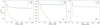 |
Fig. 5. PCG error norms, e(k), as defined in Eq. (11), for a group of 27 signal-only CESs observing SP (left), for a group of 7 signal-only CESs observing LP (centre), and for a group of 3 signal-only CESs observing VLP (right). |
7.5. Convergence at the power spectrum level
We investigate a scale-dependence of the reconstructions by analysing the signal-only study cases considered in the previous section and perform the bin-by-bin power spectra comparison of the residuals as shown in Fig. 6.
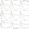 |
Fig. 6. Bin-by-bin comparison of power spectra differences defined in Eq. (21) computed from maps estimated at several iteration steps observing SP (top), LP (centre) and VLP (bottom). We chose different multipole bins to emphasise the convergence behaviour of large, intermediate, and small angular scales. |
For the SP case, the two-level preconditioner converges to the threshold of 10−7 within 40 iterations, whereas for the case with MBD this does not happen within 100 iterations, i.e. the maximum allowed in these runs. We consider the bins that are usually considered in the analysis of patches as small as the SP. As one can see from Fig. 6 (top), the solution computed with MBD encodes an extra bias which is less dominant with respect to the variance of the signal itself by a few percent, meaning that the quality of the map reconstructed with the MBD is acceptable as far as small angular scales are concerned. Moreover, this is somewhat expected since the larger angular scales are not constrained by the MBD and are responsible for the long mode plateau we described in Sect. 4. Those scales are nevertheless unconstrained due to the small sizes of the patch.
LP allows us to probe larger scales, where the primordial gravitational wave B-mode signal is expected to peak. The solution computed with MBD (which does not converge within 100 iterations) shows a ~10% bias at the largest angular scales (i.e. in the first two bins, namely ℓb = 50−100, 150−200 in Fig. 6 (centre panel)), whereas the bias is not present in the solution computed with M2l. This result becomes even more remarkable given that at these scales the signal is likely to be dominated by foreground emission, therefore the same fractional bias in the power-spectrum can be comparable with the whole signal from primordial B-modes. In terms of the norm of the standard residuals, these results demonstrate that high-precision convergence needs to be attained in order to ensure a sufficient precision of the recovered sky signal on all, and specifically on the largest accessible, angular scales.
We observe a similar behaviour with the spectra computed for VLP, Fig. 6 (bottom). In particular, we focus on large scales since the size of the patch is big enough to probe the angular scales related to the reionization peak of both E- and B-modes. We notice that the first two multipole bins, ℓb = 0−50 and ℓb = 50−100, are reconstructed up to percentage level with the two-level preconditioner, whereas the power spectra computed with the block-diagonal one contains a bias which may fluctuate between tens of and a few percent. The degree and subdegree angular scales are similarly reconstructed as in the LP case.
7.6. Monte Carlo simulations
All modern CMB experiments produce or validate their statistical and systematic uncertainties using a large number of simulations. Typically, each of them solves for a map-making system that has the same system matrix A but different RHS b (i.e. the same scanning strategy and data processing but different synthetic time stream). We consider an observation composed of three CESs covering the VLP. We produce 100 Monte Carlo (MC) with not only uncorrelated noise, but even a CMB signal generated using different random seeds from the same CAMB power spectra. We take one of these simulations and build a twolevel preconditioner from a fully converged Arnoldi run. We then apply the same preconditioner to all the simulations. As shown in Fig. 7, all the 100 MC runs converged to a residual tolerance of <10−7 within ~15 iterations and with a staggering narrow dispersion. This result on one hand shows how powerful a two-level preconditioner can be when MC simulations are to be performed, and on the other it shows that the degeneracies preventing the convergence with the standard preconditioner are not due to the signal or the presence of noise, but mostly due to the scanning strategy and the filtering applied to the time stream.
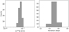 |
Fig. 7. PCG runs performed for 100 MC simulated data points observing the VLP. Notice that all the 100 MC runs converged below a tolerance of 10−7 within ~15 iterations. |
8. Summary and conclusions
In this work, we describe an implementation of a novel class of iterative solvers, the two-level preconditioners, M2l, (Grigori et al. 2012; Szydlarski et al. 2014) in the context of the CMB map-making procedure applied to data sets filtered at the time domain level. We discuss the details of the construction of the new preconditioner and propose a simplified, “divide and conquer” parallel implementation of the method, which can be adequate for an analysis of current and future, ground-based observations. We have tested this new implementation of this novel methodology on three different simulated data sets in the cases when filtering operators typical of the ground experiments, have been applied. We have compared the performance of the method with that of the standard PCG solver based on the Jacobi preconditioner.
We find that in all the studied cases, the two-level preconditioner, M2l, performs better both in terms of the attained precision and the number of required iterations, typically allowing us to reach residuals of the order of 10−7 within 20 ÷ 40 iterations. The standard approach yields residuals an order of magnitude or more higher within as many as 100 iterations. We show that reaching such high precision of the reconstructed maps is required in order to constrain the large angular scales of the B-mode polarization. Indeed, the new approach consistently produces maps typically within 20 ÷ 40 iterations, which display negligible reconstruction bias of all and in particular the longest modes as represented in the maps. On the contrary, the maps derived with the standard solver with the maximal number of iterations set to 100 show typically a 1–20% bias at all scales.
We there conclude that producing highly accurate maps of the polarized CMB anisotropies from the filtered data of the ground-based experiments may call for more advanced iterative solvers than the standard PCG solver with the Jacobi preconditioner. The two-level preconditoner presented here offers significantly better performance and could be a method of choice for such applications in the future. These advantages come, however, at the additional cost needed to construct the preconditioner. Therefore this method could be particularly useful in the cases of large MC simulations, where the additional cost is offset by the solver’s superior performance.
We note that a more typical definition of the Jacobi preconditioner, i.e. diag(A), would not have the same attractive computational properties because its computation would require handling a dense time domain square matrix, 𝒩. The upside of the block diagonal preconditioner is precisely that it takes care of the scanning strategy-induced increase in the condition number without dealing with the complexity of the time domain processing.
Acknowledgments
We acknowledge the use of CAMB, HEALPIX, S4CMB, and X2PURE software packages. We thank Julien Peloton for his help with simulations, and Josquin Errard and Maude Le Jeune for helpful comments and suggestions. RS acknowledges support from the French National Research Agency (ANR) contract ANR-17-C23-0002-01 (project B3DCMB). This research used resources of the National Energy Research Scientific Computing Center (NERSC), a DOE Office of Science User Facility supported by the Office of Science of the U.S. Department of Energy under Contract No. DE-AC02-05CH11231. GF acknowledges the support of the CNES postdoctoral program. CB, DP acknowledge support from the RADIOFOREGROUNDS project, funded by the European Commission’s H2020 Research Infrastructures under the Grant Agreement 687312, and the COSMOS Network from the Italian Space Agency; CB acknowledges support by the INDARK INFN Initiative.
References
- Abazajian, K. N., Adshead, P., Ahmed, Z., et al. 2016, ArXiv e-prints [arXiv:1610.02743] [Google Scholar]
- Ade, P. A. R., Aghanim, N., Ahmed, Z., et al. 2015, Phys. Rev. Lett., 114, 101301 [NASA ADS] [CrossRef] [PubMed] [Google Scholar]
- Arnold, K., Stebor, N., Ade, P. A. R., et al. 2014, in Millimeter, Submillimeter, and Far-Infrared Detectors and Instrumentation for Astronomy VII, Proc. SPIE, 9153, 91531F [NASA ADS] [CrossRef] [Google Scholar]
- Ashdown, M. A. J., Baccigalupi, C., Bartlett, J. G., et al. 2009, A&A, 493, 753 [NASA ADS] [CrossRef] [EDP Sciences] [Google Scholar]
- Benson, B. A., Ade, P. A. R., Ahmed, Z., et al. 2014, in Millimeter, Submillimeter, and Far-Infrared Detectors and Instrumentation for Astronomy VII, Proc. SPIE, 9153, 91531P [NASA ADS] [CrossRef] [Google Scholar]
- BICEP2 Collaboration, Keck Array Collaboration (Ade, P. A. R., et al.) 2016, ApJ, 833, 228 [NASA ADS] [CrossRef] [Google Scholar]
- Borrill, J. 1999, ApJ, ArXiv e-prints [arXiv:astro-ph/9911389] [Google Scholar]
- Bunn, E. F., Zaldarriaga, M., Tegmark, M., & de Oliveira-Costa, A. 2003, Phys. Rev. D, 67, 023501 [NASA ADS] [CrossRef] [Google Scholar]
- Cantalupo, C. M., Borrill, J. D., Jaffe, A. H., Kisner, T. S., & Stompor, R. 2010, ApJS, 187, 212 [NASA ADS] [CrossRef] [Google Scholar]
- de Gasperis, G., Balbi, A., Cabella, P., Natoli, P., & Vittorio, N. 2005, A&A, 436, 1159 [NASA ADS] [CrossRef] [EDP Sciences] [Google Scholar]
- Doré, O., Teyssier, R., Bouchet, F. R., Vibert, D., & Prunet, S. 2001, A&A, 374, 358 [NASA ADS] [CrossRef] [EDP Sciences] [Google Scholar]
- Golub, G. H., & Van Loan, C. F. 1996, Matrix Computations (3rd ed.) (Baltimore, MD, USA: Johns Hopkins University Press) [Google Scholar]
- Górski, K. M., Hivon, E., Banday, A. J., et al. 2005, ApJ, 622, 759 [NASA ADS] [CrossRef] [Google Scholar]
- Grain, J., Tristram, M., & Stompor, R. 2009, Phys. Rev. D, 79, 123515 [Google Scholar]
- Grigori, L., Stompor, R., & Szydlarski, M. 2012, in Proc. International Conference on High Performance Computing, Networking, Storage and Analysis, SC ’12 (Los Alamitos, CA, USA: IEEE Computer Society Press), 91:1 [Google Scholar]
- Hanson, D., Hoover, S., Crites, A., et al. 2013, Phys. Rev. Lett., 111, 141301 [NASA ADS] [CrossRef] [PubMed] [Google Scholar]
- Henderson, S. W., Allison, R., Austermann, J., et al. 2016, J. Low Temp. Phys., 184, 772 [NASA ADS] [CrossRef] [Google Scholar]
- Hivon, E., Górski, K. M., Netterfield, C. B., et al. 2002, ApJ, 567, 2 [NASA ADS] [CrossRef] [Google Scholar]
- Huffenberger, K. M., & Næss, S. K. 2018, ApJ, 852, 92 [NASA ADS] [CrossRef] [Google Scholar]
- Keisler, R., Hoover, S., Harrington, N., et al. 2015, ApJ, 807, 151 [NASA ADS] [CrossRef] [Google Scholar]
- Lewis, A., Challinor, A., & Lasenby, A. 2000, ApJ, 538, 473 [NASA ADS] [CrossRef] [Google Scholar]
- Lewis, A., Challinor, A., & Turok, N. 2001, Phys. Rev. D, 65, 023505 [Google Scholar]
- Louis, T., Grace, E., Hasselfield, M., et al. 2017, JCAP, 6, 031 [NASA ADS] [CrossRef] [Google Scholar]
- Naess, S., Hasselfield, M., McMahon, J., et al. 2014, JCAP, 10, 007 [Google Scholar]
- Oh, S. P., Spergel, D. N., & Hinshaw, G. 1999, ApJ, 510, 551 [NASA ADS] [CrossRef] [Google Scholar]
- Pitton, G., & Heltai, L. 2018, Numerical Linear Algebra with Applications, e2211 https://onlinelibrary.wiley.com/doi/abs/10.1002/nla.2211 [Google Scholar]
- Planck Collaboration XIII. 2016, A&A, 594, A13 [NASA ADS] [CrossRef] [EDP Sciences] [Google Scholar]
- Poletti, D., Fabbian, G., Le Jeune, M., et al. 2017, A&A, 600, A60 [NASA ADS] [CrossRef] [EDP Sciences] [Google Scholar]
- Smith, K. M., & Zaldarriaga, M. 2007, Phys. Rev. D, 76, 043001 [NASA ADS] [CrossRef] [Google Scholar]
- Stompor, R., Balbi, A., Borrill, J. D., et al. 2002, Phys. Rev. D, 65, 022003 [Google Scholar]
- Szydlarski, M., Grigori, L., & Stompor, R. 2014, A&A, 572, A39 [NASA ADS] [CrossRef] [EDP Sciences] [Google Scholar]
- Tegmark, M. 1997a, Phys. Rev. D, 56, 4514 [NASA ADS] [CrossRef] [Google Scholar]
- Tegmark, M. 1997b, ApJ, 480, L87 [NASA ADS] [CrossRef] [Google Scholar]
- The Polarbear Collaboration, (Ade, P. A. R., et al.) 2014a, Phys. Rev. Lett., 112, 131302 [NASA ADS] [CrossRef] [Google Scholar]
- The Polarbear Collaboration, (Ade, P. A. R., et al.) 2014b, ApJ, 794, 171 [NASA ADS] [CrossRef] [Google Scholar]
- The Polarbear Collaboration, (Ade, P. A. R., et al.) 2017, ApJ, 848, 121 [NASA ADS] [CrossRef] [Google Scholar]
- Wright, E. L. 1996, ArXiv e-prints [arXiv:astro-ph/9612006] [Google Scholar]
Appendix A: The Arnoldi algorithm
The Krylov subspace algorithms are based on the construction of a sequence of vectors naturally produced by the power method; a class of those, namely the Minimal Residuals (MINRES) and the Generalized Minimal Residual (GMRES) methods (Golub & Van Loan 1996), rely on the Arnoldi algorithm. Our goal is to find an approximation to the eigenvalues of a matrix B of a generic linear system with RHS b: (A.1)
(A.1)
The Arnoldi algorithm is an algorithm aimed at solving linear systems by projecting the system matrix onto a convenient Krylov subspace generated by the first m vectors (A.2)
(A.2)
The major steps of the algorithm are summarised in Algorithm 1.
Basic steps of the Arnoldi algorithm
Therefore, the output of the Arnoldi algorithm is an orthonormal basis W(m) = (w1|w2|…|wm) (called the Arnoldi vectors), together with a set of scalars hi, j (with i, j = 1, …, m and i ≤ j + 1) plus an extra-coefficient hm+1, m. The former set of coefficient are the elements of an upper Hessenberg matrix Hm with nonnegative subdiagonal elements and is commonly referred to as a m-step Arnoldi Factorization of B. If B is Hermitian, then Hm is symmetric, real, and tridiagonal, and the vectors (columns of W(m)) of the Arnoldi basis are called Lanczos vectors. B and Hm are intimately related via: (A.3)
(A.3)
where em is a 1 × m unit vector with 1 on the mth component.
In other words, Hm is the projection of B onto the subspace generated by the Arnoldi basis W(m) within an error given by  . The iteration loop ends when this error term becomes smaller than a certain threshold ϵArn.
Using Eq. (A.3), we can connect the eigenpairs of B to the ones of Hm. Let us consider an eigenpair of Hm, (λi, yi)
The vector υi = W(m)yi then satisfies (A.4)
(A.4)
The eigenpairs of Hm are therefore approximations of the eigenpairs of B within an error given by W̃m+1. They are the so-called Ritz eigenpairs and are very easy to compute since the size of Hm is ≲ 𝒪(100). For the CMB dataset considered in this work, this is indeed the order of Arnoldi iterations required to reach a tolerance ϵArn ~ 10−6, as can be seen in Fig. A.1. A typical distribution of the amplitude of the Ritz eigenvalues for different values of ϵArn is shown in Fig. B.1.
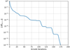 |
Fig. A.1. The convergence residuals of the Arnoldi algorithm. We note that after about 175 iterations, the algorithm numerically converges. |
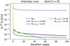 |
Fig. A.2. PCG residuals for SP intensity maps different choices of ϵArn and at a given dim 𝒵 = 25. |
Appendix B: Solving for intensity maps
Similarly to what we have done in Sect. 6, we further tested the two-level preconditioner on SP intensity-only maps. As is shown in Fig. 1, in this case, the time stream has to be filtered with a higher polynomial basis due to a larger fknee. We therefore filter the time streams up to the third-order Legendre polynomials. Figure A.2 shows the PCG residuals for different choices of ϵArn and one can easily notice the similarity to the right panel of Fig. 3. This further indicates that our results are stable even when a more aggressive filter is applied to the data. Moreover, by looking at the blue-dashed line in Fig. A.2, the MBD residuals saturate at a higher threshold with respect to the polarization case (Fig. 3), highlighting the presence of different degeneracies present when intensity maps are involved. However, the twolevel preconditioner does not suffer from this effect and once the Ritz eigenvector basis is very well approximated, by running the Arnoldi algorithm to tolerances below 10−6, it converges to 10−7 within ~ 40 iterations.
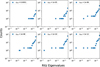 |
Fig. B.1. Histograms of Ritz eigenvalues of the matrix MBDA computed for several choices of Arnoldi tolerance, ϵArn. |
All Tables
Median, 1σ statistics of residual norms, ||r̂(k) || and computational cost of PCG runs for different scanning strategies.
All Figures
|
Fig. 1. Power spectral density of summing and differencing the signal from simulated data. We highlight the fknee/ f dependence at small frequencies, and the flattening due to white noise above 1 Hz. The solid blue (orange) line refers to a signal with a fknee = 1 (0.05) Hz. |
| In the text | |
|
Fig. 2. Ritz Eigenvalues MBDA estimated with different Arnoldi algorithm tolerance, ϵArn. A histogram version of this plot can be found in Fig. B.1. |
| In the text | |
|
Fig. 3. (left) PCG residuals with M2l and MBD preconditioners for several choices of the size of the deflation subspace. Ritz eigenpairs are computed up to a fixed Arnoldi tolerance ϵArn. (right) The M2l is built by selecting a fixed number of Ritz eigenvectors, i.e. dim 𝒵 = 25, computed by running the Arnoldi algorithm with several choices for ϵArn. |
| In the text | |
|
Fig. 4. Histograms of (left) residual norms and (right) iteration steps of PCG runs performed on simulated data on SP, LP, and VLP in the top, centre, and bottom panels, respectively. Blue and orange bars show the histogram related to PCG runs with MBD and with M2l applied with the simplified approach, respectively. In the top panel we also show PCG runs applied with the active approach with ϵArn = 10−6 (10−12) as red (green) bars. |
| In the text | |
|
Fig. 5. PCG error norms, e(k), as defined in Eq. (11), for a group of 27 signal-only CESs observing SP (left), for a group of 7 signal-only CESs observing LP (centre), and for a group of 3 signal-only CESs observing VLP (right). |
| In the text | |
|
Fig. 6. Bin-by-bin comparison of power spectra differences defined in Eq. (21) computed from maps estimated at several iteration steps observing SP (top), LP (centre) and VLP (bottom). We chose different multipole bins to emphasise the convergence behaviour of large, intermediate, and small angular scales. |
| In the text | |
|
Fig. 7. PCG runs performed for 100 MC simulated data points observing the VLP. Notice that all the 100 MC runs converged below a tolerance of 10−7 within ~15 iterations. |
| In the text | |
|
Fig. A.1. The convergence residuals of the Arnoldi algorithm. We note that after about 175 iterations, the algorithm numerically converges. |
| In the text | |
|
Fig. A.2. PCG residuals for SP intensity maps different choices of ϵArn and at a given dim 𝒵 = 25. |
| In the text | |
|
Fig. B.1. Histograms of Ritz eigenvalues of the matrix MBDA computed for several choices of Arnoldi tolerance, ϵArn. |
| In the text | |
Current usage metrics show cumulative count of Article Views (full-text article views including HTML views, PDF and ePub downloads, according to the available data) and Abstracts Views on Vision4Press platform.
Data correspond to usage on the plateform after 2015. The current usage metrics is available 48-96 hours after online publication and is updated daily on week days.
Initial download of the metrics may take a while.