| Issue |
A&A
Volume 618, October 2018
|
|
|---|---|---|
| Article Number | A91 | |
| Number of page(s) | 21 | |
| Section | Catalogs and data | |
| DOI | https://doi.org/10.1051/0004-6361/201731912 | |
| Published online | 15 October 2018 | |
Opening PANDORA’s box: APEX observations of CO in PNe★
1
Leiden Observatory, Leiden University,
Niels Bohrweg 2,
2333 CA
Leiden, The Netherlands
e-mail: This email address is being protected from spambots. You need JavaScript enabled to view it.
2
European Southern Observatory,
Alonso de Córdova 3107,
Santiago, Chile
3
CONACYT Instituto Nacional de Astrofísica, Óptica y Electrónica,
Luis E. Erro 1,
72840
Tonantzintla,
Puebla, Mexico
4
European Southern Observatory,
Karl-Schwarzschild-str. 2,
85748
Garching, Germany
5
Instituto de Astrofísica de Canarias,
38205
La Laguna,
Tenerife, Spain
6
Departamento de Astrofísica, Universidad de La Laguna,
38206
La Laguna,
Tenerife, Spain
7
Department of Physics and Astronomy, University College London,
Gower Street,
London
WC1E 6BT, UK
8
Jodrell Bank Centre for Astrophysics, University of Manchester,
Manchester, UK
9
Department of Physics & Laboratory for Space Research, University of Hong Kong,
Pok Fu Lam Road,
Hong Kong
10
Centre for Research in Earth and Space Sciences, York University,
4700 Keele Street,
Toronto,
ON
M3J 1P3, Canada
11
Joint ALMA Observatory,
Alonso de Córdova 3107,
Vitacura, Santiago, Chile
Received:
7
September
2017
Accepted:
16
March
2018
Abstract
Context. Observations of molecular gas have played a key role in developing the current understanding of the late stages of stellar evolution.
Aims. The survey Planetary nebulae AND their cO Reservoir with APEX (PANDORA) was designed to study the circumstellar shells of evolved stars with the aim to estimate their physical parameters.
Methods. Millimetre carbon monoxide (CO) emission is the most useful probe of the warm molecular component ejected by low- to intermediate-mass stars. CO is the second-most abundant molecule in the Universe, and the millimetre transitions are easily excited, thus making it particularly useful to study the mass, structure, and kinematics of the molecular gas. We present a large survey of the CO (J = 3−2) line using the Atacama Pathfinder EXperiment (APEX) telescope in a sample of 93 proto-planetary nebulae and planetary nebulae.
Results. CO (J = 3−2) was detected in 21 of the 93 objects. Only two objects (IRC+10216 and PN M2-9) had previous CO (J = 3−2) detections, therefore we present the first detection of CO (J = 3−2) in the following 19 objects: Frosty Leo, HD 101584, IRAS 19475+3119, PN M1-11, V* V852 Cen, IC 4406, Hen 2-113, Hen 2-133, PN Fg 3, PN Cn 3-1, PN M2-43, PN M1-63, PN M1-65, BD+30 3639, Hen 2-447, Hen 2-459, PN M3-35, NGC 3132, and NGC 6326.
Conclusions. CO (J = 3−2) was detected in all 4 observed pPNe (100%), 15 of the 75 PNe (20%), one of the 4 wide binaries (25%), and in 1 of the 10 close binaries (10%). Using the CO (J = 3−2) line, we estimated the column density and mass of each source. The H2 column density ranges from 1.7 × 10¹⁸ to 4.2 × 1021 cm−2 and the molecular mass ranges from 2.7 × 10⁻⁴ to 1.7 × 10⁻¹ M⊙.
Key words: line: identification / molecular data / catalogs / (ISM) planetary nebulae: general
The reduced spectra are only available at the CDS via anonymous ftp to cdsarc.u-strasbg.fr (130.79.128.5) or via http://cdsarc.u-strasbg.fr/viz-bin/qcat?J/A+A/618/A91
© ESO 2018
1 Introduction
Planetary nebulae (PNe) represent the final evolutionary phase of low- and intermediate-mass stars, where the extensive mass lost by the star on the asymptotic giant branch (AGB) is ionised by the emerging white dwarf. The ejecta quickly disperses and merges with the surrounding interstellar medium (ISM), whereby the total mass lost from these stars constitutes approximately half of the Milky Way interstellar gas and dust (Leitner & Kravtsov 2011). In the ejecta of AGB stars, the CO molecule locks away the less abundant element, leaving the remaining free oxygen (O) or carbon (C) to drive the chemistry and dust formation. Dust grains and molecules, predominantly CO given the large quantities of C and O in the ejecta, condense in these AGB winds, forming substantial circumstellar envelopes that are detectable in the infrared and millimetre domains. The evolutionary phase between the end of the AGB and the beginning of the planetary nebula (PN) phase has long been a missing link in understanding the late stages of stellar evolution. Observations of molecular gas have played a key role in developing the current understanding of this intermediate phase.
Millimetre and sub-millimetre CO line emission is a very useful probe of the warm molecular component of the neutral gas surrounding AGB stars. This molecule therefore is a standard probe of their envelopes: CO is relatively abundant, and the sub-millimetre transitions are easily excited. In Table 1, we present the general parameters for the most commonly observed CO rotational transitions, including their frequency, density, and their excitation temperature (Eupper/kB). It can therefore be used to study the mass, structure, and kinematics of the bulk of the molecular gas. CO envelopes surrounding PNe have been detected in many CO surveys, including those of Huggins & Healy (1989), using the NRAO 12 m telescope, and Huggins et al. (1996), using the SEST 15 m and IRAM 30 m telescopes. Several recent lines of investigation, including optical imaging of PNe (Sahai & Trauger 1998; López 2003), kinematic studies of proto-planetary nebulae (pPNe; Bujarrabal et al. 2001), and observations of individual molecular envelopes (e.g. He 3-1475 and AFGL 617; Huggins et al. 2004; Cox et al. 2003), have focused the attention on the complex geometry of PN formation. The origins of these complex geometries are not very well understood, but it is very likely that similar structures are found in the molecular gas surrounding young PNe (Huggins et al. 2005) and as such share a formation mechanism.
The dynamical evolution from the AGB to the PN phase has only been observed for a very small sample of objects, which clearly places limits on our understanding of this regime. Knapp et al. (1998) studied CO (J = 2−1) and CO (J = 3−2) in a sample of 45 AGB stars, finding about half of the line profiles to be non-parabolic in shape, with profiles associated with complex winds. Complex line profiles occur when a star is undergoing a change in luminosity, pulsation mode, or chemistry.
Recent improvements in frequency coverage, frequency resolution, and receiver sensitivity enable homogeneous, unbiased, low-noise observationswith high velocity resolution. Motivated by the lack of a large enough sample of observations of PNe in CO, especially the more excited CO (J = 3−2) transition, we observed a sample of 93 young and evolved PNe using the Swedish Heterodyne Facility Instrument (SHeFI) instrument at the Atacama Pathfinder EXperiment (APEX) telescope. We selected the CO (J = 3−2) line rather than lower J transitions because it offers the advantage that higher J transitions have higher critical densities for collisional excitation (see Table 1). For this reason, emission from molecular clouds is less extensive and the observations are less stronglyaffected by contamination of Galactic emission.
We here present the first data release and a preliminary analysis of all the observations. In Sect. 2 we present the observations, Sect. 3 summarises the results, and Sect. 4 presents a discussion of the main outcomes of the survey and future prospects.
Most commonly observed CO transitions with their general parameters.
2 Observations and data reduction
APEX is ideally suited to surveying the CO (J = 3−2) emission from pPNe/PNe in the Southern sky. The atmosphere above Chajnantor has sufficiently transparent conditions (precipitable water vapour, PWV <2.5 mm 80% of the time) to allow CO (J = 3−2) and nearby transitions to be easily detected. The APEX-2 SHeFI receiver with its eXtended bandwidth Fast Fourier Transform Spectrometer (XFFTS) backend, installed at APEX, offers sufficient sensitivity, bandwidth, and spectral resolution to achieve our primary goal of characterising 12CO (J = 3−2) emission in pPNe and PNe. The bandwidth used was 4 GHz, centring the intermediate frequency (IF) at 344.7 GHz.
Data were processed using Continuum and Line Analysis Single-dish Software (CLASS), a part of the GILDAS software1. We subtracted the baselines around the detected CO line to obtain an averaged spectrum of each observation. After this, spectra from all epochs were averaged into a single, final spectrum for each object. To account for the telescope baseline, a polynomial fit of order 3 (in some cases 5) was removed form the averaged spectrum.
APEX observed 93 pPNe and PNe in total. The pPNe sample was extracted from the catalogue of young PNe of Sahai et al. (2011), while the PNe sample was taken from two different sources: PNe that have been observed previously in CO (J = 2−1) by co-author L.-A. Nyman using SEST, and the second from the list of PNe with known binary central stars compiled and maintained by co-author D. Jones2. Targets at |b| < 3.5° were excluded in order to avoid confusion with interstellar CO emission (Dame et al. 2001). Objects with angular dimensions larger than the telescope beam size (18′′) were also excluded (except for IC 4406, NGC 3132, and M2-9). Each source was observed for a total time of 30 min (including overheads), corresponding to a typical on-source time of 6 min, which with nominal Tsys for the expected observing conditions and source elevations (PWV < 2.5 mm) provides a sensitivity of 0.04 K km s−1. The total telescope time dedicated to the survey was 46.5 h.
3 Results
In Table 2 we present the complete list of objects observed, Cols. 1 and 2 are the RA and DEC, respectively, Cols. 3 and 4 contain the PN G and common name of each object, respectively, and Col. 5 shows the rms of the observations for each target in mK. Column 6 specifies whether the line comes from the object or if it is contamination from the interstellar medium (ISM), and Col. 7 refers to the figure in which the final averaged spectrum is shown.
CO (J = 3−2) was detected in 35 of the 93 sources. The spectra of another 7 objects show the CO (J = 3−2) transition inabsorption (negative intensity features); 1 additional object was found to present a line profile with apparent P-Cygni shape. Figures A.1–A.11 show the complete spectrum per object. For the objects with null-detections, the rms value can be used to estimate an upper limit on the CO line intensity.
For the objects where CO (J = 3−2) was detected as a negative intensity feature and for the one object with the apparent P-Cygni shape, the literature velocity of the object was compared with the measured velocity of the line. In all the cases, the negative intensity lines were found to be interstellar CO (J = 3−2) in the OFF positions. The P-Cygni shaped line profile is likely to be caused by emission from a cloud (or two clouds) in both the ON and OFF positions. The line width is also an indication of interstellar material, CO from the ISM has typical line widths of ~1 km s−1 (Hacar et al. 2016), while CO from evolved stars shows line widths of at least a few (up to several tens) km s−1.
Using the same logic, we found that for six objects, the detected CO (J = 3−2) central line velocities do not correspond to the respective velocity of the object and thus are most likely interstellar emission, these were named CO from the ISM. These objects are PN M1-6, IC 4191, PN PC 12, Hen 2-182, PN M3-15, and Hen 2-39.
Therefore we have 21 true CO (J = 3−2) detections. Based on these true detections, we found that CO (J = 3−2) has been detected in two objects, IRC+10216 and PN M2-9 (more detail on their detections is given in the following section). The final number of true CO (J = 3−2) detections that have not previously been reported in the literature is 19. This is the first time that CO (J = 3−2) has been detected in Frosty Leo, HD 101584, IRAS 19475+3119, PN M1-11, V* V852 Cen, IC 4406, Hen 2-113, Hen 2-133, PN Fg 3, PN Cn 3-1, PN M2-43, PN M1-63, PN M1-65, BD+30 3639, Hen 2-447, Hen 2-459, PN M3-35, NGC 3132, and NGC 6326. The following PNe M1-11, Fg 3, Cn3-1, M1-65, Hen 2-133, NGC6326, and M3-35 show line widths smaller than 5 km s−1, therefore these detections should be considered with caution. Each of the detections is discussed in more detail in the following subsections.
In Table 3 we present only the objects with CO (J = 3−2) line detections. Column 1 contains the name of each object, Col. 2 lists the PN G name, Col. 3 the heliocentric velocity in km s−1, Col. 4 presents the line width obtained by the fit in km s−1 (when using several Gaussians, this represents the total width of the line including all components). Column 5 lists the integrated intensity over the velocity range of the line in K km s−1. Columns 6 and 7 show the CO and H2 column density in units of cm−2, Col. 8 refers to the mass estimate of the H2 component in solar masses, and Col. 10 finally refers to the figure where the spectrum is plotted and fitted. All the line intensities were calculated using either a Gaussian fit (for single-peaked lines) or a shell profile fit (for double-peaked lines). In some objects more than one Gaussian line was needed to fit the line profile. Figures 3–5 show the spectra with the detected lines highlighted (the literature values for the heliocentric velocities of the objects are also given). Each line has a fit (either Gaussian or shell) marked in red. Four objects (MPA J1508−6455, Hen 2-447, IRAS 19475+3119, and PN K4-41) have an unknown heliocentric velocity, and it is therefore not indicated in their spectrum.
APEX CO (3–2) observations.
3.1 Proto-planetary nebulae
We detected CO (J = 3−2) in all of the four surveyed pPNe Frosty Leo, IRC+10216, HD 101584, and IRAS 19475+3119. IRC+10216 was known to have CO (J = 3−2) emission, for the other sources this was not the case, and these detections therefore represent the first detections of CO (J = 3−2) in these objects.
APEX CO (J = 3−2) line detections.
Frosty Leo
At first detection of CO (J = 3−2) in this object, its line profile shows much structure, although to first order, it can be fitted with a one-component Gaussian. Previous studies of this object have focussed mainly on CO (J = 2−1) and CO (J = 1−0) (Likkel et al. 1987; Castro-Carrizo et al. 2005; Sahai et al. 2000).
IRC+10216
The CO(J = 3−2) line profile of IRC-10216 was fitted with a one-component Gaussian. IRC+10216 is a very well studied object, the first detection of CO (J = 3−2) in this object was made using the James Clerk Maxwell Telescope (Williams & White 1992). A more detailed study is presented in Patel et al. (2010), where the authors performed a line survey using the Submillimeter Array covering from 293.9 to 354.8 GHz.
HD 101584
At first detection of CO (J = 3−2) in this object, it needed more than one Gaussian to fit the line profile. Many molecular observations of this object can be found in the literature, where CO (J = 2−1) and CO (J = 1−0) have been detected. The first detection of CO (J = 1−0) has been reported by Loup et al. (1990), with further molecular CO studies presented in Trams et al. (1990), Oudmaijer et al. (1995), Olofsson & Nyman (1999), and Olofsson et al. (2015, 2016, 2017).
IRAS 19475+3119
At first detection of CO (J = 3−2) in this object, its line profile can be fitted with a one-component Gaussian. This object has CO (J = 2−1) and CO (J = 1−0) detections in the literature (Likkel et al. 1987; Sánchez Contreras et al. 2006; Sahai et al. 2007; Castro-Carrizo et al. 2010; Hsu & Lee 2011).
3.2 Planetary nebulae
In the sample of 75 PNe, CO (J = 3−2) was detected in 15: in PN M1-11, V* V852 Cen, IC 4406, Hen 2-113, Hen 2-133, PN M2-9, PN Fg 3, PN Cn 3-1, PN M2-43, PN M1-63, PN M1-65, BD+30 3639, Hen 2-447, Hen 2-459, and PN M3-35.
PN M1-11, PN Fg 3, PN Cn 3-1, and PN M1-65
At first dete- ction of CO (J = 3−2) in these objects, the line profiles can be fitted with a one-component Gaussian. No other molecular lines are detected in any of these objects. For all thesesources, the line widths appear to be very narrow. This may indicate that the emission comes from the ISM or might be due to a cloud with the same velocity as the PN. Therefore these detections should be followed-up and confirmed with higher sensitivity instruments).
V* V852Cen
At first detection of CO (J = 3−2) in this object, for its line profile, multiple Gaussian fits were required. This object does not have any other CO lines detected.
IC 4406
At first detection of CO (J = 3−2) in this object, for its line profile, a two-component Gaussian fit was required. The two-component line profile could be associated with an expanding ring, or a disc in rotation. This object has previously been detected in CO (J = 2−1) and CO (J = 1−0) (Cox et al. 1991, 1992; Sahai et al. 1991; Smith et al. 2015).
Hen 2-113
At first detection of CO (J = 3−2) in this object, for its line profile, a three-component Gaussian fit was required. The line profile is very broad; higher resolution might reveal a high-velocity molecular gas component for this object. There are no other CO detections for this object.
Hen 2-133
The heliocentric velocity of PN Hen 2-133 was also unknown, but we found archival observations taken using the Ultraviolet and Visual Echelle Spectrograph (UVES; Dekker et al. 2000) instrument at the Very Large Telescope (VLT; program 095.D-0067(A), PI García-Hernandez). They were reduced using Reflex (Freudling et al. 2013). Emission lines present in the resulting spectrum were fitted using the automated line fitting algorithm (ALFA, Wesson 2016); they indicate a line-of-sight velocity at time of observation of −27.36 km s−1, which was then corrected to heliocentric velocity using the STARLINK RV command (Wallace & Clayton 2014), giving a value of −25.05 km s−1. Using this information, we detect CO (J = 3−2) for the first time in this object. Its line profile can be fitted with a one-component Gaussian. Its line profile is very narrow, which may mean that the line is interstellar rather than nebular, although it shows some broadening at the wings of the line. No other CO lines are detected in this object.
PN M2-9
The CO (J = 3−2) line profile was fitted with a two-component Gaussian. The line shows a beautiful double-peaked profile, which could be interpreted as an indication of a disc or a ring close to the star. The first detection of CO (J = 3−2) in this object was made using the Atacama Large Millimetre/submillimeter Array (ALMA; Castro-Carrizo et al. 2017). CO (J = 2−1) has also been detected in this object using the Plateau de Bure interferometer (Castro-Carrizo et al. 2012).
PN M2-43
At first detection of CO (J = 3−2) in this object, its line profile is very complex. It needed a three-component Gaussian for its fit. This might be an indication of several components, meaning that this object might have much structure, but a further more detailed investigation is needed. CO (J = 3−2) was observed in this object using the JCMT, but only upper limits were obtained (Gussie & Taylor 1995). CO (J = 1−0) was detected in this object using the 13.7 m millimetre-wave telescope of Purple Mountain Observatory (Zhang et al. 2000).
PN M1-63
At first detection of CO (J = 3−2) in this object, its line profile is very complex (similar to M2-9), with a three-component Gaussian needed in order to obtain a reasonable fit. This might be an indication of several components, meaning that this object might have much structure, but a further more detailed investigation is needed. No other CO lines are detected in this object.
BD + 30 3639
This is the first detection of CO (J = 3−2) in this object. The CO (J = 3−2) line profile was fitted using a one-component Gaussian. The molecular observations of CO (J = 2−1) and CO (J = 1−0) in this object were made using the IRAM 30 m telescope (Bachiller et al. 1991), with further molecular CO studies presented in Bachiller et al. (1992), Shupe et al. (1998), Bachiller et al. (2000), and Freeman & Kastner (2016).
Hen 2-447
At first detection of CO (J = 3−2) in this object, its line profile needed a two-Gaussian component for its fit. This might be an indication of a ring or a disc, but a further more detailed investigation is needed. No other CO lines are detected in this object.
Hen 2-459
At first detection of CO (J = 3−2) in this object, its line profile needed only a one-component Gaussian for its fit, although the line is very broad (~100 km s−1). The width of the line might be an indication of a faster component, but a further more detailed investigation is needed. No other CO lines are detected in this object.
PN M3-35
At first detection of CO (J = 3−2) in this object, its line profile needed only a one-component Gaussian for its fit. Its line width is smaller than 5 km s−1, which might be an indication that the emission comes from the ISM rather than the nebula. CO (J = 3−2) was observed in this object using the JCMT, but only upper limits were obtained (Gussie & Taylor 1995).
3.3 Planetary nebulae with binary central stars
Of the initial sample of 93 observed objects, 14 were known to host binary central stars (Jones et al. 2015; Jones & Boffin 2017). Of these 14, 4 are wide binaries (orbital periods ~ 10–1000 days) and 10 are close binaries (orbital periods ~ 1 day). We detected CO (J = 3−2) in emission in only 2 objects: NGC 3132 and NGC 6326.
NGC 3132
The central star of NGC 3132 is a visual binary, and as such is the widest of all the binary central stars observed here (Ciardullo et al. 1999). This is the first time CO (J = 3−2) has been detected in this object. Its line profile is very complex, it needed a three-component Gaussian for its fit. This might be an indication of several components, meaning that this object might have much structure, but a further more detailed investigation is needed. This object was previously observed with the 12 m National Radioastronomy Observatory (NRAO) antenna at Kitt Peak, but CO (J = 3−2) was not detected (Phillips et al. 1992). Further molecular CO (J = 2−1) and CO (J = 1−0) studies on this object are presented in Zuckerman et al. (1990) and Sahai et al. (1990).
NGC 6326
The central star of NGC 6326 close binary system with a period less than one day (Miszalski et al. 2011). NGC 6326 shows CO (J = 3−2). This is the first time CO (J = 3−2) has been detected in this object. The line width is smaller than 4 km s−1, which mightbe an indication that the emission comes from the ISM rather than the nebula. The line profile could be fitted with a one-component Gaussian.
3.4 Sources where the line velocity does not match the PN velocity
The following PNe show CO (J = 3−2) emission lines, but the line is either at a different velocity than the object (therefore might not be associated to the object) or the line is too thin (and therefore associated to interstellar CO (J = 3−2). For IC 4191, PN PC 12, PN M3-15, and Hen 2-39 these CO (J = 3−2) seems to be more likely to be emission form the ISM.
PN M1-6
At first detection of CO (J = 3−2) in this object, its line profile can be fitted with a one-component Gaussian. CO (J = 3−2) emission is detected at around 15 km s−1, while the heliocentric velocity of this object is reported to be 65.5 km s−1 (see references in the table).
IC 4191
At first detection of CO (J = 3−2) in this object, its line profile can be fitted with a one-component Gaussian. CO (J = 3−2) emission is detected at around 10 km s−1, while the heliocentric velocity of this object is reported to be −18.3 km s−1 (see references in the table). Since the line profile of this object is very thin, this emission is likely associated with the ISM. No other molecular lines are detected in this object.
PN PC 12
At first detection of CO (J = 3−2) in this object, its line profile can be fitted with a one-component Gaussian. CO (J = 3−2) emission is detected at around 8 km s−1, while the heliocentric velocity of this object is reported to be −60.3 km s−1 (see references in the table). Since the line profile of this object is very thin, this emission is likely associated with the ISM. No other CO lines are detected in this object.
Hen 2-182
At first detection of CO (J = 3−2) in this object, its line profile can be fitted with a one-component Gaussian. CO (J = 3−2) emission is detected at around 10km s−1, while the heliocentric velocity of this object is reported to be −89.5 km s−1 (see references in the table). The line profile does not seem as narrow as the lines associated with emission from the ISM, but further confirmation is required. No other CO lines are detected in this object.
PN M3-15
At first detection of CO (J = 3−2) in this object, its line profile can be fitted with a one-component Gaussian. The CO (J = 3−2) emission presents at around 10 km s−1, while the heliocentric velocity of this object is reported to be 97.2 km s−1 (see references in the table). Since the line profile of this object is very thin, this emission is likely to originate from the ISM. No other CO lines are detected in this object.
Hen 2-39
The central star of Hen 2-39 is a barium star, and as such, is a wide binary system (although the exact orbital period is unknown; Miszalski et al. 2013). This is the first time CO (J = 3−2) has been detected in this object. Its line profile can be fitted with a one-component Gaussian. The line profile on this object is very thin, and even though it is centred at the nebular heliocentric velocity, this line could still be associated with emission from the ISM. Further investigation is needed. No other CO lines are detected in this object.
3.5 Column density and masses
We estimated the column density N(CO) and N(H2) for all the sources with CO (J = 3−2) detections (see Table 3). Using N(H2), we estimated the molecular mass of each source.
The column density calculations assume optically thin emission and local thermal equilibrium (LTE). Under these assumptions, the CO column density, N(CO), is proportional to the line integrated intensity. We followed the standard formulations to obtain CO column densities (e.g. Huggins et al. 1996), assuming an excitation temperature of 15 K for all objects. Hence the correlation between N(CO) and the CO (J = 3−2) integrated intensity is given by N(CO) = 6.59 × 10¹⁴ ×∫ CO (J = 3−2) dv. The N(CO) values reported in Table 3 include the beam filling factor corrections estimated using the source sizes reported in Table 4. The molecular hydrogen column density, N(H2), is then obtained multiplying N(CO) by the abundance ratio X (CO/H2=) 3 × 10⁻⁴ (see, e.g. Huggins et al. 1996). Finally, to compute the H2 mass, spherical symmetry is assumed and the distances to nebulae listed in Table 4.
We assumed the CO emission of the nebula to be distributed in a uniform sphere and did not take CO photodissociation into account, therefore nebula masses presented here should be taken with a degree of caution. We also assumed optically thin line emission, which means that for those nebulae where this assumption does not hold, the mass estimates should be taken as lower limits.
The NH2 values range from 1.7 × 10¹⁸ to 4.2 × 1021 cm−2. The molecular masses have values in the range from 2.7 × 10⁻⁴ to 1.7 × 10⁻¹ M⊙, which is in the same range as was found by Huggins et al. (1996).
Following Huggins et al. (1996), we plot the masses vs. the distance to each source. In Fig. 1 we present the distribution of masses estimated with respect to their distance. Black squares are the objects from this paper, and for comparison, we also plot the values taken from Huggins et al. (1996), which are represented here as the blue dots. This figure shows that the mass is spread over almost four orders of magnitude, and a correlation between mass and distance is expected, meaning that observationally, we are biased to see the most massive objects at greater distance.
It is difficult to draw strong conclusions from the mass estimates because of the significant assumptions them. However, the mass estimates of these nebulae calculated using the CO made whilst calculating (J = 3−2) transition are very similar to those determined using CO (J = 2−1) or CO (J = 1−0), indicating that these transitions trace similar regions of the nebula. It might have been expected that the CO (J = 3−2) would trace a hotter inner region of the nebula (torus/disc), but this seems to not be the case.
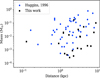 |
Fig. 1 Distance to the source vs. the molecular mass of its envelope. The plot combines the data from this work (black squares) with the data published by (Huggins et al. 1996; blue dots). |
RADEX diagnostic plot
We used the offline version of RADEX (van der Tak et al. 2007) to generate a diagnostic plot for the CO (J = 3−2) to CO (J = 2−1) intensity ratio as a function of kinetic temperatures and H2 volume densities for the sources that had complementary CO (J = 2−1) observations. Only a few sources are reported in the literature with the appropriate data to analyse them together with our CO (J = 3−2) observations. BD+30 3639 was the source with the best complementary CO (J = 2−1) data, given the size of the source and the beam size of the CO (J = 2−1) observations. A discussion of the use of these diagnostic plots is presented for different molecules in the Appendix of van der Tak et al. (2007). Linear molecules, such as CO, are density probes at low densities, while at higher densities, the line ratios are more sensitive to temperature. However, with no other information than a single line ratio (such as our case), it is only possible to provide lower limits to density and temperature.
In Fig. 2 we show the diagnostic plot for the CO (J = 3−2) to CO (J = 2−1) intensity ratio, assuming 2.73 K as the background temperature and a line width of 50 km s−1. The plot shows the results for a column density of 1 × 1016 cm−2, but we find that the CO line ratio is not very sensitive to column density within the range 3 × 1015 cm−2 to ~4 × 1016 cm−2. The plotted ratios corresponded to the observed values for BD+30 3639 (1.6), NGC 3132 (1.3), IC 4406, and M2-9 (0.7, for the last two). However, for the latter three sources, the measured ratios are only lower limits because of different CO (J = 2−1) and CO (J = 3−2) beam sizes (the former larger than the latter) and the source size (larger than both beam sizes). The CO intensity ratio constrains a lower limit to the H2 volume density, nH2 > 103–103.7 cm−3, and kinetic temperature, Tkin > 10–35 K. The highest lower limit values are given for IC 4406 and M2-9.
Size, distance, and morphology of PNe with CO emission.
3.6 Correlation with H2
We would like to probe the relationship between the detection of CO and H2. We compared our sample with the sample analysed by Kastner et al. (1996), whose study was made by imaging the molecular hydrogen emission (λ = 2.122 μm) using the near-infrared cryogenic optical bench mounted at Kitt Peak National Observatory, from the National Optical Astronomy Observatories. They observed 60 PNe and detected H2 in 23 of them. When compared with out sample, 9 objects are in common. Of these 9 objects, 4 were detected in H2, and all are also detected in CO as part of our survey. The objects are NGC 3132, IC 4406, PN M2-9, and BD+30 3639. The remaining objects (five) were not detected in H2 and are they detected here in CO either. These PNe are PN M3-2, PN MyCn18, NGC 6778, NGC 6790, and HD 193538. Although the overlap between PANDORA and the H2 survey of Kastner et al. (1996) is small, we find a clear correlation between the detection of CO and the detection of H2.
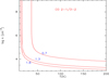 |
Fig. 2 Results from the LVG analysis of the CO lines. The curves represent the predicted CO (J = 3−2) to CO (J = 2–1) intensity ratio for a column density of 1 × 1016 cm−2 and line width of 50 km s−1. The ratios that match the observed CO line ratio and are indicated with solid red curves. |
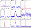 |
Fig. 3 APEX CO (3–2) line detections in pPNe and PNe. |
3.7 Morphology
We investigated the morphological classification for the all the PNe that were observed. The morphology of the sources is included in Tables 2 and 4 for reference. Table 2 lists all the sources, whilst Table 4 lists only those with CO detections. The different morphologies are B (bipolar), E (elliptical), R (round), I (irregular), and S (symmetric) according to the Hong Kong/AAO/Strasbourg Hα planetary nebula database (HASH; Bojicic et al. 2017). The HASH planetary nebula database is an online research platform providing free and easy access to the largest and most comprehensive catalogue of known Galactic PNe and a repository of observational data (imaging and spectroscopy) for these and related astronomical objects. The number of sources with the same morphology are 6 with no morphology, 12 S (symmetric), 7 R (round), 1 I (irregular), 26 E (elliptical), and 41 B (bipolar).
We find that CO (J = 3−2) was detected in the 6 sources that have no morphology classification, in 9 out of the 26 ellipticals, and 9 out of the 41 PNe with bipolar morphology. CO (J = 3−2) was not detected in any of the symmetric, round, or irregular PNe. This bipolar fraction amongst the PNe with CO emission is a lower limit, since the ellipticals could also be bipolar, depending on the viewing angle (Jones et al. 2012). We can conclude that CO (J = 3−2) is more likely to be found in PNe with bipolar or elliptical morphologies than in symmetric, round, or irregular PNe.
4 Conclusions
We present the largest survey of the CO (J = 3−2) line ever taken using the Atacama Pathfinder EXperiment (APEX) telescope in a sample of 93 pPNe and PNe. This survey was designed to study the circumstellar shells of evolved stars with the aim to investigate their physical parameters. Of the 93 objects, we detected CO (J = 3−2) in 35, and another 14 observations show spurious detections associated with the ISM.
CO (J = 3−2) has been detected in two objects, IRC+10216 and PN M2-9. The final number of true CO (J = 3−2) first detections is 19; 3 pPNe and 16 PNe (including one known to host wide binaries and one known to host a close binary central star).
Evaluating the success rates of detection for different object types within our sample, CO (J = 3−2) was detected in all 4 pPNe (100% success rate), 15 of the 74 PNe (20% success rate), one of the 4 wide binaries (25% success rate), and 1 of the 10 close binaries (10% success rate).
Using the CO (J = 3−2) line, we estimated the column density and mass of each source. The H2 column density ranges from 1.7 × 10¹⁸ to 4.2 × 1021 cm−2, and the molecular mass ranges from 2.7 × 10⁻⁴ to 1.7 × 10⁻¹ M⊙
Although the overlap between PANDORA and the H2 survey of Kastner et al. (1996) is small, we find a clear correlation between the detection of CO and the detection of H2, all the sources that show H2 also present CO (J = 3−2) and also vice versa all the sources that do not present H2 also do not present CO (J = 3−2).
An interesting and perhaps somewhat unexpected correlation was found with morphology in that CO (J = 3−2) will be preferentially found in PN with bipolar or elliptical morphologies (the uncertainty in the final fraction is due to the ambiguity of morphology with viewing angle).
Data from the literature, CO (J = 2−1) for three sources and the RADEX software were used to constrain a lower limit to the H2 volume density, nH2 > 103 –103.7 cm−3, and kinetic temperature, Tkin > 10–35 K.
The results presented here represent an extremely valuable catalogue for use in selecting the samples for future follow-up observationswith the Atacama Large Millimetre and sub-millimetre Array (ALMA), particularly in sampling the spatial distribution of the molecular gas in these objects.
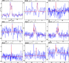 |
Fig. 4 APEX CO (3–2) line detections in pPNe and PNe. |
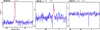 |
Fig. 5 APEX CO (3–2) line detections in pPNe and PNe. |
Acknowledgements
We all thank the anonymous referee for all the comments and suggestions. LGR thanks the time allocation committee for all the telescope time awarded at APEX(SHeFI). LGR is co-funded under the Marie Curie Actions of the European Commission(FP7-COFUND). RW is supported by European Research Grant SNDUST. DJ acknowledges the support by the Spanish Ministry of Economy and Competitiveness (MINECO) under the grant AYA2017-83383-P.
Appendix A APEX full spectrum of each source
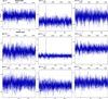 |
Fig. A.1 pPNe and PNe observations using the APEX telescope. |
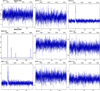 |
Fig. A.2 pPNe and PNe observations using the APEX telescope. |
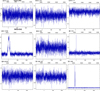 |
Fig. A.3 pPNe and PNe observations using the APEX telescope. |
 |
Fig. A.4 pPNe and PNe observations using the APEX telescope. |
 |
Fig. A.5 pPNe and PNe observations using the APEX telescope. |
 |
Fig. A.6 pPNe and PNe observations using the APEX telescope. |
 |
Fig. A.7 pPNe and PNe observations using the APEX telescope. |
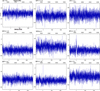 |
Fig. A.8 pPNe and PNe observations using the APEX telescope. |
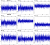 |
Fig. A.9 pPNe and PNe observations using the APEX telescope. |
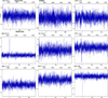 |
Fig. A.10 pPNe and PNe observations using the APEX telescope. |
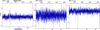 |
Fig. A.11 pPNe and PNe observations using the APEX telescope. |
References
- Acker, A., Cuisinier, F., Stenholm, B., & Terzan, A. 1992, A&A, 264, 217 [NASA ADS] [Google Scholar]
- Bachiller, R., Huggins, P. J., Cox, P., & Forveille, T. 1991, A&A, 247, 525 [NASA ADS] [Google Scholar]
- Bachiller, R., Huggins, P. J., Martin-Pintado, J., & Cox, P. 1992, A&A, 256, 231 [NASA ADS] [Google Scholar]
- Bachiller, R., Forveille, T., Huggins, P. J., Cox, P., & Maillard, J. P. 2000, A&A, 353, L5 [NASA ADS] [Google Scholar]
- Bojicic, I. S., Parker, Q. A., & Frew, D. J. 2017, IAU Symp., 323, 327 [NASA ADS] [Google Scholar]
- Bujarrabal, V., Castro-Carrizo, A., Alcolea, J., & Sánchez Contreras, C. 2001, A&A, 377, 868 [NASA ADS] [CrossRef] [EDP Sciences] [Google Scholar]
- Cahn, J. H., Kaler, J. B., & Stanghellini, L. 1992, A&AS, 94, 399 [NASA ADS] [Google Scholar]
- Castro-Carrizo, A., Bujarrabal, V., Sánchez Contreras, C., Sahai, R., & Alcolea, J. 2005, A&A, 431, 979 [NASA ADS] [CrossRef] [EDP Sciences] [Google Scholar]
- Castro-Carrizo, A., Quintana-Lacaci, G., Neri, R., et al. 2010, A&A, 523, A59 [NASA ADS] [CrossRef] [EDP Sciences] [Google Scholar]
- Castro-Carrizo, A., Neri, R., Bujarrabal, V., et al. 2012, A&A, 545, A1 [NASA ADS] [CrossRef] [EDP Sciences] [Google Scholar]
- Castro-Carrizo, A., Bujarrabal, V., Neri, R., et al. 2017, A&A, 600, A4 [NASA ADS] [CrossRef] [EDP Sciences] [Google Scholar]
- Ciardullo, R., Bond, H. E., Sipior, M. S., et al. 1999, AJ, 118, 488 [NASA ADS] [CrossRef] [Google Scholar]
- Cox, P., Huggins, P. J., Bachiller, R., & Forveille, T. 1991, A&A, 250, 533 [NASA ADS] [Google Scholar]
- Cox, P., Omont, A., Huggins, P. J., Bachiller, R., & Forveille, T. 1992, A&A, 266, 420 [NASA ADS] [Google Scholar]
- Cox, P., Huggins, P. J., Maillard, J.-P., et al. 2003, ApJ, 586, L87 [NASA ADS] [CrossRef] [Google Scholar]
- Dame, T. M., Hartmann, D., & Thaddeus, P. 2001, ApJ, 547, 792 [NASA ADS] [CrossRef] [Google Scholar]
- Dekker, H., D’Odorico, S., Kaufer, A., Delabre, B., & Kotzlowski, H. 2000, in Optical and IR Telescope Instrumentation and Detectors, eds. M. Iye, & A. F. Moorwood, Proc. SPIE, 4008, 534 [Google Scholar]
- Dougados, C., Rouan, D., & Lena, P. 1992, A&A, 253, 464 [NASA ADS] [Google Scholar]
- Durand, S., Acker, A., & Zijlstra, A. 1998, A&AS, 132, 13 [NASA ADS] [CrossRef] [EDP Sciences] [Google Scholar]
- Freeman, M. J., & Kastner, J. H. 2016, ApJS, 226, 15 [NASA ADS] [CrossRef] [Google Scholar]
- Freudling, W., Romaniello, M., Bramich, D. M., et al. 2013, A&A, 559, A96 [NASA ADS] [CrossRef] [EDP Sciences] [Google Scholar]
- Frew, D. J. 2008, PhD Thesis, Department of Physics, Macquarie University, NSW 2109, Australia [Google Scholar]
- Groenewegen, M. A. T., Barlow, M. J., Blommaert, J. A. D. L., et al. 2012, A&A, 543, L8 [NASA ADS] [CrossRef] [EDP Sciences] [Google Scholar]
- Gussie, G. T., & Taylor, A. R. 1995, MNRAS, 273, 801 [NASA ADS] [CrossRef] [Google Scholar]
- Guzmán, L., Gómez, Y., & Rodríguez, L. F. 2006, Rev. Mexicana Astron. Astrofis., 42, 127 [NASA ADS] [Google Scholar]
- Hacar, A., Alves, J., Burkert, A., & Goldsmith, P. 2016, A&A, 591, A104 [NASA ADS] [CrossRef] [EDP Sciences] [Google Scholar]
- Hsu, M.-C., & Lee, C.-F. 2011, ApJ, 736, 30 [NASA ADS] [CrossRef] [Google Scholar]
- Huggins, P. J., & Healy, A. P. 1989, ApJ, 346, 201 [NASA ADS] [CrossRef] [Google Scholar]
- Huggins, P. J., Bachiller, R., Cox, P., & Forveille, T. 1996, A&A, 315, 284 [NASA ADS] [Google Scholar]
- Huggins, P. J., Muthu, C., Bachiller, R., Forveille, T., & Cox, P. 2004, A&A, 414, 581 [NASA ADS] [CrossRef] [EDP Sciences] [Google Scholar]
- Huggins, P. J., Bachiller, R., Planesas, P., Forveille, T., & Cox, P. 2005, ApJS, 160, 272 [NASA ADS] [CrossRef] [Google Scholar]
- Jones, D., & Boffin, H. M. J. 2017, Nat. Astron., 1, 0117 [CrossRef] [Google Scholar]
- Jones, D., Mitchell, D. L., Lloyd, M., et al. 2012, MNRAS, 420, 2271 [NASA ADS] [CrossRef] [Google Scholar]
- Jones, D., Boffin, H. M. J., Rodríguez-Gil, P., et al. 2015, A&A, 580, A19 [NASA ADS] [CrossRef] [EDP Sciences] [Google Scholar]
- Kastner, J. H., Weintraub, D. A., Gatley, I., Merrill, K. M., & Probst, R. G. 1996, ApJ, 462, 777 [NASA ADS] [CrossRef] [Google Scholar]
- Kharchenko, N. V., Scholz, R.-D., Piskunov, A. E., Röser, S., & Schilbach, E. 2007, Astron. Nachr., 328, 889 [NASA ADS] [CrossRef] [Google Scholar]
- Knapp, G. R., Young, K., Lee, E., & Jorissen, A. 1998, ApJS, 117, 209 [NASA ADS] [CrossRef] [Google Scholar]
- Leitner, S. N.,& Kravtsov, A. V. 2011, ApJ, 734, 48 [NASA ADS] [CrossRef] [Google Scholar]
- Likkel, L., Morris, M., Omont, A., & Forveille, T. 1987, A&A, 173, L11 [NASA ADS] [Google Scholar]
- López, J. A. 2003, in Planetary Nebulae: Their Evolution and Role in the Universe, eds. S. Kwok, M. Dopita, & R. Sutherland, IAU Symp., 209, 483 [NASA ADS] [Google Scholar]
- Loup, C., Forveille, T., Omont, A., & Nyman, L. A. 1990, A&A, 227, L29 [NASA ADS] [Google Scholar]
- Miszalski, B., Jones, D., Rodríguez-Gil, P., et al. 2011, A&A, 531, A158 [NASA ADS] [CrossRef] [EDP Sciences] [Google Scholar]
- Miszalski, B., Boffin, H. M. J., Jones, D., et al. 2013, MNRAS, 436, 3068 [NASA ADS] [CrossRef] [Google Scholar]
- Olofsson, H., & Nyman, L.-Å. 1999, A&A, 347, 194 [NASA ADS] [Google Scholar]
- Olofsson, H., Vlemmings, W. H. T., Maercker, M., et al. 2015, A&A, 576, L15 [NASA ADS] [CrossRef] [EDP Sciences] [Google Scholar]
- Olofsson, H., Vlemmings, W. H. T., Maercker, M., et al. 2016, J. Phys. Conf. Ser., 728, 042005 [CrossRef] [Google Scholar]
- Olofsson, H., Vlemmings, W. H. T., Bergman, P., et al. 2017, A&A, 603, L2 [NASA ADS] [CrossRef] [EDP Sciences] [Google Scholar]
- Oudmaijer, R. D., Waters, L. B. F. M., van der Veen, W. E. C. J., & Geballe, T. R. 1995, A&A, 299, 69 [NASA ADS] [Google Scholar]
- Patel, N. A., Young, K. H., Wilson, R. W., et al. 2010, in AAS Meeting Abstracts #215, Bull. Am. Astron. Soc., 42, 541 [NASA ADS] [Google Scholar]
- Phillips, J. P., Williams, P. G., Mampaso, A., & Ukita, N. 1992, Ap&SS, 188, 171 [NASA ADS] [CrossRef] [Google Scholar]
- Quintana-Lacaci, G., Cernicharo, J., Agundez, M., et al. 2016, ApJ, 818, 192 [NASA ADS] [CrossRef] [Google Scholar]
- Robinson, G., Smith, R. G., & Hyland, A. R. 1992, MNRAS, 256, 437 [NASA ADS] [CrossRef] [Google Scholar]
- Sahai, R., & Trauger, J. T. 1998, AJ, 116, 1357 [NASA ADS] [CrossRef] [Google Scholar]
- Sahai, R., Wootten, A., & Clegg, R. E. S. 1990, A&A, 234, L1 [NASA ADS] [Google Scholar]
- Sahai, R., Wootten, A., Schwarz, H. E., & Clegg, R. E. S. 1991, A&A, 251, 560 [NASA ADS] [Google Scholar]
- Sahai, R., Bujarrabal, V., Castro-Carrizo, A., & Zijlstra, A. 2000, A&A, 360, L9 [NASA ADS] [Google Scholar]
- Sahai, R., Sánchez Contreras, C., Morris, M., & Claussen, M. 2007, ApJ, 658, 410 [NASA ADS] [CrossRef] [Google Scholar]
- Sahai, R., Morris, M. R., & Villar, G. G. 2011, AJ, 141, 134 [NASA ADS] [CrossRef] [Google Scholar]
- Sánchez Contreras, C., Bujarrabal, V., Castro-Carrizo, A., Alcolea, J., & Sargent, A. 2006, ApJ, 643, 945 [NASA ADS] [CrossRef] [Google Scholar]
- Santander-García, M., Corradi, R. L. M., Mampaso, A., et al. 2008, A&A, 485, 117 [NASA ADS] [CrossRef] [EDP Sciences] [Google Scholar]
- Shupe, D. L., Larkin, J. E., Knop, R. A., et al. 1998, ApJ, 498, 267 [NASA ADS] [CrossRef] [Google Scholar]
- Smith, C. L., Zijlstra, A. A., & Fuller, G. A. 2015, MNRAS, 454, 177 [NASA ADS] [CrossRef] [Google Scholar]
- Tajitsu, A., & Tamura, S. 1998, AJ, 115, 1989 [NASA ADS] [CrossRef] [Google Scholar]
- Trams, N. R., Lamers, H. J. G. L. M., van der Veen, W. E. C. J., Waelkens, C., & Waters, L. B. F. M. 1990, A&A, 233, 153 [Google Scholar]
- van der Tak, F. F. S., Black, J. H., Schöier, F. L., Jansen, D. J., & van Dishoeck, E. F. 2007, A&A, 468, 627 [NASA ADS] [CrossRef] [EDP Sciences] [Google Scholar]
- Wallace, P. T., & Clayton, C. A. 2014, Astrophysics Source Code Library [record ascl:1406.007] [Google Scholar]
- Wesson, R. 2016, MNRAS, 456, 3774 [NASA ADS] [CrossRef] [Google Scholar]
- Williams, P. G., & White, G. J. 1992, A&A, 266, 365 [NASA ADS] [Google Scholar]
- Zhang, H.-y., Sun, J., & Ping, J.-s. 2000, Chinese Astron. Astrophys., 24, 309 [NASA ADS] [CrossRef] [Google Scholar]
- Zuckerman, B., Kastner, J. H., Balick, B., & Gatley, I. 1990, ApJ, 356, L59 [NASA ADS] [Google Scholar]
GILDAS is a radio astronomy software developed by IRAM. See http://www.iram.fr/IRAMFR/GILDAS.
All Tables
All Figures
|
Fig. 1 Distance to the source vs. the molecular mass of its envelope. The plot combines the data from this work (black squares) with the data published by (Huggins et al. 1996; blue dots). |
| In the text | |
|
Fig. 2 Results from the LVG analysis of the CO lines. The curves represent the predicted CO (J = 3−2) to CO (J = 2–1) intensity ratio for a column density of 1 × 1016 cm−2 and line width of 50 km s−1. The ratios that match the observed CO line ratio and are indicated with solid red curves. |
| In the text | |
|
Fig. 3 APEX CO (3–2) line detections in pPNe and PNe. |
| In the text | |
|
Fig. 4 APEX CO (3–2) line detections in pPNe and PNe. |
| In the text | |
|
Fig. 5 APEX CO (3–2) line detections in pPNe and PNe. |
| In the text | |
|
Fig. A.1 pPNe and PNe observations using the APEX telescope. |
| In the text | |
|
Fig. A.2 pPNe and PNe observations using the APEX telescope. |
| In the text | |
|
Fig. A.3 pPNe and PNe observations using the APEX telescope. |
| In the text | |
|
Fig. A.4 pPNe and PNe observations using the APEX telescope. |
| In the text | |
|
Fig. A.5 pPNe and PNe observations using the APEX telescope. |
| In the text | |
|
Fig. A.6 pPNe and PNe observations using the APEX telescope. |
| In the text | |
|
Fig. A.7 pPNe and PNe observations using the APEX telescope. |
| In the text | |
|
Fig. A.8 pPNe and PNe observations using the APEX telescope. |
| In the text | |
|
Fig. A.9 pPNe and PNe observations using the APEX telescope. |
| In the text | |
|
Fig. A.10 pPNe and PNe observations using the APEX telescope. |
| In the text | |
|
Fig. A.11 pPNe and PNe observations using the APEX telescope. |
| In the text | |
Current usage metrics show cumulative count of Article Views (full-text article views including HTML views, PDF and ePub downloads, according to the available data) and Abstracts Views on Vision4Press platform.
Data correspond to usage on the plateform after 2015. The current usage metrics is available 48-96 hours after online publication and is updated daily on week days.
Initial download of the metrics may take a while.