| Issue |
A&A
Volume 617, September 2018
|
|
|---|---|---|
| Article Number | A14 | |
| Number of page(s) | 8 | |
| Section | Interstellar and circumstellar matter | |
| DOI | https://doi.org/10.1051/0004-6361/201833658 | |
| Published online | 12 September 2018 | |
Mapping the 13CO/C18O abundance ratio in the massive star-forming region G29.96−0.02
1
CONICET-Universidad de Buenos Aires. Instituto de Astronomía y Física del Espacio CC 67,
Suc. 28, 1428
Buenos Aires, Argentina
e-mail: This email address is being protected from spambots. You need JavaScript enabled to view it.
2
Universidad de Buenos Aires, Facultad de Arquitectura, Diseño y Urbanismo, Buenos Aires, Argentina
Received:
15
June
2018
Accepted:
10
July
2018
Abstract
Aims. Estimating molecular abundances ratios from directly measuring the emission of the molecules toward a variety of interstellar environments is indeed very useful to advance our understanding of the chemical evolution of the Galaxy, and hence of the physical processes related to the chemistry. It is necessary to increase the sample of molecular clouds, located at different distances, in which the behavior of molecular abundance ratios, such as the 13CO/C18O ratio, is studied in detail.
Methods. We selected the well-studied high-mass star-forming region G29.96−0.02, located at a distance of about 6.2 kpc, which is an ideal laboratory to perform this type of study. To study the 13CO/C18O abundance ratio (X13∕18) toward this region, we used 12CO J = 3–2 data obtained from the CO High-Resolution Survey, 13CO and C18O J = 3–2 data from the 13CO/C18O (J = 3–2) Heterodyne Inner Milky Way Plane Survey, and 13CO and C18O J = 2–1 data retrieved from the CDS database that were observed with the IRAM 30 m telescope. The distribution of column densities and X13∕18 throughout the extension of the analyzed molecular cloud was studied based on local thermal equilibrium (LTE) and non-LTE methods.
Results. Values of X13∕18 between 1.5 and 10.5, with an average of about 5, were found throughout the studied region, showing that in addition to the dependency of X13∕18 and the galactocentric distance, the local physical conditions may strongly affect this abundance ratio. We found that correlating the X13∕18 map with the location of the ionized gas and dark clouds allows us to suggest in which regions the far-UV radiation stalls in dense gaseous components, and in which regions it escapes and selectively photodissociates the C18O isotope. The non-LTE analysis shows that the molecular gas has very different physical conditions, not only spatially throughout the cloud, but also along the line of sight. This type of study may represent a tool for indirectly estimating (from molecular line observations) the degree of photodissociation in molecular clouds, which is indeed useful to study the chemistry in the interstellar medium.
Key words: ISM: abundances / ISM: molecules / Galaxy: abundances / HII regions / stars: formation
© ESO 2018
1 Introduction
The current availability of large molecular line surveys now enables estimating molecular abundances ratios from directly measuring the emission of the molecules themselves toward a variety of interstellar environments. This avoids using indirect estimates from known elemental abundances, such as in the case of the 13CO/C18O abundance ratio (X13∕18), which in general it is estimated from a double ratio between the 12C/13C and 16O/18O ratios given by Wilson & Rood (1994). In a previous paper (Areal et al. 2018), we studied the X13∕18 toward a large sample of young stellar objects (YSOs) and H II regions distributed along the first Galactic quadrant using 12CO, 13CO, and C18O J = 3–2 data, and found ratios that were systematically lower than predicted from the mentioned elemental abundance relations. We also found that the ratios depend not only on the distance to the Galactic center, as shown by Wilson & Rood (1994), but also on the type of source or region that is observed. YSOs tend to have smaller X13∕18 than H II regions. This proves the selective far-UV photodissociation of the C18O.
These results agreed with some previous works that studied the relation between X13∕18 and the far-UV radiation toward different regions in nearby molecular clouds with different physical conditions. For instance, Lada et al. (1994) found in the low-mass star-forming region IC 5146 a X13∕18 value considerablygreater than the expected solar value in the outer parts of the cloud. The same was found by Shimajiri et al. (2014) in most of the studied regions toward Orion-A, which are affected by the radiation from several OB stars. Kong et al. (2015) observed a gradient in X13∕18 with the decreasing of the AV in the southeast of the California molecular cloud, while the same was observed in L 1551, an isolated nearby star-forming region that does not contain OB stars. This means that it is influenced only by the far-UV from the interstellar radiation (Lin et al. 2016).
This type of studies toward molecular clouds that harbor (or not) different objects, such as YSOs, OB stars, H II regions, and bubbles, are certainlyuseful to advance our understanding of the chemical evolution of the Galaxy, and hence of the physical processes related to the chemistry. Thus, it is necessary to increase the sample of molecular clouds, located at different distances, in which the behavior of the X13∕18 value is studied in detail throughout the extension of the cloud. We selected the well-studied high-mass star-forming region G29.96−0.02, a quite unique region, to perform this.
The region G29.96−0.02 has an angular size of about 12′, it is located at a distance of 6.2 kpc (Russeil et al. 2011), and harbors different objects: a cometary ultracompact H II region (Cesaroni et al. 1994) ionized by a known O star (Watson & Hanson 1997) that is associated with a hot molecular core (Wood & Churchwell 1989; Cesaroni et al. 1994; Olmi et al. 2003), an infrared dark cloud with multiple massive low-temperature cores (Pillai et al. 2011), several radio continuum sources (NVSS sources), and many YSOs in different evolutionary stages (Beltrán et al. 2013). The molecular gas related to this region was studied by Carlhoff et al. (2013) using 13CO and C18O J = 2–1 data obtained with the IRAM 30 m telescope. G29.96−0.02 also presents diffuse X-ray emission (Townsley et al. 2014), which, as the authors point out, it is quite interesting because it may indicate that massive stellar winds likely perforate their natal clouds and contribute to heat the interstellar medium. As seen, this region was observed and analyzed in several wavelengths, resulting in a quite complete characterization of its physical conditions. Thus, G29.96−0.02 is an ideal laboratory for studying the relation between X13∕18 and the molecular gas conditions throughout the cloud.
Finally, it is important to mention that an abundance ratio study can be made by assuming local thermodynamic equilibrium (LTE) from the emission of an unique transition from several isotopes (the simplest way), or using non-LTE procedures. This last is difficult to perform in large regions because observations or surveys of two or more transitions of same molecules or isotopes are needed. In this work we present results from both methods.
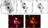 |
Fig. 1 Panel a: 12CO J = 3–2 line integrated between 80 and 120 km s−1, the contour levels are 130, 160, 196, 230, and 262 K km s−1. Panel b: 13CO J = 3–2 line integrated between 90 and 110 km s−1, the contour levels are 27, 41, 55, and 72 K km s−1. Panel c: C18O J = 3–2 line integrated between 90 and 110 km s−1 with contour levels of 5, 11, 16, 22, and 27 K km s−1. Panel d: three-color image toward G29.96−0.02 displaying the Spitzer-IRAC 8 μm emission in red, the Herschel-PACS 70 μm emission in green, and the radio continuum emission at 20 cm as extracted from the MAGPIS in blue. The numbers indicate the positions of some features described in the text. The black cross indicates the position of the known O-type star (Watson & Hanson 1997). Panel e: two-color image of the G29.96−0.02 region showing Spitzer-IRAC 8 μm emission in red and the emission at 850 μm obtained from SCUBA in green. |
2 Data
2.1 J = 2–1 line
We used 13CO and C18O J = 2–1 data observed with the IRAM 30 m telescope toward G29.96−0.02 by Carlhoff et al. (2013). The data cubes were obtained from the CDS1 and have an angular and spectral resolution of 11′′.7 and 0.15 kms−1, respectively. The intensity of the data is on the main-beam brightness temperature (Tmb) scale. As indicated by Carlhoff et al. (2013), the typical rms noise level of the spectra in units of Tmb is about 1 K for both isotopes.
2.2 J = 3–2 line
The 12CO, 13CO, and C18O J = 3–2 data were extracted from two public databases of observations performed with the 15 m James Clerck Maxwell Telescope (JCMT) in Hawaii. The 12CO J = 3–2 data were obtained from the CO High-Resolution Survey (COHRS) with an angular and spectral resolution of 14′′ and 1 km s−1 (Dempsey et al. 2013). The data of the other isotopes were obtained from the 13CO/C18O (J = 3–2) Heterodyne Inner Milky Way Plane Survey (CHIMPS), which have an angular and spectral resolution of 15′′ and 0.5 km s−1 (Rigby et al. 2016). The intensities of the two datasets are on the  scale, and the mean detector efficiency ηmb = 0.61 was used for 12CO, and ηmb = 0.72 for 13CO and C18O to convert
  into the main-beam brightness temperature (
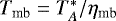 ; Buckle et al. 2009). The typical rms noise levels of the spectra, in units of
  , are 0.25, 0.35, and 0.40 K for 12CO, 13CO, and C18O, respectively. The data were visualized and analyzed with the Graphical Astronomy and Image Analysis Tool (GAIA)2 and with tools from the Starlink software package (Currie et al. 2014).
3 Presentation of G29.96−0.02
Figure 1 presents the massive star-forming region G29.96−0.02 as seen in different wavelengths. The molecular gas distribution related to G29.96−0.02 is presented in panels (a)–(c), where we show the integrated 12CO, 13CO, and C18O J = 3–2 emission, respectively. Figure 1d is a three-color image displaying the Spitzer-IRAC 8 μm emission in red, the Herschel-PACS 70 μm emission in green, and the radio continuum emission at 20 cm in blue as extracted from the New GPS of the Multi-Array Galactic Plane Imaging Survey (MAGPIS). Figure 1e displays in a two-color image the Spitzer-IRAC 8 μm and the SCUBA 850 μm emission in red and green, respectively. The emissions presented in panels d and e were selected in order to show the borders of the photodissociation regions (PDRs; displayed in the 8 μm emission), the distribution of the ionized gas (shown with the 20 cm emission), and the warm dust (70 μm emission). These are useful to indirectly and roughly discern features and their degree of ionization and warming by the UV radiation, together with the distribution of cold dust (displayed in the 850 μm emission). Numbers included in Figure 1d show the positions of some interesting objects for reference: (1) a UC H II region associated with a hot molecular cloud (Beuther et al. 2007), and the black cross indicates the location of its exciting O-type star (Watson & Hanson 1997), (2) an infrared dust cloud (better traced in the 850 μm emission in panel e; see Pillai et al. 2011), and (3) a massive YSO with molecular outflows (work in preparation). The linear size included in Fig. 1b and in subsequent figures in this work is derived by assuming a distance of 6.2 kpc to the analyzed molecular cloud.
4 Method and results
We used two methods to estimate 13CO and C18O column densities and X13∕18 (which is the ratio between them) throughout the molecular cloud depicted by the CO molecular emission (see Fig. 1a–c). In the following subsections we describe the two methods and their results.
4.1 LTE analysis
Assuming LTE, we estimated the column densities of 13CO and C18O pixel by pixel from the J = 3–2 emission. The optical depths ( and
and  ) and column densities (N(13CO) and N(C18O)), assuming a beam filling factor of 1, were derived using the following equations:
![Mathematical equation: \begin{equation*} \tau_{^{13}\textrm{CO}} = - \textrm{ln}\left(1 - \frac{T_{\textrm{mb}}({^{13}\textrm{CO}})}{15.87\left[\frac{1}{e^{15.87/T_{{\textrm{ex}}}}-1} - 0.0028\right]}\right),\end{equation*}](/articles/aa/full_html/2018/09/aa33658-18/aa33658-18-eq7.png) (1)
(1)
 (2)
(2)
with
 (3)
(3)
![Mathematical equation: \begin{equation*} \tau_{\textrm{C}}^{18}O = - \textrm{ln}\left(1 - \frac{T_{\textrm{mb}}(\textrm{C}^{18}O)}{15.81\left[\frac{1}{e^{15.81/T_{{\textrm{ex}}}}-1} - 0.0028\right]}\right),\end{equation*}](/articles/aa/full_html/2018/09/aa33658-18/aa33658-18-eq10.png) (4)
(4)
 (5)
(5)
with
 (6)
(6)
The J(Tex) parameter is  in the case of Eq. (3) and
  in Eq. (6). In all equations, Tmb is the peak main brightness temperature and Tex is the excitation temperature. Assuming that the 12CO J = 3–2 emission is optically thick, the Tex was derived from
![Mathematical equation: \begin{equation*} T_{{\textrm{ex}}} = \frac{16.6}{\textrm{ln}[1 + 16.6 / (T_{\textrm{peak}}(^{12}\textrm{CO}) + 0.036)]}.\end{equation*}](/articles/aa/full_html/2018/09/aa33658-18/aa33658-18-eq15.png) (7)
(7)
The 13CO and C18 O J = 3–2 emissions are optically thin throughout the analyzed molecular cloud. The average value of  obtained from the whole regionof the 13CO emission is 0.44, with a minimum of 0.17, and a maximum of 1.1. In the case of
  , we obtained an average of 0.13 with a minimum of 0.04 and a maximum of 0.45. Figure 2 presents the results obtained from the above expressions, displaying maps of Tex (left panel), N(13CO), and N(C18O) (middle and right panels), and for reference, contours of the integrated C18O J = 3–2 emission are included. Figure 3 displays a map of X13∕18 toward G29.96−0.02. Because the C18O line is weaker than the 13CO line and is even undetectable in some regions of the cloud where 13CO is detected, it is important to be cautious with unreal low values in N(C18O) that will yield artificially high values in X13∕18. Thus, only values above 5σ from the C18O integrated map were considered, which implies values above ~3 × 1015 cm−2 in the N(C18O) map.
Figure 4 displays a map of the integrated line ratio I13∕18 ( ), and Fig. 5 shows the abundance ratio X13∕18 versus the integrated line ratio I13∕18 obtained from all pixels of Figs. 3 and 4. From a linear fitting to the data of the X13∕18 vs. I13∕18 plot, we obtain A = 0.58 ± 0.08 and B = 2.80 ± 0.02 (Ax + B) with R2 =0.35 (red line in Fig. 5). Finally, Fig. 6 presents the relation between the abundance ratio and the C18O column density.
4.2 Non-LTE analysis
To estimate the column densities of 13CO and C18O, we used their J = 2–1 and J = 3–2 transitions and the RADEX code3 (van der Tak et al. 2007). The 13CO and C18O J = 2–1 data cubes were degraded to the angular and spectral resolution of the 13CO and C18O J = 3–2 data. Then, the spatial component of all cubes were rebinned to a 60 × 73 grid with pixels of about 11′′ in size.
The inputs of RADEX are the kinetic temperature (TK), the line velocity width at FWHM (Δ v), and the line peak temperature (Tpeak). The code fits the column and volume molecular densities (N and nH_2). For TK we assumed that the gas is coupled tothe dust (i.e., TK = Tdust), and we created a dust temperature map obtained from a spectral energy distribution (SED) using data from Herschel-PACS at 160 μm, Herschel-SPIRE at 250 and 350 μm, and SCUBAat 850 μm. The images at 160, 250, and 850 μm were convolved to the angular resolution of the Herschel-SPIRE 350 μm map (which has the coarsest angular resolution of all the used bands, this is 24′′) and rebinned to the same pixel size of the molecular lines data cubes. Then, fluxes at the four wavelengths were fit pixel by pixel with a modified blackbody curve,
 (8)
(8)
where Sν is the flux at the frequency ν, mH the hydrogen atom mass, μ = 2.8 by adopting a relative helium abundance of 25%, N(H2) the H2 column density, Bν is the Plank function,  is the dust opacity, where we adopt β = 2, and for a frequency ν0 = 1 THz and a gas-to-dust ratio of 100,
  cm2 g−1. The obtained dust temperature map (Fig. 7) shows almost the same results as presented in Carlhoff et al. (2013), who followed the same procedure, but without the 850 μm data. We included this wavelength in our SED with the aim of obtaining more accurate results toward the coldest regions. As an additional result obtained from this SED, we present in Fig. 8 the H2 column density map toward the region.
To obtain Δv and Tpeak pixel by pixel from the data cubes, we created maps of the second-moment and the emission peak for the 13CO and C18O J = 2–1 and J = 3–2 lines, respectively. Assuming Gaussian line profiles, the second-moment, which is the line velocity dispersion, was multiplied by a factor of 2.355 to obtain the FWHM Δv. The molecular data were convolved to the same angular resolution as the Tdust map (i.e., 24′′). Even though Carlhoff et al. (2013) pointed out that the velocity is rather homogeneous thorughout this cloud (W43-South in their paper), from our inspection of the data cubes we found that the central velocity and the line shape of the spectra change within the cloud. Thus, we selected four regions in which the spectra allowed us to obtain reliable FWHM Δ v maps. This is because if we integrate along a velocity range with a low signal-to-noise ratio (S/N), the second-moment can yield very high unrealistic values. The selected velocity ranges for each line in each region are presented in Table 1.
The N(13CO) and N(C18O) obtained from RADEX toward each region are presented in Figs. 9 and 10, respectively. There are several pixels for which RADEX does not yield any value (i.e., the code does not converge), mainly in the 13CO case. The reasons for this issue are discussed in the next section. Figure 11 displays the X13∕18 ratio obtained from the N(13CO) and N(C18O) maps.
 |
Fig. 2 Maps showing the results obtained from the 12CO, 13CO, and C18O J = 3–2 emission under the LTE assumption. Left panel: excitation temperature (Tex), the color baris in units of K. Middle and right panels: 13CO and C18O column densities, respectively. The color bars are in units of cm−2. Contours of the integrated C18O J = 3–2 emission are included for reference (same contours as presented in Fig. 1c). |
 |
Fig. 3 Map of the X13∕18 in the G29.96−0.02 region obtained from the 12CO, 13CO, and C18O J = 3–2 line assuming LTE. Contours of the integrated C18O J = 3–2 emission are included for reference. |
 |
Fig. 4 Map of the integrated line ratio I13∕18 in the G29.96−0.02 region. Contours of the integrated C18O J = 3–2 emission are included for reference. |
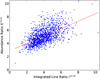 |
Fig. 5 Abundance ratio X13∕18 vs. integrated line ratio I13∕18 obtained from all pixels between Figs. 3 and 4. The red line is the result from a linear fitting. |
5 Discussion
Taking into account that G29.96−0.02 is located at a galactocentric distance of about 4.4 kpc (assuming a distance to the source of 6.2 kpc; Russeil et al. 2011), following the Wilson & Rood (1994) atomic relations, the X13∕18 ratio in this region should be about 7. From the LTE results, we have an X13∕18 average value of about 5, and as Fig. 3 shows, X13∕18 varies from about 1.5–10.5 throughout the studied region. For instance, toward the dark cloud (marked with 2 in Fig. 1d), the value of X13∕18 is low, about 3, which is consistent with the fact that it is a dense region that the UV radiation cannot penetrate to selectively photodissociate the C18O isotopes. Figure 12 displays the X13∕18 map obtained from the LTE assumption with contours of the radio continuum emission at 20 cm tracing the ionized gas. In general, the higher values of X13∕18 are located mainly at the borders, or close to them, of regions with ionized gas, where the far-UV photons are likely escaping and selectively photodissociate the C18O species, as found in previous works (e.g., Shimajiri et al. 2014; Kong et al. 2015; Areal et al. 2018). This is the case in the northeastern region of the UC H II region, where many pixels have high X13∕18 values (about 8), while toward the southwest, in coincidence with a dark cloud, X13∕18 is low (about 3). This spatial distribution suggests that the radiation of the UC H II region mainly escapes toward the northeast, photodissociating the gas, while toward the west and southwest, it stalls in a dense clump that is traced by the dust emission at 850 μm, and it heats the hot core (Beuther et al. 2007). The same phenomenon may occur in the largest radio continuum feature that lies almost at the center in Fig. 12. As described above, toward the northeast, the UV radiation encounters a very dense component (the dark cloud) that prevents the C18O photodissociation. The same may occur toward the southwest, while the far-UV photons likely escape toward the other borders. Figure 6 shows that X13∕18 decreases with the increase of N(C18O). Considering that in general high N(C18O) implies high extinction (AV), the result displayed in this figure supports that the far-UV radiation cannot penetrate the inner parts of the clouds (dark clouds), as described above. Even though we have to be careful with the relation between N(C18O) and AV because the C18O may be selectively photodissociated in some regions and hence it does not accurately relate to AV, the tendency displayed in Fig. 6 is indeed clear.
From the comparison between the maps of the abundance and the integrated line ratios (Figs. 3 and 4), which compares values that were derived from excitation considerations (LTE assumption) with values that are direct measurements, it can be appreciated that both parameters present the same behavior across the region. Areal et al. (2018) found linear relations between X13∕18 and I13∕18 that slightlyvaried among YSOs, H II, and diffuse H II regions. In this case, a linear tendency can be suggested (see Fig. 5) but with a large dispersion, which shows that very different physical conditions are present in the gaseous component throughout the studied cloud.
The results from RADEX do not cover the whole region as in the LTE case, but we can still obtain valuable information from them. First, the column densities values are higher than those obtained in the LTE assumption, which is somewhat expected because it isknown that LTE column densities of molecular clouds typically underestimate the true column densities by factors ranging from 1 to 7 (Padoan et al. 2000).
In the case of C18O, RADEX yields results in almost all pixels of the studied regions, and as Fig. 10 shows, the obtained N(C18O) toward the selected regions presents similar features as in the N(C18O) LTE map. In the 13CO case, there are several pixels for which RADEX does not yield any value, that is, pixels where the code does not converge. However, pixels with results tend to show similar morphological features as in the N(13CO) LTE map. For the blanked pixels, this is not a useless result, on the contrary, the non-convergence of the RADEX code can give us important information about the physical conditions in the region. Analyzing what happens with RADEX in these pixels, we found that there are two types of non-convergence: (i) the code does not fit the inputs (Tpeak, Δ v, and TK) for one or both lines, and (ii) while the inputs of both lines are fit, the ratio between them is not.
Taking into account that we had assumed that TK = Tdust, it is possible that the first case of non-convergence may imply that the gas is not coupled to the dust, mainly in the gaseous component traced mostly by the 13CO, and thus they have different temperatures. Certainly, we tested other values of TK, and we observed that for values higher than Tdust, RADEX gives good results. The second type of non-convergence may indicate that the J = 2–1 and J = 3–2 transitions arise from different components at different temperatures, or even a more complicate phenomenon: for example, it could be that a part of the J = 3–2 transition arises from a colder component, while another part of the emission arises from a hotter one, that is, a two-component RADEX solution (see Paron et al. 2016, where this was assumed for the J = 3–2 transition toward an H II region in the Large Magellanic Cloud). Thus, the non-convergence of RADEX shows the complexity of the region, and suggests that the molecular gas is indeed under different physical conditions, not only spatially throughout the cloud, but also along the line of sight.
Considering the above discussion, the X13∕18 values obtained from RADEX (see Fig. 11) are in general practically meaningless. Only toward the northeast of R2 and southwest of R4 (where both regions overlap) is X13∕18 quite constant, with values similar to those obtained in the LTE case. This region coincides with the dark cloud (marked with 2 in Fig. 1d), in which the physical conditions may indeed be quite constant.
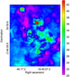 |
Fig. 7 Dust temperature derived from three Herschel bands (160, 250, and 350 μm) and the SCUBA band at 850 μm. Contours of the integrated C18O J = 3–2 emission are included for reference. The color bar is in units of K. |
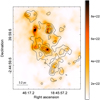 |
Fig. 8 H2 column density derived from three Herschel bands (160, 250, and 350 μm) and the SCUBA band at 850 μm. The color bar is in units of cm−2. Contours of the integrated C18O J = 3–2 emission are included for reference. |
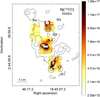 |
Fig. 9 13CO column density obtained from the RADEX code toward the analyzed regions. The color bar is in units of cm−2. Contours of the integrated C18O J = 3–2 emission are included for reference. |
Velocity ranges in km s−1 of the selected regions from which second-moment and emission peak maps were obtained.
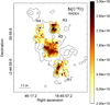 |
Fig. 10 C18O column density obtained from the RADEX code toward the analyzed regions. The color bar is in units of cm−2. Contours of the integrated C18O J = 3–2 emission are included for reference. |
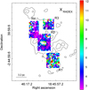 |
Fig. 11 X13∕18 abundance ratio obtained from the RADEX code toward the analyzed regions. Contours of the integrated C18O J = 3–2 emission are included for reference. |
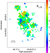 |
Fig. 12 Map of the X13∕18 obtained under theLTE assumption with contour of the radio continuum emission with levels of 15, 40, and 65 mJy beam−1. The angular resolution of the radio continuum data is about 5′′.5. |
Beam-filling factor effects
It is important to mention that our results are based on the assumption that the beam-filling factor of the 13CO and C18O emission is equal to 1, which corresponds to molecular features that completely fill the telescope beam. This is not completely true because the clouds are usually structured on the subparsec scale, implying beam-filling factors lower than the unity. We investigated the influence that, on average, a possible beam dilution effect could have in the obtained X13∕18. According to Kim et al. (2006), we can estimate the beam filling factor as  , where
  and
and  are the source and beam sizes, respectively. The effective beam size of 13 CO and C18O J = 3–2 data is about 15′′, which corresponds to 0.45 pc at the considered distance of 6.2 kpc. Using data from Herschel-PACS 70 μm (angular resolution ~5′′), we determined that the sizes of dense cores and/or clumps in the region are expected to exceed 0.7 pc. Thus, the beam-filling factor of the molecular data is expected to exceed 0.7. Assuming that the 13CO emission likely traces more extended molecular components than the C18O emission, we considered the limit case in which
  and
and  . Thus, the obtained X13∕18 could be overestimated by up to 30%.
The beam-dilution effect would be less important in regions of diffuse gas than in those where the gas is clumpy. Diffuse gas regions are, in general, more exposed to far-UV radiation and therefore tend to have higher values of X13∕18, while the densest or clumpy regions are expected to have lower values of X13∕18. Thus, the beam-dilution correction, applied mainly to the C18O in clumpy regions, would tend to decrease the X13∕18 value in the densest regions, which would highlight the behavior of X13∕18 found throughout the cloud even more strongly.
6 Summary and concluding remarks
Using the 12CO, 13CO, and C18O J = 3–2, and 13CO and C18O J = 2–1 emission, we studied the column densities and the 13CO/C18O abundance ratio (X13∕18) distribution toward the high-mass star-forming region G29.96−0.02 with LTE and non-LTE methods.
From the LTE analysis we found an X13∕18 average value of about 5 that varied from about 1.5 to 10.5 across the studied region. This shows that in addition to the dependency between X13∕18 and the galactocentric distance, local physical conditions greatly influence this abundance ratio. Moreover, these results show that if a value of X13∕18 needs to be used, it is better to obtain it from the direct molecular observations (if these are available) than from indirect estimates of elemental abundances.
Our analysis of the variation in the X13∕18 value across the molecular cloud shows that close to regions of ionized gas, X13∕18 tends to increase, in complete agreement with the selective far-UV C18O dissociation found in other works. Additionally, the analysis of the spatial distribution between the X13∕18 map, the ionized regions, and the dark clouds allows us to suggest in which regions the radiation is stalled in dense gaseous components, and in which regions it escapes and selectively photodissociates the C18O species. This roughly maps the degree of far-UV irradiation in different molecular components.
The non-LTE analysis based on the RADEX code proves that the region is indeed very complex, showing that the molecular gas may have very different physical conditions, not only spatially throughout the cloud, but also along the line of sight. We found that in some cases the non-convergence of RADEX can show when the assumption fails that gas and dust are thermally coupled, which would define a quite accurate lower limit for the kinetic temperature of the molecular gas.
Finally, it is important to note that this type of studies may represent a tool for indirectly estimating from molecular line observationsthe degree of photodissociation in molecular clouds, which is very useful to study many chemical chains occurring in such interstellar environments.
Acknowledgments
We thank the anonymous referee for their helpful comments and suggestions. M.B.A. is a doctoral fellow of CONICET, Argentina. S.P. and M.O. are members of the Carrera del Investigador Científico of CONICET, Argentina. This work was partially supported by Argentina grants awarded by UBA (UBACyT), CONICET, and ANPCYT.
References
- Areal, M. B., Paron, S., Celis Peña, M., & Ortega, M. E. 2018, A&A, 612, A117 [NASA ADS] [CrossRef] [EDP Sciences] [Google Scholar]
- Beltrán, M. T., Olmi, L., Cesaroni, R., et al. 2013, A&A, 552, A123 [NASA ADS] [CrossRef] [EDP Sciences] [Google Scholar]
- Beuther, H., Zhang, Q., Bergin, E. A., et al. 2007, A&A, 468, 1045 [NASA ADS] [CrossRef] [EDP Sciences] [Google Scholar]
- Buckle, J. V., Hills, R. E., Smith, H., et al. 2009, MNRAS, 399, 1026 [NASA ADS] [CrossRef] [Google Scholar]
- Carlhoff, P., Nguyen Luong, Q., Schilke, P., et al. 2013, A&A, 560, A24 [NASA ADS] [CrossRef] [EDP Sciences] [Google Scholar]
- Cesaroni, R., Churchwell, E., Hofner, P., Walmsley, C. M., & Kurtz, S. 1994, A&A, 288, 903 [NASA ADS] [Google Scholar]
- Currie, M. J., Berry, D. S., Jenness, T., et al. 2014, in Astronomical Data Analysis Software and Systems XXIII, ed. N. Manset, & P. Forshay, ASP Conf. Ser., 485, 391 [NASA ADS] [Google Scholar]
- Dempsey, J. T., Thomas, H. S., & Currie, M. J. 2013, ApJS, 209, 8 [NASA ADS] [CrossRef] [Google Scholar]
- Kim, S.-J., Kim, H.-D., Lee, Y., et al. 2006, ApJS, 162, 161 [NASA ADS] [CrossRef] [Google Scholar]
- Kong, S., Lada, C. J., Lada, E. A., et al. 2015, ApJ, 805, 58 [NASA ADS] [CrossRef] [Google Scholar]
- Lada, C. J., Lada, E. A., Clemens, D. P., & Bally, J. 1994, ApJ, 429, 694 [NASA ADS] [CrossRef] [Google Scholar]
- Lin, S.-J., Shimajiri, Y., Hara, C., et al. 2016, ApJ, 826, 193 [NASA ADS] [CrossRef] [Google Scholar]
- Olmi, L., Cesaroni, R., Hofner, P., et al. 2003, A&A, 407, 225 [NASA ADS] [CrossRef] [EDP Sciences] [Google Scholar]
- Padoan, P., Juvela, M., Bally, J., & Nordlund, Å. 2000, ApJ, 529, 259 [NASA ADS] [CrossRef] [Google Scholar]
- Paron, S., Ortega, M. E., Fariña, C., et al. 2016, MNRAS, 455, 518 [NASA ADS] [CrossRef] [Google Scholar]
- Pillai, T., Kauffmann, J., Wyrowski, F., et al. 2011, A&A, 530, A118 [NASA ADS] [CrossRef] [EDP Sciences] [Google Scholar]
- Rigby, A. J., Moore, T. J. T., Plume, R., et al. 2016, MNRAS, 456, 2885 [NASA ADS] [CrossRef] [Google Scholar]
- Russeil, D., Pestalozzi, M., Mottram, J. C., et al. 2011, A&A, 526, A151 [NASA ADS] [CrossRef] [EDP Sciences] [Google Scholar]
- Shimajiri, Y., Kitamura, Y., Saito, M., et al. 2014, A&A, 564, A68 [NASA ADS] [CrossRef] [EDP Sciences] [Google Scholar]
- Townsley, L. K., Broos, P. S., Garmire, G. P., et al. 2014, ApJS, 213, 1 [NASA ADS] [CrossRef] [Google Scholar]
- van der Tak, F. F. S., Black, J. H., Schöier, F. L., Jansen, D. J., & van Dishoeck E. F. 2007, A&A, 468, 627 [NASA ADS] [CrossRef] [EDP Sciences] [Google Scholar]
- Watson, A. M., & Hanson, M. M. 1997, ApJ, 490, L165 [NASA ADS] [CrossRef] [Google Scholar]
- Wilson, T. L., & Rood, R. 1994, ARA&A, 32, 191 [NASA ADS] [CrossRef] [Google Scholar]
- Wood, D. O. S., & Churchwell, E. 1989, ApJS, 69, 831 [NASA ADS] [CrossRef] [Google Scholar]
GAIA is a derivative of the Skycat catalog and image display tool, developed as part of the VLT project at ESO. Skycat and GAIA are free software under the terms of the GNU copyright.
RADEX is a statistical equilibrium radiative transfer code, available as part of the Leiden Atomic and Molecular Database (http://www.strw.leidenuniv.nl/~moldata/).
All Tables
Velocity ranges in km s−1 of the selected regions from which second-moment and emission peak maps were obtained.
All Figures
|
Fig. 1 Panel a: 12CO J = 3–2 line integrated between 80 and 120 km s−1, the contour levels are 130, 160, 196, 230, and 262 K km s−1. Panel b: 13CO J = 3–2 line integrated between 90 and 110 km s−1, the contour levels are 27, 41, 55, and 72 K km s−1. Panel c: C18O J = 3–2 line integrated between 90 and 110 km s−1 with contour levels of 5, 11, 16, 22, and 27 K km s−1. Panel d: three-color image toward G29.96−0.02 displaying the Spitzer-IRAC 8 μm emission in red, the Herschel-PACS 70 μm emission in green, and the radio continuum emission at 20 cm as extracted from the MAGPIS in blue. The numbers indicate the positions of some features described in the text. The black cross indicates the position of the known O-type star (Watson & Hanson 1997). Panel e: two-color image of the G29.96−0.02 region showing Spitzer-IRAC 8 μm emission in red and the emission at 850 μm obtained from SCUBA in green. |
| In the text | |
|
Fig. 2 Maps showing the results obtained from the 12CO, 13CO, and C18O J = 3–2 emission under the LTE assumption. Left panel: excitation temperature (Tex), the color baris in units of K. Middle and right panels: 13CO and C18O column densities, respectively. The color bars are in units of cm−2. Contours of the integrated C18O J = 3–2 emission are included for reference (same contours as presented in Fig. 1c). |
| In the text | |
|
Fig. 3 Map of the X13∕18 in the G29.96−0.02 region obtained from the 12CO, 13CO, and C18O J = 3–2 line assuming LTE. Contours of the integrated C18O J = 3–2 emission are included for reference. |
| In the text | |
|
Fig. 4 Map of the integrated line ratio I13∕18 in the G29.96−0.02 region. Contours of the integrated C18O J = 3–2 emission are included for reference. |
| In the text | |
|
Fig. 5 Abundance ratio X13∕18 vs. integrated line ratio I13∕18 obtained from all pixels between Figs. 3 and 4. The red line is the result from a linear fitting. |
| In the text | |
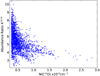 |
Fig. 6 Abundance ratio X13∕18 vs. the C18O column density obtained from all pixels of Fig. 3. |
| In the text | |
|
Fig. 7 Dust temperature derived from three Herschel bands (160, 250, and 350 μm) and the SCUBA band at 850 μm. Contours of the integrated C18O J = 3–2 emission are included for reference. The color bar is in units of K. |
| In the text | |
|
Fig. 8 H2 column density derived from three Herschel bands (160, 250, and 350 μm) and the SCUBA band at 850 μm. The color bar is in units of cm−2. Contours of the integrated C18O J = 3–2 emission are included for reference. |
| In the text | |
|
Fig. 9 13CO column density obtained from the RADEX code toward the analyzed regions. The color bar is in units of cm−2. Contours of the integrated C18O J = 3–2 emission are included for reference. |
| In the text | |
|
Fig. 10 C18O column density obtained from the RADEX code toward the analyzed regions. The color bar is in units of cm−2. Contours of the integrated C18O J = 3–2 emission are included for reference. |
| In the text | |
|
Fig. 11 X13∕18 abundance ratio obtained from the RADEX code toward the analyzed regions. Contours of the integrated C18O J = 3–2 emission are included for reference. |
| In the text | |
|
Fig. 12 Map of the X13∕18 obtained under theLTE assumption with contour of the radio continuum emission with levels of 15, 40, and 65 mJy beam−1. The angular resolution of the radio continuum data is about 5′′.5. |
| In the text | |
Current usage metrics show cumulative count of Article Views (full-text article views including HTML views, PDF and ePub downloads, according to the available data) and Abstracts Views on Vision4Press platform.
Data correspond to usage on the plateform after 2015. The current usage metrics is available 48-96 hours after online publication and is updated daily on week days.
Initial download of the metrics may take a while.