| Issue |
A&A
Volume 617, September 2018
|
|
|---|---|---|
| Article Number | A43 | |
| Number of page(s) | 14 | |
| Section | Planets and planetary systems | |
| DOI | https://doi.org/10.1051/0004-6361/201832922 | |
| Published online | 12 September 2018 | |
Dynamics of nanodust particles emitted from elongated initial orbits
1
Space Research Centre, Polish Academy of Sciences,
Bartycka 18A,
00-716
Warsaw, Poland
e-mail: This email address is being protected from spambots. You need JavaScript enabled to view it.
2
Department of Physics and Technology, UiT: The Arctic University of Norway,
Postboks 6050 Langnes,
9037
Tromso, Norway
e-mail: This email address is being protected from spambots. You need JavaScript enabled to view it.
Received:
28
February
2018
Accepted:
30
May
2018
Abstract
Context. Because of high charge-to-mass ratio, the nanodust dynamics near the Sun is determined by interplay between the gravity and the electromagnetic forces. Depending on the point where it was created, a nanodust particle can either be trapped in a non-Keplerian orbit, or escape away from the Sun, reaching large velocity. The main source of nanodust is collisional fragmentation of larger dust grains, moving in approximately circular orbits inside the circumsolar dust cloud. Nanodust can also be released from cometary bodies, with highly elongated orbits.
Aims. We use numerical simulations and theoretical models to study the dynamics of nanodust particles released from the parent bodies moving in elongated orbits around the Sun. We attempt to find out whether these particles can contribute to the trapped nanodust population.
Methods. We use two methods: the motion of nanodust is described either by numerical solutions of full equations of motion, or by a two-dimensional (heliocentric distance vs. radial velocity) model based on the guiding-center approximation. Three models of the solar wind are employed, with different velocity profiles. Poynting–Robertson and the ion drag are included.
Results. We find that the nanodust emitted from highly eccentric orbits with large aphelium distance, like those of sungrazing comets, is unlikely to be trapped. Some nanodust particles emitted from the inbound branch of such orbits can approach the Sun to within much shorter distances than the perihelium of the parent body. Unless destroyed by sublimation or other processes, these particles ultimately escape away from the Sun. Nanodust from highly eccentric orbits can be trapped if the orbits are contained within the boundary of the trapping region (for orbits close to ecliptic plane, within ~0.16 AU from the Sun). Particles that avoid trapping escape to large distances, gaining velocities comparable to that of the solar wind.
Key words: Sun: heliosphere / solar wind / acceleration of particles / interplanetary medium / comets: general
© ESO 2018
1 Introduction
The distribution and dynamics of interplanetary dust in the vicinity of the Sun is important for understanding the evolution of the interplanetary dust cloud as a whole and its interactions with the solar wind (see e.g., Mann et al. 2014). Near the Sun, the dust cloud number densities and collision rates are the highest. The dust production and destruction rates vary with solar activity, for example, the coronal mass ejections (Ragot & Kahler 2003). Dust destruction by mutual collisions is the main source of small (sub-micrometer) dust particles. Dust collisions are probably also the largest dust-related source of heavy pick-up ions in the solar wind (Mann & Czechowski 2005). The small dust particles are pushed away from the Sun by radiation pressure and electromagnetic forces and form an outward-directed flux of dust in the interplanetary medium. The dust particles of sizes of a few nanometers can be accelerated to speeds of the order of the solar wind speed (Mann et al. 2007; Czechowski & Mann 2010, 2011, 2012).
Dust particles of micrometer and smaller sizes are observed in situ by space-based dust instruments. However, dust impacts can also be observed by other methods. In particular, the dust can be detected by plasma wave measurements, because the dust impacts generate free charges and change the electric potential of the spacecraft. Recent examples of dust studies relying on plasma wave measurements are STEREO, Cassini, and Wind (e.g., Meyer-Vernet et al. 2009; Malaspina et al. 2014; Kellogg et al. 2016) observations. NASA’s Parker Solar Probe (Fox et al. 2016) and ESA’s Solar Orbiter (Mueller et al. 2013) mission will, in the near future, explore the vicinity of the Sun. They both carry instruments for field measurements (see Bale et al. 2016) and have the potential to detect dust impacts.
The nanodust particles are of particular interest because, due to the large value of their charge-to-mass ratio, their dynamics is largely determined by electromagnetic forces. In our previous work on nanodust dynamics (Czechowski & Mann 2010, 2012), we considered the nanodust created by collisional fragmentation of larger grains belonging to the circumsolar dust cloud in the vicinity of the Sun. The initial velocity of nanodust particles was consequently assumed to be close to that of a circular Keplerian orbit. We found that the majority of nanodust particles created near the ecliptic within a critical radius of ~0.16 AU from the Sun would then be trapped in non-Keplerian orbits determined by the interplay between gravitation and electromagnetic forces. Away from the ecliptic, the size of the trapping region depends on the release point on the orbit. The particles created outside the trapping region escape away from the Sun, reaching a high velocity, comparable to that of the solar wind.
In the present work, we consider the more general case of nanodust released from elongated orbits, in particular the highly eccentric orbits, like those of the cometary bodies passing close to the Sun.
Comets release gas and dust particles due to illumination by the Sun. The dust particles are carried and accelerated in the outflowing coma gas. Observations suggest that dust properties vary within the coma, most likely due to fragmentation, sublimation of volatiles, and other unknown effects.
There is little information about the smallest size of the dust, because astronomical observations are typically limited to sizes of ~100 nm and larger. An exception is provided by X-ray observations, which are capable of identifying nanodust. Analyzing X-ray observationsof comets, Snios et al. (2014) derived the upper limits on the nanodust contribution. There is also some positive evidence for the presence of nanodust near comets. The in situ detection of nanodust was reported from space missions to P/Halley (Utterback & Kissel 1990, 1995).
These observations were in line with the assumption that the nanodust forms during fragmentation events, but the formation of nanodust during fragmentation is not well explored (see e.g., Mann 2017). Szego et al. (2014) predicted that Rosetta will detect nano dust at comet 67P/Churyumov–Gerasimenko. There is no instrument onboard that was specifically designed for detecting nanodust, and, so far, there is only little evidence.
Burch et al. (2015) report that the ion and electron instrument RPC/IES detects negative particles at energies from about 100 eV/q to more than 18 keV/q and interpret these observations as clusters of molecules with diameters of less than 100 nm that reach the spacecraft from the direction of the comet and from the direction of the Sun. Gombosi et al. (2015) describe the trajectories in detail and show that the nanodust flux at Rosetta could be intermittent. Alternatively, one could speculate that the impacts from the sunward direction that RPC/IES observes are from minor solar wind constituents, as, for example, negative oxygen ions have energies of around 10 keV (cf. Mann 2017).
In our simulations, we restrict attention to dynamics of the (hypothetical) nanodust created in eccentric orbits at zero initial velocity relative to the parent body. We only consider the behavior of nanodust after it is released; the production mechanism of nanodust is beyond the scope of this study. We show that a high value of eccentricity combined with a large aphelium distance, typical for the release from a comet, eliminates the possibility of trapping. In the rare case that the dust in the initial orbit does not extend outside the limits of the trapping region (~0.16 AU near the ecliptic; see Czechowski & Mann 2010, 2012), a particle emitted near the aphelium can be trapped for arbitrarily high eccentricity.
The nanodust particles emitted from an elongated orbit follow trajectories that are very different from those of larger dust grains with smaller charge-to-mass ratios. In particular, some of the nanodust particles emitted from the inbound part of the orbit may approach the Sun to distances much smaller than the parent body perihelium.
The plan of the paper is as follows. In Sect. 2, we briefly present the equations of motion and our solar wind models. Section 3 describes our recent development of the phase space model based on the guiding center approximation (see Czechowski & Mann 2010, 2012 for the earlier version). Section 4 presents our results for dynamics of nanodust particles emitted from parent bodies moving in elongated Keplerian orbits; it includes subsections dealing with trapping conditions, trapping of nanodust emitted from the perihelium, and dynamics of particles released at an arbitrary point on the parent-body orbit. Our conclusions are given in Sect. 5.
2 Simulations of nanodust propagation in the solar wind
Our model of the solar wind and the solar magnetic field is very simple. The solar wind velocity is radially directed, and the magnetic field has the form of the Parker spiral. Distinct from our previous work, the solar wind speed can depend on the heliocentric distance. The motion of the nanodust particles is studied by means of the straightforward numerical simulation. We also use the two-dimensional (2D) phase space model derived from the leading order of the guiding center approximation. The 2D model describes the motion of the nanodust particle in the (r, v) plane, where r is the heliocentric distance and v the radial component of the particle velocity, and provides a good approximation to our numerical results for particles with large enough values (10−5 –10−4 e/mp) of the charge-to-mass ratio. We found the model helpful for qualitative understanding of the dynamics of nanodust.
2.1 Equations of motion
The equation of motion for the nanodust particle has the form
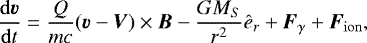 (1)
(1)
where Fγ is the radiation force:
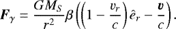 (2)
(2)
We assume the radiation pressure to gravity ratio β for nanodust particles to be small (β = 0.1; see Czechowski & Mann 2010, 2012). In some calculations, we replace Fγ by (GMsβ∕r2)êr, that is, we neglect the tangential (Poynting–Robertson drag) force.
In some of our simulations, we include Fion, the drag force caused by solar wind proton impacts on a grain:
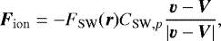 (3)
(3)
where FSW(r) = nSW(r)mp|v −V|2 is the solar wind proton flux at r relative to dust grain, and CSW,p is given by (Minato et al. 2004):
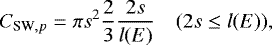 (4)
(4)
![Mathematical equation: \begin{equation*} C_{{\textrm{SW},p}}=\pi s^2 \left[1-\frac{1}{3}\left(\frac{l(E)}{2s}\right)^2\right]\ \ \ (2s > l(E)).\end{equation*}](/articles/aa/full_html/2018/09/aa32922-18/aa32922-18-eq5.png) (5)
(5)
Here, s is the radius of the grain, and l(E) is the range of a proton of initial energy E = (1∕2)mp|v −V|2 passing through the material of the grain. Following Minato et al. (2004), we assume l(E) ∝ E1∕2 with l(1 keV) = 0.092 μm for silicate grains. Similar to Minato et al. (2004), we simplify the proton drag force by neglecting the thermal component of the proton velocity. In our simulations, the proton drag force becomes important only in the immediate vicinity of the Sun, where the proton number density is high.
We assume that the charge to mass ratio Q∕m of the nanodust particle is constant during the motion. In the region within 1 AU from the Sun, the characteristic time for charge fluctuations for nanodust is short relative to the Larmor rotation time (Czechowski & Mann 2010, 2012). The surface charge on the grain can then be approximated by the equilibrium charge, which, based on theoretical estimations (Mukai 1981; Kimura & Mann 1998), can be taken to be approximately constant within our region of calculations.
2.2 Solar wind models
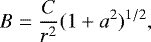
The solar wind flow velocity V we assume to be radially directed and independent of time. Distinct from our previous work (Czechowski & Mann 2010, 2012), we allow the solar wind speed V to depend on the heliocentric distance r: V = V (r). The magnetic field B has the form of the Parker spiral:
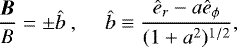 (6)
(6)
 (7)
(7)
 (8)
(8)
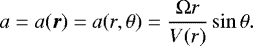
Here Ω is the angular rotation speed of the Sun, θ the heliographic colatitude, êr, êϕ, and êθ denote the unit vectors of the heliographic inertial coordinate system. The constant C can be written as  , where
  is the absolute value of the radial component of B at the reference distance
  . The constant C in Eq. (7) can in general be different for different field lines. As in our previous work (Czechowski & Mann 2010, 2012), we use two values for
  at
at  = 1 AU, one for the slow (35 μG) and one for the fast (45 μG) solar wind region. We note that our present definition of a (Eq. (8)) differs from that used in Czechowski & Mann (2010) in that we include the factor of r.
Our model includes the heliospheric current sheet and the two-component (slow and fast) solar wind structure. The current sheet is included by assuming that the rotating solar surface is divided into two hemispheres with opposite field polarity. The boundary between the hemispheres (the magnetic equator) is approximated by a great circle at a fixed tilt relative to the solar equator. In most of the calculations reported here, the tilt was set to 20°.
The magnetic field polarity in our simulations corresponds to outgoing (positive) field in the northern solar hemisphere. This is known as “defocusing” or “qA > 0” polarity, with the electric field − (1∕c)V ×B induced by the plasma motion pointing away from the current sheet. The motion of particles with positive charge in our “defocusing”field model is equivalent to that of negatively charged particles in the “focusing” field. To simulate the motion of Q > 0 particles in the “focusing” field, we therefore use Q < 0 particles without changing our magnetic field model.
We consider three different models of the solar wind (Fig. 1). In all of them, the solar wind velocity is radially directed. The models differ by the assumed solar wind speed dependence on the heliocentric distance r. Model 1 is the same as used in our previous work (Czechowski & Mann 2010, 2012), with r-independent speed: V = 400 km s−1 for the slow and V = 800 km s−1 for the fast solar wind. In some calculations we use the same (slow) solar wind speed for all heliographic latitudes.
The other two models (models 2 and 3) are used as test cases of the r-dependent solar wind speed. We do not propose these models as realistic descriptions of the solar wind: our aim is to test the influence of the different V (r) profiles on nanodust dynamics. In model 2, the function V (r) is given by the analytic formula ![Mathematical equation: $V(r)=V_2\equiv[2A(r-r_a)]^{1/2}$](/articles/aa/full_html/2018/09/aa32922-18/aa32922-18-eq14.png) (A = 3.4 m s−2, ra = –0.6 RSun), obtained by Sheeley et al. (1997) as a fit to one of the observed solar plasma velocity profiles. Although these observations were restricted to the vicinity of the Sun, we use the same formula also beyond this region. Model 3 is defined by V (r) = V2(r)∕(1 + V2(r)∕(800 km s^-1)): we use it as an example of the solar wind with a steep velocity profile near the solar surface and approximately constant speed near 1 AU. The fast wind velocity is equal to V (r) multiplied by two. In all our models, the fast solar wind region is limited to heliographic latitudes higher than the tilt angle.
(A = 3.4 m s−2, ra = –0.6 RSun), obtained by Sheeley et al. (1997) as a fit to one of the observed solar plasma velocity profiles. Although these observations were restricted to the vicinity of the Sun, we use the same formula also beyond this region. Model 3 is defined by V (r) = V2(r)∕(1 + V2(r)∕(800 km s^-1)): we use it as an example of the solar wind with a steep velocity profile near the solar surface and approximately constant speed near 1 AU. The fast wind velocity is equal to V (r) multiplied by two. In all our models, the fast solar wind region is limited to heliographic latitudes higher than the tilt angle.
For calculations including the proton drag force, we also need the proton density profile np (r) (Fig. 1, bottom panel). We assume that this is given by (for the slow wind component) 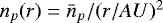 (model 1) and by np(r) = npcV (rc)∕V (r)
  (models 2 and 3), where
  . We take
  = 8 cm−3, rc = 0.16 AU (model 2) and 0.6 AU (model 3). We assume the same ram pressure for the slow and the fast solar wind: consequently, the proton density in the fast wind is assumed equal to one quarter of the slow wind value at the same heliocentric distance.
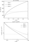 |
Fig. 1 Solar wind speed (upper panel) and the proton density (bottom panel) profiles used in our simulations (the slow wind component). The models 1, 2, and 3 are presented by the dotted, solid, and dashed lines, respectively. For the fast wind, the speed should be multiplied by 2, and the density divided by 4. |
3 Phase space model of nanodust dynamics in the solar wind
In addition to numerical solutions of Eq. (1), we use a new version of the 2D dynamical model derived in Czechowski & Mann (2010) from the guiding center approximation. The model describes the motion of the particle on the (r, vr) phase plane and has been shown to agree with the projections of the trajectories obtained from the full equation Eq. (1). The new version of the model permits the use of the r-dependent solar wind velocity and is not restricted to the r ≪ 1 AU region. The additional advantage is a simple expression for the constant of motion of the model.
The model is derived from the guiding center approximation (Northrop 1958). In the time-stationary case, the equation for the parallel component  of the velocity of the guiding center takes the form
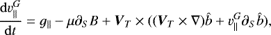 (9)
(9)
where g|| is the component of the gravity force (which we modify by the (1 − β) factor to account for the radiation force) per unit mass parallel to  , VT is the perpendicular part of the plasma velocity,
  and
and  is the adiabatic invariant, with
  being the perpendicular speed of the particle in the plasma frame.
In the leading order of the guiding center approximation, assuming zero electric field in the plasma frame, the perpendicular motion of the guiding center is given by
 (10)
(10)
Since for a purely radial V and  , VT has no component in the êθ direction, the guiding center motion by Eq. (10) is confined to the θ = const. cone. In the following, we use this fact to simplify the notation: we therefore write a(r), W(r), and so on, instead of a(r, θ) and W(r, θ), with implicit assumption that the value of θ is the same for all terms in the equation.
Evaluating the terms in Eq. (9) with use of Eqs. (6)–(8), and expressing  in terms of the radial velocity v of the guiding center (Czechowski & Mann 2011, 2012),
 (11)
(11)
and we obtain the two equations defining a dynamical system in the (r, v) phase plane:
 (12)
(12)
 (13)
(13)
The function W(r) is given by
 (14)
(14)
The three terms in W(r) correspond to the first three terms on the right-hand side of Eq. (9). The first two represent the parallel gravity and the magnetic mirror force, respectively. The third term can be regarded as the centrifugal force related to the rotation of the magnetic field line along which the guiding center moves (Czechowski & Mann 2010).
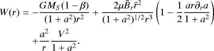
W(r) can also be written as
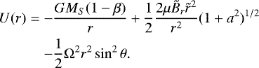
![Mathematical equation: \begin{eqnarray*} W(r)&=&\frac{GM_S(1-\beta)}{(1+a^2)r^2} \nonumber \\ &&\times\left[-1+\frac{r_2}{r}(1+a^2)^{1/2} \left(1-\frac{1}{2}\frac{ar\partial_r a}{1+a^2}\right) +\frac{r^3}{r_1^3}\right],\end{eqnarray*}](/articles/aa/full_html/2018/09/aa32922-18/aa32922-18-eq32.png) (15)
(15)
where 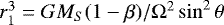 and r2 =
 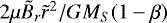 .
.
The system Eqs. (12) and (13) has a constant of motion
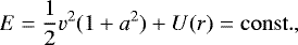 (16)
(16)
where
 (17)
(17)
We note that W(r) = −dU∕dr∕(1 + a2).
The conservation law Eq. (16) provides a simple analytical expression for the trajectory v(r). Figures 3 and 4 show how the results agree with the numerical solutions of the full equations of motion for nanodust particles.
In the slow solar wind, the parameter a(r) is of the order of 1 at 1 AU. For r ≪ 1 AU, a2 and, unless V (r) is very steep as r → 0, also ar∂ra, can be taken to be ≪1, so that Eq. (15) simplifies to
![Mathematical equation: \begin{equation*} W(r)=\frac{GM_S(1-\beta)}{r^2} \left[-1+\frac{r_2}{r}+\left(\frac{r}{r_1}\right)^3\right].\end{equation*}](/articles/aa/full_html/2018/09/aa32922-18/aa32922-18-eq37.png) (18)
(18)
We note that this expression for W(r) is independent of V (r). The somewhat unexpected consequence is that the particle dynamics in the (r, v) plane is, at r ≪ 1 AU, largely independent of the solar wind velocity profile.
If W(r) = 0 has real solutions, the roots  and
and  (
( ) define the fixed points of the dynamical system on the r axis. A discussion simplifies for r ≪ 1 AU, when Eq. (18) can be used. The condition for real solutions of W(r) = 0 is then r1 > (44∕3∕3)r2. If r2 ∕r1 → 0, then
  and
and  . The outer fixed point
  is of the saddlepoint type, and the inner point
  is the node with pure imaginary eigenvalues. The phase plane then includes a trapped region that consists of bounded trajectories encircling the inner fixed point. The trapped region boundary is defined by the separatrix trajectory emerging from the outer fixed point (see Fig. 2).
The expressions for r1 and r2 illustrate the physical mechanism of trapping. When r ≈ r2, the (repulsive), magnetic mirror force balances the gravity force. When r ≈ r1, the (repulsive) centrifugal force balances the gravity.
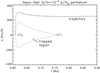 |
Fig. 2 Trajectory of the nanodust particle with Q∕m = 10−4 e/mp ejected fromthe comet (with orbital parameters of the comet Ikeya–Seki) at perihelium. The trajectory is shown in the (r, vr) plane. Also shown is the approximate trajectory obtained in the phase space model, and the separatrix trajectory which defines the boundary of the trapped region (the closed curve). The crosses show the positions of the fixed points of the phase space model. The outer fixed point is of the saddle point type, while the inner is a node, encircled by the trapped trajectories. |
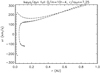 |
Fig. 3 Trajectories of the nanodust particles released from the orbit of the comet Ikeya–Seki before perihelium, at the heliocentric distances of 25 and 7 RS. The solid lines are the trajectories (projected onto the (r, vr) plane) obtained solving numerically the equations of motion for the nanodust particles with Q∕m = 10−4 e/mp, β = 0.1. The dashed lines are obtained from Eqs. (12) and (13). |
4 Motion of nanodust emitted from elongated orbits in the vicinity of the Sun
In this section, we present our results concerning the dynamics of nanodust particles emitted (at zero relative speed) from the parent bodies moving in high-eccentricity Keplerian orbits. We use the phase space model described in Sect. 4, as well as numerical solutions of the equation of motion for charged nanodust particles (Eq. (1)), with the solar wind and magnetic field described in Sect. 3.
4.1 Trapping conditions
Instead of analyzing the motion in the (r, v) phase plane, one can use the conservation law (Eq. (16)). The character of the particle motion (trapped or escaping) can be seen to depend on the initial conditions, which determine the coefficients of U(r).
The function U(r), which appears in the constant of motion (Eqs. (16) and (17)), is similar to the effectivepotential for the case of a particle interacting with a central force. In the present case, the force has both the attractive (the gravity) and the repulsive (the “centrifugal force”) components. The ~ 1∕r2 term, which dominates at small distances, is analogous to the angular momentum term. Depending on the coefficients of the respective terms, the function U(r) may have none or two extrema. In the latter case, there is a local minimum (a potential well) and a local maximum (the barrier) at the positions of the inner ( ) and the outer (
 ) root of W(r) = 0, respectively. The conditions for trapping are as follows:
- (1)
The initial position of the particle (at the heliocentric distance r0) must be inside the potential well:
 (19)
(19)
- (2)
The value of E must be smaller than the height of the barrier
 (the value of U(r) at the local maximum):
 (20)
(20)
In Eq. (20), v0 denotes the initial value of the radial component of the guiding center velocity. The coefficient of the 1∕r2 term in U(r) can be expressed in terms of the initial conditions for the nanodust particle at the point of release from the parent body
 (21)
(21)
where  is the initial tranverse speed of the particle in the plasma frame. The 1∕r2 term, which is the only one depending on initial velocity and therefore on the type of the orbit of the parent body, plays the role of the “repulsive core” in U(r). If its coefficient is too large, the potential well in U(r) becomes too shallow for trapping or vanishes altogether. This is the reason why trapping is disfavored for the case of nanodust released from the parent bodies moving at high transverse velocity, like the comets near perihelium.
In our model, the magnetic field B has no component along êθ. The transverse velocity vT of a particle can be written as  , where
  is the vector perpendicular to
  in the (êr, êϕ) plane. The transverse part of the plasma velocity has only the component along
  :
:
 (22)
(22)
The initial transverse velocity squared in the plasma frame at the point of release is therefore 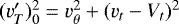 . If r0 is of the order 0.1 AU, then, near the solar equator (sinθ ≈ 1), Vt is comparable to the velocity for the circular Keplerian orbit. The initial velocity of the nanodust particle released from the larger body in the circumsolar cloud can be of the same order. In
  , Vt is subtracted from the
  component of the velocity of the nanodust particle, so that
  may becomesmall compared to GMS∕r0, provided that vθ is small. This partial cancellation can favor trapping for the particles released from the orbits with low inclination, or generally from the points on the orbit where the θ component of the orbital velocity is small.
A general expression for the transverse speed squared  along a planar trajectory can be written as
![Mathematical equation: \begin{eqnarray*} (v'_T)^2&=&v^2_{\chi}\frac{\sin^2i\ \sin^2\chi}{1-\sin^2i\ \cos^2\chi} \nonumber \\ && + \frac{1}{1+a^2}\left[a(v_r-V(r))+v_{\chi} \frac{\cos\ i}{(1-\sin^2i\ \cos^2\chi)^{1/2}}\right]^2\!,\end{eqnarray*}](/articles/aa/full_html/2018/09/aa32922-18/aa32922-18-eq62.png) (23)
(23)
where a = (Ω∕V (r))r sinθ (Eq. (8)), i is the inclination of the orbital plane in the heliographic coordinate system, vr = ṙ,  are the radial and azimuthal components of the velocity, and χ is the azimuthal angle in the plane of the orbit counted in the direction of motion, starting from the point where the orbit crosses the plane defined by the angular momentum vector and the solar rotation axis (if the point χ = 0 would correspond to the perihelium, χ would be the true anomaly). The heliographic co-latitude θ along the orbit can be expressed as cos θ = −sin icos χ. In the special case of i = 0,
![Mathematical equation: \begin{equation*} (v'_T)^2=\frac{1}{1+a^2}[a(v_r-V(r))+v_{\chi}]^2,\end{equation*}](/articles/aa/full_html/2018/09/aa32922-18/aa32922-18-eq64.png) (24)
(24)
with sinθ = 1, and for i = π∕2,
![Mathematical equation: \begin{equation*} (v'_T)^2=v^2_{\chi}+\frac{1}{1+a^2}[a(v_r-V(r))]^2,\end{equation*}](/articles/aa/full_html/2018/09/aa32922-18/aa32922-18-eq65.png) (25)
(25)
with sin θ = |sin χ|.
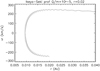 |
Fig. 4 Trajectories in the (r, vr) plane of the nanodust particle in the models with constant (model 1) and r-dependent (model 2) solar wind speed obtained by numerical solution of the equation of motion. The particle with Q∕m = 10−5 e/mp is emitted from the inbound part of the orbit of the comet Ikeya–Seki at initial heliocentric distance of 0.02 AU. The r-dependent solar wind case corresponds to a slight outward shift in the perihelium distance. |
4.2 Trapping of the nanodust emitted near the perihelion or aphelion
The initial value v0 of the radial component of the guiding center velocity as used in the phase space model is not identical with the initial radial velocity of the emitted particle. Instead, v0 is equal to the radial component of the sum of the initial parallel velocity of the particle v||,0 and the transverse plasma velocity VT at the point of release r0:
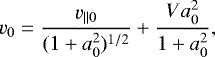 (26)
(26)
where a0 ≡ a(r0).
For a particle emitted near the perihelium or aphelium of the parent body orbit, we can nevertheless use v0 = 0 as a good approximation provided that a0 ≪ 1. The trapping condition (Eq. (20)) simplifies to
 (27)
(27)
In the region of r where  we can use an approximateexpression for U(r),
 (28)
(28)
After factoring out  , the trapping condition at the perihelium or aphelium can be written as
 (29)
(29)
where  , vorb (r0) = GMS∕r0 is the Keplerian velocity of a circular orbit at r0, and the function f is defined by
 (30)
(30)
We note that  , and that
  is required for trapping. At r0 ∕r1 → 0, the trapping condition Eq. (29) becomes α < 2(1 − β). Since df∕dx < 0, finite
  imply a still stricter upper limit.
For an elliptic orbit, the speed at the perihelium vper and aphelium vaph can be expressed in terms of the orbital eccentricity ϵ,
 (31)
(31)
where vorb(rper), vorb (raph) are the orbital speeds for the circular Keplerian orbit at the perihelium and aphelium distances, respectively. With the help of Eq. (23), and the relation  following from the definition of r1, we then obtain the expression for α at the perihelium and aphelium of an elliptic orbit. If the argument of the perihelium is equal to 90°,
![Mathematical equation: \begin{equation*} \alpha= \frac{1}{1+a^2}\left[-\left(\frac{r_0}{r_1}\right)^{3/2}(1-\beta)^{1/2} +(1\pm \epsilon)^{1/2}\frac{\cos i}{|\cos i|}\right]^2\!,\end{equation*}](/articles/aa/full_html/2018/09/aa32922-18/aa32922-18-eq79.png) (32)
(32)
and if it is equal to 0°,
![Mathematical equation: \begin{eqnarray*} \alpha&=&(1\pm \epsilon) \sin^2 i \nonumber \\* &&+\frac{1}{1+a^2}\left[-\left(\frac{r_0}{r_1}\right)^{3/2}(1-\beta)^{1/2} +(1\pm \epsilon)^{1/2}\cos i \right]^2\!.\end{eqnarray*}](/articles/aa/full_html/2018/09/aa32922-18/aa32922-18-eq80.png) (33)
(33)
The upper (lower) sign of ϵ applies for the perihelium (aphelium), respectively. We note that cos i∕|cosi| is + 1 for the inclination i < 90° (which corresponds to the prograde motion) and − 1 for i > 90° (the retrograde motion).
From Eqs. (32) and (33), it follows that if r0 ∕r1 ≪ 1 (which also implies a2 ≪ 1), then α ≈ 1 ± ϵ. The trapping condition at r0∕r1 → 0 becomes 1 + ϵ < 2(1 − β) at the perihelium, that is, ϵ < 0.8 at β = 0.1. This agrees with Figs. 5 and 6. The eccentricity values of the orbits of sungrazing comets are higher than 0.8, and therefore not consistent with trapping.
Figures 5 and 6 show the upper limits on the eccentricity of the parent body orbit consistent with trapping, obtained using the full expression for W(r), without the simplifying assumptionsv0 = 0,  1, r0 ∕r1 ≪ 1. The nanodust particle is released at the heliocentric distance r0 at zero velocity relative to the parent body. The initial radial velocity of the guiding center is given by Eq. (26). The release occurs at the perihelium of the parent body. The initial velocity of the guiding center in the (r, v) plane is obtained as the radial projection of the parallel velocity of the nanodust and the transverse velocity of the plasma.
Figure 5 illustrates the case where the orbits of the parent bodies have orientations corresponding to vθ = 0 at the perihelium (the argument of perihelium equal to 90° in heliographic coordinates). The two curves correspond to two different inclinations of the parent body orbits: 20° (the perihelium situated at heliographic co-latitude θ = 70°) and 70° (the perihelium at θ = 20°). The higher inclination of the parent body orbit corresponds in this case to a larger size (larger extension in r0) of the trapping region, with maximum r0 close to r1 for the appropriate value of θ. This agrees with the results for circular orbits obtained by Czechowski & Mann (2010, 2012). The broad peaks near the outer limits in r0 are due to the reduction of initial  of the emitted particle by taking account of the plasma motion (the
  term in Eq. (32)). Also shown are the results from full numerical simulations of the nanodust motion (asterisks for θ = 70° and diamonds for θ = 20°). We note the effect of including the Poynting–Robertson force in the full simulation (the asterisks linked by the dotted line). The contraction of the particle orbit by the Poynting–Robertson force relaxes the upper limit on the initial velocity of the trapped particle.
Figure 6 presents the results for the case where the argument of perihelium is equal to 0° in heliographic coordinates (the point of perihelium lies in the solar equator plane). The curves labelled 1–7 correspond to different values of inclinations of the parent body orbit, from 0° to 180°. At intermediate inclinations, the initial velocity of the emitted particle is not parallel to the solar equator plane (the component along êθ direction is not zero). The effect of orbital inclination on the size of the trapped region is opposite to that seen inFig. 5: higher inclination corresponds to a trapped region more restricted in r0, again in agreement with the result of Czechowski & Mann (2010, 2012) for circular orbits. The trapping can be seen to become more difficult when the initial orbital velocity departs from the prograde direction, because the two terms in the square brackets in Eq. (33), corresponding to transverse components of the plasma and orbital velocity, have the same sign and so cannot (partly) cancel each other.
Figure 6 also illustrates the effect of drag force on trapping. In particular, for model 2 of the solar wind, the effect of Poynting–Robertson drag alone (squares) can be seen to be much weaker than the combination of Poynting–Robertson and the proton drag (X signs). We also note that the drag relaxes the upper limit on eccentricity by a large amount (from ~0.53 at r0 = 0.11 AU to ~0.73 at r0 ≈ 0.15 AU), while the outer limit in r of the trapped region is increased only slightly. The effect of the proton drag is strong because model 2 corresponds to high plasma density in the vicinity of the Sun.
If the particle is emitted from the aphelium of the orbit, the initial velocity of the particle is less than the Keplerian velocity of the circular orbit. If the aphelium distance is within the trapping region ( ), trapping may be possible for any eccentricity. However, when the point of release r0 approaches the outer limit of the trapping region, the limits on eccentricity do appear (see Fig. 7).
The cases shown in Fig. 7 correspond to hypothetical bodies in high-eccentricity orbits with aphelium distances well within 1 AU of the Sun. We include this figure to highlight the difference between the trapping-induced constraints on eccentricity for prograde and retrograde orbits. For prograde orbits with the argument of the perihelium equal to 90°, the trapping region extends to r = r1 thanks to partial cancellation (possible up to some upper limit in eccentricity) between the orbital speed at aphelium and the transverse component of the solar wind speed. For retrograde orbits, this cancellation is not possible, because both terms have the same sign. In this case, trapping of nanodust is only possible when a parent body at aphelium is travelling at low orbital speeds, which puts a lower limit on the orbital eccentricity.
For the orbits typical of the comets, the aphelium distances are beyond the outer limit of the trapping region. The exception is the case of the orbit with the aphelium point situated very close to the solar rotation axis. Since r1 behaves as  with the heliographic co-latitude θ, the distance to the boundary of the trapping region in our model increases with decreasing θ. At the same time, the width inθ of the trapping region contracts, so that at 1.6 AU the region is already restricted to directions less than 2° away from the solar rotation axis.
Trapping of nanodust emitted near the apoapsis of a comet may be a realistic possibility for the stars with rotation speeds much lower than the solar value.
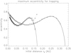 |
Fig. 5 Upper limit on the eccentricity of the orbit of the parent body consistent with trapping of the nanodust particle emitted at zero relative speed at the perihelium (heliocentric distance r0). The argument of the perihelium of the orbit is 90° in heliographic inertial coordinates, so that the initial velocity of the particle is parallel to solar equator (vθ = 0). The solid lines are derived from the phase space model (Eqs. (19) and (20)). The symbols show the results from numerical simulations (Eq. (1)). The two sets of curves correspond to different heliolatitudes of the point of release: colatitude θ = 70° (asterisks) and 20° (diamonds), respectively. The asterisks linked by the dotted line show the result (for θ = 70°) from the simulation including the Poynting–Robertson force. |
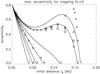 |
Fig. 6 As in Fig. 5, but the argument of perihelium of the parent body orbit is 0° in heliographic coordinates (the point of perihelium lies in the solar equator plane). The cases illustrated correspondto different inclinations of the parent body orbits. The numbers 1–7 mark the inclinations 0°, 20°, 50°, 70°, 85°, 110°, and 180°, respectively. Also shown are the results from numerical solutions to the full equations of motion for Q∕m = 10−4 e/mp grains. The cases shown are constant speed SW, no PR drag (diamonds); the same with PR drag included (triangles); distance-dependent SW speed (model 2) with PR drag included (squares); model 2 with both PR and the proton drag (× symbols). |
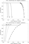 |
Fig. 7 Limits on eccentricity of the parent body orbit imposed by trapping of nanodust emitted from the aphelium of the orbit. The argument of perihelium is 90°. Eight values of orbital inclinations are considered: four prograde: 0°, 50°, 70°, and 85° (upper panel) and four retrograde: 95°, 110°, 130°, and 180° (lower panel). When the nanodust is emitted near to the (inclination-dependent) outer limit of the trapping region, the trapping requirement limits the eccentricity of the orbit from above (the prograde orbit, upper panel, solid lines) or from below (the retrograde orbit, lower panel, dashed lines). For retrograde orbits, the trapping region is less extended than for prograde ones. Also shown are results from numerical simulations (slow wind only) for the grains with Q∕m = 10−4 e/mp (diamonds) and Q∕m = 3 × 10⁻⁴ e/mp (squares). In these cases the PR drag has no appreciable effect on results. In the prograde case, the value of Q∕m had to be raised to 3 × 10⁻⁴ e/mp to obtain a good agreement with the phase space model. |
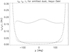 |
Fig. 8 Extent of the potential well of the effective potential U(r) for particles emitted at different points along the orbit of the comet Ikeya–Seki, parametrized by the angle χ counted from the perihelium. The upper (lower) half of the dotted oval shows the value of |


4.3 Nanodust emitted from an arbitrary point along the orbit
In this subsection, we use three high-eccentricity orbits as examples, chosen to be representative of fragments of the comet Ikeya–Seki and of two classes of meteoroids: the Aquarids and the Geminids, associated with a comet and an asteroid, respectively. Because the angle between the solar equator plane and the ecliptic plane is small, for simplicity we use the orbital parameters given in the ecliptic coordinates without changing our solar inertial system. The assumed orbital parameters are listed in Table 1.
Although none of the nanodust particles released from these orbits are trapped, the parameters of the phase space model are still relevant for their dynamics. We find that the real zeroes of the function W(r) and therefore the “potential well” are typically present only for parts of the orbit. The existence of the “potential well” affects the motion of nanodust particles even in the absence of trapping, and, in the case of  , opens a “corridor” permitting charged nanodust particles to approach very close to the Sun.
Figures 8, 9, and 11 show the values of  and
and  along the orbits listed in Table 1. Figure 10 shows the velocity distribution along two of theseorbits. We also include the hypothetical case of the orbit with the inclination and perihelium as for Aquarids, but with the eccentricity reduced to 0.4. The orbits are parameterized by the azimuthal angle χ. The dotted ovals show the values of
  (upper line) and
  (lower line). In the first two cases, there are regions of χ where
  and
and  are not defined. In the third case,
  and
and  are defined over the whole of the orbit. The zeros
  and
and  appear and vanish as a pair. Trapping of the nanodust occurs only in the case of the orbit with reduced eccentricity, with the trapped region occupying only a fraction of the region where
  and
and  are defined.
In addition to the orbits listed in Table 1, we have checked the trapping conditions for a sample of 270 000 orbits. The sample was divided into ten eccentricity classes with eccentricities 0.0, 0.2, 0.5, 0.6, 0.7, 0.8,0.87, 0.9, and 0.97. Within each class, the orbital parameters each spanned 30 values of the perihelium distance rmin (logarithmic distribution between 0.008 and 0.5 AU), the orbital inclination i (uniform distribution between 0° and 180°) and the parameter of the perihelium ϕc (uniform distribution between 0° and 360°). The right ascension was taken the same for all orbits. The trapping condition was checked along each orbit at 100 points with equal separation in the azimuthal angle.
Figure 12 shows the resulting distributions, over the azimuthal angle, of the points for which the trapping condition is satisfied. We did not attempt to use realistic weight factors: the distributions were obtained assuming that each orbit in the sample has the same weight. The results are shown for four classes of the orbits, defined by the requirement that the eccentricity of the orbit must exceed a given minimum value: 0.4, 0.6, 0.8, and 0.87. For increasing eccentricity, the trapped region along the orbit becomes restricted to the vicinity of the aphelium. For the case of eccentricity above 0.87, Fig. 12 shows that trapping may occur only for the points more than ±90° away from the perihelium.
The effective potential can also be used to find the minimum heliocentric distance which the nanodust particle reaches after release from the parent body. Figures 13–15 show the results for the nanodust released from the orbits of Ikeya–Seki, the Aquarids, and the Geminids, respectively. The results obtained from the phase space model (the solid line) agree with the results of full numerical solution (the diamonds) for the Q∕m = 10−4 e/mp nanodust, with one exception caused by the encounter with the current sheet.
The nanodust released from the inbound part of the orbit comes closer to the Sun than the parent body does. For the orbits of Aquarids (Fig. 14) and of Geminids (Fig. 15), this effect is particularly strong: the nanodust released within a certain sector of the parent body orbit can, thanks to electromagnetic forces, approach the Sun to within a much shorter distance (here by an order of magnitude) than the orbital perihelium. We call this phenomenon a “corridor to the Sun”. We also note that the points of minimum heliocentric distances reached by the nanodust occur near the points of minimum  (compare with Fig. 9).
Assumed orbital parameters.
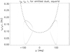 |
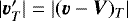
Fig. 9 As in Fig. 8 but for the orbit of Aquarids. In this case the extrema of the potential U(r) exist within two separate regions (the dotted ovals). |
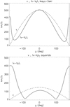 |
Fig. 10 Orbital speed |v| and the transverse speed relative to solar wind plasma |


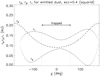 |
Fig. 11 As in Fig. 9 but for the orbit of a hypothetical body with the same inclinationand perihelium as for Aquarids, but with the eccentricity reduced to a smaller value (0.4). In this case there exists a trapping region for emitted nanodust, with the limits in χ shown by the vertical dotted lines. |
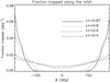 |
Fig. 12 Distributions (over the azimuthal angle ϕ counted from the perihelium) of the points at which the trapping condition is satisfied, calculated for a large sample of hypothetical parent body orbits with different parameters (see the text). The curves shown correspond to the orbits with the eccentricities ϵ ≥ 0.87, 0.8, 0.6, and 0.4, respectively. The distributions are normalized so that the integral over ϕ is equal to 1. |
4.4 Propagation to 1 AU
Ultimately, the nanodust particles emitted from high-eccentricity orbits escape away from the Sun. Figure 16 shows the trajectories of a sample of grains emitted from the orbit of the comet Ikeya–Seki, projected onto the heliographic longitude–latitude plane. All trajectories end at 1 AU from the Sun. The small particles (Q∕m = 10−4 e/mp) stay close to the constant heliolatitude cones (θ = const.), meaning that their motion projected onto the sky is directed along the heliographic parallel. For Q∕m = 10−5 e/mp particles, the motion includes a significant amount of drift. As expected, the drift direction depends on the magnetic field polarity. Our simulations are restricted to the case of defocusing magnetic field, so that the drift of positively charged particles is directed away from the heliospheric current sheet. To imitate the focusing polarity, we also include results of simulations for particles with negative charges. In particular, the drift of particles with Q∕m = –10−6 e/mp enables them to encounter the current sheet and commence drifting along its surface (see Fig. 16).
The speed of nanodust particles as a function of distance is illustrated in Fig. 17. The particles emitted from the inbound part of the orbit initially approach the Sun with a substantial velocity gain, as predicted by the phase space model. After passing the point of minimum heliocentric distance, their velocity first decreases and then, for the case of small particles (Q∕m = 10−4 and 10−5 e/mp), increases again, reaching, at 1 AU, the value close to the velocity of the solar wind. For particles with Q∕m = 10−6 and 10−7 e/mp, the asymptotic speed is much lower (Fig. 17, bottom panel). The asymptotic speeds are similar to those obtained in (Czechowski & Mann 2010, 2012) for particles emitted from circular orbits (see also Juhasz & Horanyi 2013).
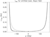 |
Fig. 13 Minimum heliocentric distance rmin (solid line)reached by nanodust particles emitted from the comet Ikeya–Seki as a function of the parameter χ (angle counted from the perihelium) of the release point on the orbit of the comet. The orbit of the comet is shown by the dashed line, describing also the initial points of the nanodusttrajectories. The diamonds show the results from full numerical simulations for Q∕m = 10−4 e/mp. |
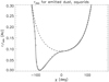 |
Fig. 14 As in Fig. 13 but for the orbit of Aquarids. In this case there is a “corridor to the Sun”, a range of initial points inside 0.25 AU on the inbound part of the orbit for which the dust particles can approach the Sun much closer than the parent body. |
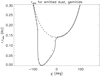 |
Fig. 15 As in Fig. 13 but for the orbit of Geminids. In this case also a “corridor” forms, for which the dust particles can approach the Sun much closer than the parent body. We note the large disagreement between the phase space model(solid line) and full simulation for one data point. This is caused by the encounter of the nanodust particle soon after emission with the heliospheric current sheet (the phase space model does not include the current sheet). |
4.5 Effect of the proton drag force
The proton drag force becomes important only for trajectories that pass through a region with a very high proton density, within a few solar radii from the surface of the Sun. The effect depends on the assumed model of the solar wind. A nanodust particle approaching very close to the Sun becomes reflected by the magnetic mirror force. In the absence of drag, the reflection process is approximately symmetric in time: the particle emerges with the same speed as it had before the reflection. The drag force causes the particle to slow down, breaking the symmetry (Fig. 18).
For the case of trapped nanodust studied in Czechowski & Kleimann (2017), the particles return repeatedly to the vicinity of the Sun andthe effect of drag is cumulative, leading to contraction of the orbit and ultimate destruction of the particle. According to present simulations, the nanodust particles emitted from high-eccentricity orbits do not approach close to the Sun more than once. As a consequence, the total effect of drag is not strong enough to prevent the particles from escaping from the Sun into the region where the drag becomes irrelevant compared to other forces.
In Fig. 18 we compare the effect of proton drag for different models of the solar wind. As expected, the strongest effect is obtained for the models with high values of the proton density in the vicinity of the Sun (models 2 and 3; see Fig. 1).
4.6 Effects of sublimation
In the vicinity of the Sun, the destruction of nanodust by sublimation and sputtering becomes an important problem. This requires a dedicated study, and is beyond the scope of this work. However, we present here some estimations based on the results obtained forthe case of the dust in slowly evolving orbits (Krivov et al. 1998). The study we refer to was based on assuming large (micrometer-sized) carbon and silicate particles at equilibrium temperature where absorbed and emitted radiation are balanced.
For dustin the nm size range, the number of absorbed photons can be small and absorption rate stochastic. According to Li & Mann (2012), at the distances less than ~1 AU from the Sun, the phenomenon of temperature spikes and general stochastic heating will not occur for the grain sizes above 1 nm. Our estimation (see Czechowski & Mann 2010) of the radius of a nanodust particle with Q∕m = 10−5 e/mp (Q∕m = 10−4 e/mp) is 10 nm (3 nm). We, therefore, shall not consider stochastic heating.
Krivov et al. (1998) have shown that fast sublimation of the dust commences at the heliocentric distance of ~3 RSun, with the lifetime of the 0.1 μm grain equal to 0.01 yr. Following Krivov et al. (1998), we assume that, inside the fast sublimation region, the sublimation lifetime is proportional to the grain radius. The lifetime of a 10 nm (3 nm) grain is then 0.001 yr (0.0003 yr), that is, 0.365 (0.109) days. The time needed to sublimate a 1 nm thick layer is 0.036 days.
We can use the results of our trajectory calculations to find how much time a particle spends inside the fast-sublimation region, defined by the condition that the heliocentric distance is less than 3 RSun. Comparing this time with the sublimation time taken from Krivov et al. (1998), we can calculate whether or not the particle is likely to survive.
We note, however, that the results of Krivov et al. (1998) were not derived for the case of grains with large radial velocities, which is a frequent case in our trajectories. Using their result is approximately equivalent to assuming the sublimation rate valid at r ~ 3RSun. Since the sublimation rate is likely to increase towards the Sun, we expect that our results underestimate the effect of sublimation.
We now consider the nanodust trajectories used in Figs. 13–15, corresponding to nanodust emitted from the orbit of the comet Ikeya–Seki, the Aquarids and the Geminids, respectively. The diamonds show the points of closest approach to the Sun for these trajectories.
For the case of Aquarids (Fig. 14) and Geminids (Fig. 15), only the trajectories near the tip of the “corridor” (5 points with χ = –79° to –94° for Fig. 14 and 4 points with χ = –51° to –73° for Fig. 15) enter the fast sublimation region. The time tin spent inside the fast-sublimation region is almost exactly the same for the trajectories of Q∕m = 10−4 e/mp and Q∕m = 10−5 e/mp nanodust. tin varies between 0.13 and 0.16 days, the only exception being one point in Fig. 14 (χ = –94°), where tin = 0.08 days. Apart from this exception, the tin values are high enough for destruction of particles with radii of 3 nm. The nanodust with the radius 10 nm would be destroyed only if the sublimation rate inside 3RSun were significantly higher than implied by the results of Krivov et al. (1998).
The perihelion of the comet Ikeya–Seki (Fig. 13) lies inside the fast sublimation zone. The trajectories entering the fast sublimation region correspond to the dust emitted from the points between χ = –133° and χ = 56° along the orbit. The values of tin vary from 0.034 to 0.089 days for most of this interval. Only for χ = –128° to –103° is tin between 0.113 and 0.130 days, above the sublimation lifetime of the 3 nm nanodust. We conclude that the 3 nm nanodust may in some cases avoid destruction, even if emitted inside the fast sublimation zone.
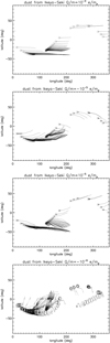 |
Fig. 16 Heliographic longitude–latitude projection of the sample of trajectories of nanodust emitted from the orbit of the comet Ikeya–Seki. The trajectories end at 1 AU from the Sun. The points of emission are marked by squares. Separate panels show the results for nanodust with different Q∕m ratios. The cases of positive charge: Q∕m = 10−4 e/mp and Q∕m = 10−5 e/mp show the behavior of nanodust for the “defocusing” solar magnetic field polarity. The results for nanodust with Q∕m set to negative values: Q∕m = –10−5 e/mp and Q∕m = –10−6 e/mp represent also the behavior of the positively charged dust for the “focusing” polarity. For the Q∕m = –10−6 e/mp case, the drift along the heliospheric current sheet occurs for some trajectories. |
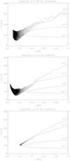 |
Fig. 17 Velocity as a function of heliocentric distance for nanodust grains with Q∕m = 10−4, 10−5, 10−6, and 10−7 e/mp emitted from the orbit of Aquarids at the perihelium (0.09 AU from the Sun, the upper panel), and at the distance 0.2 AU on the inbound (middle panel) and outbound (lower panel) parts of the orbit. |
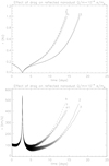 |
Fig. 18 Effect of proton drag on nanodust emitted from the inbound part of the orbit of Aquarids at the distance r = 0.17 AU from the Sun. The cases illustrated are (including the proton drag) (1) V = const. solar wind (model 1), (2) Sheeley et al. (1997) profile (model 2), and (3) modified V (r) profile (model 3). The results for the same solar wind models but with the proton drag neglected are marked (a), (b), and (c), respectively. |
5 Discussion and conclusions
The first application of our method of combining the phase space model (the early version) with the numerical simulations was to the case of nanodust produced by collisional fragmentation of larger particles in the circumsolar dust cloud (Czechowski & Mann 2010, 2012). In the present work, we consider the other possible source of dust, the cometary bodies, including the sungrazing comets and their remains. Specifically, we consider a sample of three orbits: the orbit of Aquarids, of Geminids, and, as an example of the Kreutz group, the orbit of the comet Ikeya–Seki. The orbits are in fact approximate, because, for simplicity, we use the orbital parameters given in ecliptic coordinates instead of transforming to heliographic inertial coordinates used in the present work.
The purely radial, time-stationary solar wind that our model describes is obviously only an approximation. However, in a recent study (Czechowski & Kleimann 2017) based on a numerical MHD model of the solar corona during a coronal mass ejection (CME), it was found that some predictions of our model remain valid. In particular, the trapped nanodust population predicted by Czechowski & Mann (2010, 2012) was found to appear and survive in the simulated CME. This result gives us hope that the simple description of a charged particle motion given by our phase space model can also be applied in more realistic situations.
The new version of our 2D phase space model used in the present work is applicable to the case of a distance-dependent solar wind speed. A somewhat unexpected prediction of the model is that the charged scatter-free particle motion in the vicinity of the Sun is largely independent of the solar wind speed profile. The applications of the new version of the model are helped by the fact that it has a constant of motion, given by a simple formula. As a result, we can now derive an analytical expression for the radial velocity component of a particle as a function of the heliocentric distance. The conservation law also provides a way to determine the turning points of the particle radial motion, and a test for whether or not the particle is trapped. For particles with high-enough charge-to-mass ratio (Q∕m = 10−5–10−4 e/mp) the results of the model agree well with the numerical solutions of full equations of motion.
Our main conclusion is that the mechanism of trapping the nanodust particles in nonKeplerian orbits in the vicinity of the Sun, which was derived (Czechowski & Mann 2010, 2012) for the nanodust created in the circumsolar cloud, is not effective for the case of nanodust particles emitted from highly eccentric orbits, like those of the comets. The nanodust coming from the comets would therefore not contribute to the (so far hypothetical) trapped dust population around the Sun.
Trapping becomes ineffective because the nanodust from the comets is created with high initial transverse velocity in the plasma frame. The trapping condition then implies an upper limit on the eccentricity of the orbit of the parent body. The limit depends on the orientation of the orbit and on the point at which the nanodust is released. Trapping may take place for eccentricity as high as 0.8 but only in the most favorable circumstances. Results of our previous works show that the trapping is typically even less likely when the dust has a nonzero initial velocity relative to the parent body, due, for example, to the acceleration in the coma. In a recent study, the acceleration of 1 to 10 nm sized nanodust near a comet was simulated (Gunell et al. 2015) within the coma. The calculations show that the nanodust resides in the coma for typically 1000–10 000 s. It is accelerated in the direction of the electric field and the final speed can range from several up to several tens of kilometres per second when it leaves the coma and emerges in the solar wind.
Even if it cannot be trapped, the nanodust released from the inbound part of a highly eccentric orbit may approach the Sun to within distances much closer than the perihelium of the parent body. The minimum distance is strongly dependent on the initial point on the parent body orbit (a “corridor” to the Sun). After reaching the minimum distance, the particle is reflected by the magnetic mirror force. All nanodust particles emitted from the parent body (except those destroyed by sublimation on the way) escape away from the Sun, reaching velocities of the order of ~400 km s−1 at 1 AU.
The drag force due to ion impacts on the grain (Minato et al. 2004) was found in Czechowski & Kleimann (2017) to have a significant effect on nanodust (particularly, the trapped component) in the solar corona. We therefore included, in part of our simulations, the proton drag force described by the same approximate expression as in Czechowski & Kleimann (2017), with the plasma parameters taken from our models (1–3). For particles bypassing the Sun by more than ~0.015 AU, we found drag to be unimportant. For a particle approaching even closer to the Sun (0.006 AU), the effect was still negligible for model 1 of the solar wind, but for models 2 and 3 (corresponding to a higher proton density in the solar corona), the effect of drag appeared as an approximately three-day delay in the escape time to 1 AU.
The above estimate may be only of academic interest because of high probability of destruction of nanodust particles passing very close to the Sun. The spectral slope of the F-corona brightness suggests that most of the dust sublimates at distances of about 0.02 AU (see Mann 1992). Based on temperature and sublimation calculations, different authors have predicted dust free zones ranging from 1.5 solar radii outward to 40 solar radii, depending on the dust materiel (summarized in Mann et al. 2004).
A detailed study of nanodust trajectories including the possibility of destruction is an interesting goal for future studies. Aside from the dust sublimation, sputtering (see, e.g., Ragot & Kahler 2003) and dust collisions (Czechowski & Mann 2010) also need to be taken into account.
In the present work, we restrict ourselves to a simplified approach. We combine our nanodust trajectory calculations with the sublimation lifetimes derived by Krivov et al. (1998) for the case of dust in slowly evolving orbits. Since we consider the particles sizes above 1 nm in the vicinity of the Sun, we can neglect the possibility of stochastic heating (Li & Mann 2012).
For a sample of nanodust trajectories considered in this work, we find that the 10 nm particles which enter the sublimation zone along the “corridors” to the Sun are likely to survive, unless the sublimation rates for nanodust are significantly higher than those obtained by Krivov et al. (1998). The 3 nm particles in similar trajectories are destroyed. A result of some interest is the survival of particles (including the 3 nm ones) emitted inside the fast sublimation region from the outbound part of the orbit of the comet Ikeya–Seki.
Our simulations include propagation of nanodust to the maximum distance of 1 AU. Similar to the case of nanodust released from circular orbits (Czechowski & Mann 2010, 2012; Juhasz & Horanyi 2013), the results are sensitive to magnetic field polarity.
Acknowledgements
This work is supported by the Research Council of Norway (grant number 262941). We thank the anonymous reviewer for constructive comments.
References
- Bale, S. D., Goetz, K., & Harvey, P. R. et al., 2016, Space Sci. Rev., 204, 49 [NASA ADS] [CrossRef] [Google Scholar]
- Burch, J. L., Gombosi, T. I., Clark, G., Mokashi, P., & Goldstein, R. 2015, Geophys. Res. Lett., 42, 6575 [NASA ADS] [CrossRef] [Google Scholar]
- Czechowski, A., & Kleimann, J. 2017, Ann. Geophys., 5, 1033 [NASA ADS] [CrossRef] [Google Scholar]
- Czechowski, A., & Mann, I. 2010, ApJ, 714, 89 [NASA ADS] [CrossRef] [Google Scholar]
- Czechowski, A., & Mann, I. 2011, ApJ, 732, 127 [NASA ADS] [CrossRef] [Google Scholar]
- Czechowski, A., & Mann, I. 2012, in Nanodust in the Solar System: Discoveries and Interpretations, eds., I. Mann, N. Meyer-Vernet, & A. Czechowski (New York: Springer) [Google Scholar]
- Fox, N. J., Velli, M. C., Bale, S. D., et al. 2016, Space Sci. Rev., 204, 7 [NASA ADS] [CrossRef] [Google Scholar]
- Gombosi, T. I., Burch, J. L., & Horanyi, M. 2015, A&A, 583, A23 [NASA ADS] [CrossRef] [EDP Sciences] [Google Scholar]
- Gunell, H., Mann, I., Simon Wedlund C., et al. 2015, I Planet. Space Sci., 119, 1323 [Google Scholar]
- Juhasz, A., & Horanyi, M. 2013, Geophys. Res. Lett., 40, 2500 [NASA ADS] [CrossRef] [Google Scholar]
- Kellogg, P. J., Goetz, K., & Monson, S. J. 2016, J. Geophys. Res. Space Phys., 121, 966 [NASA ADS] [CrossRef] [Google Scholar]
- Kimura, H., & Mann, I. 1998, ApJ, 499, 454 [NASA ADS] [CrossRef] [Google Scholar]
- Krivov, A., Kimura, H., & Mann, I. 1998, Icarus, 134, 311 [NASA ADS] [CrossRef] [Google Scholar]
- Li, A., & Mann, I. 2012, Astrophys. Space Sci. Lib., 385, 5 [Google Scholar]
- Malaspina, D. M., Horanyi, M., Zaslavsky, A., et al. 2014, Geophys. Res. Lett., 41, 266 [NASA ADS] [CrossRef] [Google Scholar]
- Mann, I. 1992, A&A, 261, 329 [NASA ADS] [Google Scholar]
- Mann, I. 2017, Phil. Trans. Royal Soc. A, 375, 2097 [Google Scholar]
- Mann, I., & Czechowski, A. 2005, ApJ, 624, L125 [NASA ADS] [CrossRef] [Google Scholar]
- Mann, I., Kimura, H., Biesecker, D. A., et al. 2004, Space Sci. Rev., 110, 269 [NASA ADS] [CrossRef] [Google Scholar]
- Mann, I., Murad, E., & Czechowski, A. 2007, Planet. Space Sci., 55, 1000 [NASA ADS] [CrossRef] [Google Scholar]
- Mann, I., Meyer-Vernet, N., Czechowski, A. 2014, Phys. Rep., 536, 1 [NASA ADS] [CrossRef] [Google Scholar]
- Meyer-Vernet, N., Maksimovic, M., Czechowski, A., et al. 2009, Sol. Phys., 256, 463 [NASA ADS] [CrossRef] [Google Scholar]
- Minato, T., Köhler, M., Kimura, H., et al. 2004, A&A, 424, L13 [NASA ADS] [CrossRef] [EDP Sciences] [Google Scholar]
- Mukai, T. 1981, A&A, 99, 1 [NASA ADS] [Google Scholar]
- Mueller, D., Marsden, R. G., St. Cyr, O. C., et al. 2013, Sol. Phys., 285, 25 [NASA ADS] [CrossRef] [Google Scholar]
- Northrop, T. G. 1958, Adiabatic Motion of Charged Particles (New York: John Wiley & Sons, Inc.) [Google Scholar]
- Ragot, B. R., Kahler, S. W. 2003, ApJ, 594, 1049 [NASA ADS] [CrossRef] [Google Scholar]
- Sheeley, N. R., Wang, Y.-M., Hawley, S. H., et al. 1997, ApJ, 484, 472 [NASA ADS] [CrossRef] [Google Scholar]
- Snios, B., Lewkow, N., & Kharchenko, V. 2014, A&A, 568, A80 [NASA ADS] [CrossRef] [EDP Sciences] [Google Scholar]
- Szego, K., Juhasz, A., & Bebesi, Z. 2014, Planet. Space Sci., 99, 48 [NASA ADS] [CrossRef] [Google Scholar]
- Utterback, N. G., & Kissel, J. 1990, AJ, 100, 1315 [NASA ADS] [CrossRef] [Google Scholar]
- Utterback, M. G., & Kissel, J. 1995, Astrophys. Space Sci., 225, 327 [NASA ADS] [CrossRef] [Google Scholar]
All Tables
All Figures
|
Fig. 1 Solar wind speed (upper panel) and the proton density (bottom panel) profiles used in our simulations (the slow wind component). The models 1, 2, and 3 are presented by the dotted, solid, and dashed lines, respectively. For the fast wind, the speed should be multiplied by 2, and the density divided by 4. |
| In the text | |
|
Fig. 2 Trajectory of the nanodust particle with Q∕m = 10−4 e/mp ejected fromthe comet (with orbital parameters of the comet Ikeya–Seki) at perihelium. The trajectory is shown in the (r, vr) plane. Also shown is the approximate trajectory obtained in the phase space model, and the separatrix trajectory which defines the boundary of the trapped region (the closed curve). The crosses show the positions of the fixed points of the phase space model. The outer fixed point is of the saddle point type, while the inner is a node, encircled by the trapped trajectories. |
| In the text | |
|
Fig. 3 Trajectories of the nanodust particles released from the orbit of the comet Ikeya–Seki before perihelium, at the heliocentric distances of 25 and 7 RS. The solid lines are the trajectories (projected onto the (r, vr) plane) obtained solving numerically the equations of motion for the nanodust particles with Q∕m = 10−4 e/mp, β = 0.1. The dashed lines are obtained from Eqs. (12) and (13). |
| In the text | |
|
Fig. 4 Trajectories in the (r, vr) plane of the nanodust particle in the models with constant (model 1) and r-dependent (model 2) solar wind speed obtained by numerical solution of the equation of motion. The particle with Q∕m = 10−5 e/mp is emitted from the inbound part of the orbit of the comet Ikeya–Seki at initial heliocentric distance of 0.02 AU. The r-dependent solar wind case corresponds to a slight outward shift in the perihelium distance. |
| In the text | |
|
Fig. 5 Upper limit on the eccentricity of the orbit of the parent body consistent with trapping of the nanodust particle emitted at zero relative speed at the perihelium (heliocentric distance r0). The argument of the perihelium of the orbit is 90° in heliographic inertial coordinates, so that the initial velocity of the particle is parallel to solar equator (vθ = 0). The solid lines are derived from the phase space model (Eqs. (19) and (20)). The symbols show the results from numerical simulations (Eq. (1)). The two sets of curves correspond to different heliolatitudes of the point of release: colatitude θ = 70° (asterisks) and 20° (diamonds), respectively. The asterisks linked by the dotted line show the result (for θ = 70°) from the simulation including the Poynting–Robertson force. |
| In the text | |
|
Fig. 6 As in Fig. 5, but the argument of perihelium of the parent body orbit is 0° in heliographic coordinates (the point of perihelium lies in the solar equator plane). The cases illustrated correspondto different inclinations of the parent body orbits. The numbers 1–7 mark the inclinations 0°, 20°, 50°, 70°, 85°, 110°, and 180°, respectively. Also shown are the results from numerical solutions to the full equations of motion for Q∕m = 10−4 e/mp grains. The cases shown are constant speed SW, no PR drag (diamonds); the same with PR drag included (triangles); distance-dependent SW speed (model 2) with PR drag included (squares); model 2 with both PR and the proton drag (× symbols). |
| In the text | |
|
Fig. 7 Limits on eccentricity of the parent body orbit imposed by trapping of nanodust emitted from the aphelium of the orbit. The argument of perihelium is 90°. Eight values of orbital inclinations are considered: four prograde: 0°, 50°, 70°, and 85° (upper panel) and four retrograde: 95°, 110°, 130°, and 180° (lower panel). When the nanodust is emitted near to the (inclination-dependent) outer limit of the trapping region, the trapping requirement limits the eccentricity of the orbit from above (the prograde orbit, upper panel, solid lines) or from below (the retrograde orbit, lower panel, dashed lines). For retrograde orbits, the trapping region is less extended than for prograde ones. Also shown are results from numerical simulations (slow wind only) for the grains with Q∕m = 10−4 e/mp (diamonds) and Q∕m = 3 × 10⁻⁴ e/mp (squares). In these cases the PR drag has no appreciable effect on results. In the prograde case, the value of Q∕m had to be raised to 3 × 10⁻⁴ e/mp to obtain a good agreement with the phase space model. |
| In the text | |
|
Fig. 8 Extent of the potential well of the effective potential U(r) for particles emitted at different points along the orbit of the comet Ikeya–Seki, parametrized by the angle χ counted from the perihelium. The upper (lower) half of the dotted oval shows the value of |
| In the text | |
|
Fig. 9 As in Fig. 8 but for the orbit of Aquarids. In this case the extrema of the potential U(r) exist within two separate regions (the dotted ovals). |
| In the text | |
|
Fig. 10 Orbital speed |v| and the transverse speed relative to solar wind plasma |
| In the text | |
|
Fig. 11 As in Fig. 9 but for the orbit of a hypothetical body with the same inclinationand perihelium as for Aquarids, but with the eccentricity reduced to a smaller value (0.4). In this case there exists a trapping region for emitted nanodust, with the limits in χ shown by the vertical dotted lines. |
| In the text | |
|
Fig. 12 Distributions (over the azimuthal angle ϕ counted from the perihelium) of the points at which the trapping condition is satisfied, calculated for a large sample of hypothetical parent body orbits with different parameters (see the text). The curves shown correspond to the orbits with the eccentricities ϵ ≥ 0.87, 0.8, 0.6, and 0.4, respectively. The distributions are normalized so that the integral over ϕ is equal to 1. |
| In the text | |
|
Fig. 13 Minimum heliocentric distance rmin (solid line)reached by nanodust particles emitted from the comet Ikeya–Seki as a function of the parameter χ (angle counted from the perihelium) of the release point on the orbit of the comet. The orbit of the comet is shown by the dashed line, describing also the initial points of the nanodusttrajectories. The diamonds show the results from full numerical simulations for Q∕m = 10−4 e/mp. |
| In the text | |
|
Fig. 14 As in Fig. 13 but for the orbit of Aquarids. In this case there is a “corridor to the Sun”, a range of initial points inside 0.25 AU on the inbound part of the orbit for which the dust particles can approach the Sun much closer than the parent body. |
| In the text | |
|
Fig. 15 As in Fig. 13 but for the orbit of Geminids. In this case also a “corridor” forms, for which the dust particles can approach the Sun much closer than the parent body. We note the large disagreement between the phase space model(solid line) and full simulation for one data point. This is caused by the encounter of the nanodust particle soon after emission with the heliospheric current sheet (the phase space model does not include the current sheet). |
| In the text | |
|
Fig. 16 Heliographic longitude–latitude projection of the sample of trajectories of nanodust emitted from the orbit of the comet Ikeya–Seki. The trajectories end at 1 AU from the Sun. The points of emission are marked by squares. Separate panels show the results for nanodust with different Q∕m ratios. The cases of positive charge: Q∕m = 10−4 e/mp and Q∕m = 10−5 e/mp show the behavior of nanodust for the “defocusing” solar magnetic field polarity. The results for nanodust with Q∕m set to negative values: Q∕m = –10−5 e/mp and Q∕m = –10−6 e/mp represent also the behavior of the positively charged dust for the “focusing” polarity. For the Q∕m = –10−6 e/mp case, the drift along the heliospheric current sheet occurs for some trajectories. |
| In the text | |
|
Fig. 17 Velocity as a function of heliocentric distance for nanodust grains with Q∕m = 10−4, 10−5, 10−6, and 10−7 e/mp emitted from the orbit of Aquarids at the perihelium (0.09 AU from the Sun, the upper panel), and at the distance 0.2 AU on the inbound (middle panel) and outbound (lower panel) parts of the orbit. |
| In the text | |
|
Fig. 18 Effect of proton drag on nanodust emitted from the inbound part of the orbit of Aquarids at the distance r = 0.17 AU from the Sun. The cases illustrated are (including the proton drag) (1) V = const. solar wind (model 1), (2) Sheeley et al. (1997) profile (model 2), and (3) modified V (r) profile (model 3). The results for the same solar wind models but with the proton drag neglected are marked (a), (b), and (c), respectively. |
| In the text | |
Current usage metrics show cumulative count of Article Views (full-text article views including HTML views, PDF and ePub downloads, according to the available data) and Abstracts Views on Vision4Press platform.
Data correspond to usage on the plateform after 2015. The current usage metrics is available 48-96 hours after online publication and is updated daily on week days.
Initial download of the metrics may take a while.