© ESO 2018

1. Introduction

The aim of time-distance helioseismology (Duvall et al. 1993) is to infer the subsurface structure of the Sun by measuring seismic wave travel times between any two points at the solar surface. The interpretation of these measurements requires understanding how waves propagate in the solar interior, i.e., solving the forward problem. Due to its simplicity, the ray approximation was initially used to invert flow velocities and sound-speed perturbations to a reference background model (Kosovichev 1996). It is still used today, for example to recover the meridional circulation (Rajaguru & Antia 2015). However, this approach is a high-frequency approximation that cannot be used to recover perturbations with sizes on the order of the local wavelength (Birch & Kosovichev 2000). Gizon & Birch (2002) derived a general framework for sensitivity kernels under the Born approximation and for random sources of excitation. Birch et al. (2004), Burston et al. (2015), and Böning et al. (2016) computed Born kernels using a normal-mode summation of the eigenfunctions in a solar-like stratified background. To treat axisymmetric background media (e.g., a background that includes large-scale differential rotation) and to include frequencies above the acoustic cutoff, Gizon et al. (2017) proposed solving the wave equation in frequency space by using a 2.5D finite-element solver. All these approaches are useful, but are computationally expensive. This limits their use in the interpretation of solar data as many kernels must be computed (and averaged). In some cases it is sufficient to consider perturbations to a steady spherically symmetric reference medium. The study of meridional circulation is one such application (see, e.g., Liang et al. 2017).

In this paper, we present a way to reduce the computational time of Born sensitivity kernels in a spherically symmetric background by treating the horizontal variables (the co-latitude θ and the longitude ϕ) analytically using the properties of the spherical harmonics. Here this approach is demonstrated using the scalar wave equation from Gizon et al. (2017), but it could be applied to the normal-mode summation method of Böning et al. (2016) or to solving the wave equation using a high-order finite-difference scheme (Mandal et al. 2017).

2. Born sensitivity kernels

2.1. Green’s function in a spherically symmetric background

We follow the framework of Gizon et al. (2017), where the observable ψ(r, ω) at spatial location ω = (r,θ,ϕ) and frequency ω is linked to the divergence of the displacement: ψ(r,ω) = c(r) ∇ ∙ ξ(r,ω). This scalar quantity solves

$$L\psi (r,\omega )=s(r,\omega ),$$(1)

where L is the spatial wave operator at frequency ω,

$$L\psi :=-({\omega }^2+2\mathrm{i}\omega \gamma )\psi -2\mathrm{i}\omega u\cdot \nabla \psi -c\nabla \cdot \left(\frac{1}{\rho }\nabla (\rho c\psi )\right),$$(2)

ρ and c are the solar density and sound speed from standard solar model S (Christensen-Dalsgaard et al. 1996), γ is the attenuation, u is a background flow, and s is a stochastic source term. We assume that the sources are spatially uncorrelated and depend only on depth and frequency such that the source covariance matrix is given by

$$M(r,r^{\prime },\omega ):=\mathbb{E}[s^{\ast }(r,\omega )s(r^{\prime },\omega )]=A(r,\omega )\delta (r-r^{\prime }),$$(3)

where A(r,ω) is the radial profile of the source power. The wave field ψ can be obtained using

$$\psi (r,\omega )={\displaystyle {\int }_{\odot }G}(r,r^{\prime },\omega )s(r^{\prime },\omega )\rho (r^{\prime })\mathrm{d}{r}^{\prime },$$(4)

where G is the Green’s function:

$$LG(r,r^{\prime },\omega )=\frac{1}{\rho (r)}\delta (r-r^{\prime }).$$(5)

When the background is spherically symmetric (i.e., no flow and no heterogeneity), G can be written as

$$G(r,r^{\prime },\omega )={\displaystyle \sum _{\ell =0}^{{\ell }_{\max }} {\alpha }_{\ell }}{G}_{\ell }(r,r^{\prime },\omega ){\displaystyle \sum _{m=-\ell }^{\ell }{Y}_{\ell }^{m\ast }}({\theta }^{\prime },{\varphi }^{\prime })Y_{\ell }^m(\theta ,\varphi ),$$(6)

where r =(r,θ,ϕ), r′ = (r′,θ′,ϕ′), $Y_{\ell }^m$ are the normalized spherical harmonics, ${\alpha }_{\ell }=\sqrt{4\mathrm{\pi }/(2\ell +1)}$, and G_ℓ is the Legendre component of the Green’s function

$$G_{\ell }(r,r^{\prime },\omega )={\displaystyle {\int }_0^{2\mathrm{\pi }}{\displaystyle {\int }_0^{\mathrm{\pi }}G}}(r,r^{\prime },\omega )P_{\ell }(\cos \theta )\sin \theta \mathrm{d}\theta \mathrm{d}\varphi .$$(7)

Equation (6) can be simplified by using the addition theorem (DLMF 2017, Eq. (14.18.1)) and introducing the great-circle angle between r and r′. However, Eq. (6) is the form required in the following sections.

2.2. Cross-covariance in a spherically symmetric background

In a spherically symmetric background the expectation value of the cross-covariance between an observation point r₁ = (r₀,θ₁,ϕ₁) and a point r = (r,θ,ϕ) is

$$\begin{array}{ll}C(r_1,r,\omega )\hfill & =\mathbb{E}[{\psi }^{*}(r_1,\omega )\psi (r,\omega )]\hfill \\ \hfill & ={\displaystyle \sum _{\ell } {\alpha }_{\ell }^2}{\displaystyle \sum _{m=-\ell }^{\ell }{Y}_{\ell }^{m\ast }}({\theta }_1,{\varphi }_1)Y_{\ell }^m(\theta ,\varphi )C_{\ell }(r_0,r,\omega ),\hfill \end{array}$$(8)

where

$$C_{\ell }(r_0,r,\omega )={\displaystyle {\int }_0^{R_{\odot }}{G}_{\ell }}{(r^{\prime },r_0,\omega )}^{\ast }{G}_{\ell }(r^{\prime },\widehat{r},\omega )A(r^{\prime },\omega )\rho {(r^{\prime })}^2{r^{\prime }}^2\mathrm{d}{r}^{\prime },$$(9)

and r₀ = (r₀,0,0) and $\widehat{r}=(r,0,0)$ are on the polar axis. The radius r₀ is the observation radius, for example ∼150 km above the photosphere for SDO/HMI. In obtaining Eq. (8), we used the property that the cross-covariance depends only on the great-circle distance between the two points. To simplify the computations we place one point on the polar axis so that the Green’s function is axisymmetric and only the mode m = 0 needs to be computed.

Using the convenient source of excitation introduced in Gizon et al. (2017), C_ℓ(r₀,r,ω) is directly linked to the imaginary part of the Green’s function G_ℓ(r,r₀,ω), but this assumption is not mandatory in this paper. The important assumption concerns the covariance of the sources of excitation that needs to be of the form given by Eq. (3), such that the cross-covariance depends only on depths and the great-circle distance between the two points r₁ and r. This assumption is common in helioseismology and is generally used in forward modeling (e,g., Kosovichev et al. 2000; Böning et al. 2016; Mandal et al. 2017).

2.3. Born flow kernels

Recovering flows in the solar interior is a major goal for local helioseismology, and so we focus here on flow kernels. The method presented here can be applied to all other types of perturbations with respect to a spherically symmetric background. The Born sensitivity kernel K = (K_r, K_θ, K_ϕ) connects the travel-time perturbation δτ to the vector flow u = (u_r,u_θ, u_ϕ), such that

$$\delta \tau (r_1,r_2)={\displaystyle {\int }_{\odot }K}(r,r_1,r_2)\cdot u(r)\mathrm{d}r.$$(10)

According to Gizon et al. (2017) we have

$$K(r,r_1,r_2)=2\text{i}\rho (r){\displaystyle {\int }_{-\infty }^{\infty }\text{d}\omega \omega W^{\ast }(r_1,r_2,\omega )}\times \left[G(r_2,r,\omega )\nabla C(r_1,r,\omega )-G^{\ast }(r_1,r,\omega )\nabla C^{\ast }(r_2,r,\omega )\right],$$(11)

where W is a weighting function that relates a change in the cross-covariance to a change in travel-time (Gizon & Birch 2002) and ∇ = (∂_r, 1/r ∂_θ, 1/(r sin θ) ∂_ϕ) is the gradient operator with respect to the scattering location r. We note that in a spherically symmetric background, seismic reciprocity implies G(r,r′,ω) = G(r′,r,ω) for any r and r′. The reference cross-covariance also satisfies C(r′,r,ω) = C(r,r′,ω).

The expression for the kernel may differ when a different observable is chosen; however, the above integral will always involve the product of a Green’s function with the cross-covariance. One approach to obtaining the flow kernels (Böning et al. 2016; Mandal et al. 2017) is to compute the 3D Green’s function and the cross-covariance using its spherical harmonic decomposition using Eq. (6). A reference kernel is usually obtained for a fixed pair of observation points and later rotated to obtain kernels for other pairs of points. However, a fine resolution in θ and ϕ is required in order to perform this rotation accurately, which makes the computation expensive in both time and memory.

2.4. Spherical harmonic decomposition of Born flow kernels

In order to circumvent the disadvantages mentioned above (e.g., rotation) and improve accuracy, we propose a new approach based on the spherical harmonic decomposition of the kernel,

$$K(r,r_1,r_2)={\displaystyle \sum _{\overline{\ell }}{\displaystyle \sum _{\overline{m}=-\overline{\ell }}^{\overline{\ell }}{K}^{\overline{\ell }\overline{m}}}}(r,r_1,r_2)Y_{\overline{\ell }}^{\overline{ m}}(\theta ,\varphi ),$$(12)

where

$$K^{\overline{\ell }\overline{m}}(r,r_1,r_2)={\displaystyle {\int }_0^{2\mathrm{\pi }}{\displaystyle {\int }_0^{\mathrm{\pi }}K}}(r,r_1,r_2)Y_{\overline{\ell }}^{\overline{ m}\ast }(\theta ,\varphi )\sin \theta \mathrm{d}\theta \mathrm{d}\varphi .$$(13)

Decomposing G(r₁,r,ω) and C(r₂,r,ω) into spherical harmonics, we can obtain the spherical harmonic coefficients of each kernel.

For the u_r kernel, we have

$$\begin{array}{l}{K}_{\mathrm{r}}^{\overline{\ell }\overline{ m}}(r,r_1,r_2)={\displaystyle \sum _{\ell ,{\ell }^{\prime }}\mathrm{ }{\alpha }_{\ell }{\alpha }_{{\ell }^{\prime }}}{\displaystyle \sum _{m=-\ell }^{\ell }{\displaystyle \sum _{m^{\prime }=-{\ell }^{\prime }}^{{\ell }^{\prime }}{I}_r}}\\ \times \left(f_{\ell {\ell }^{\prime }}^r(r)Y_{\ell }^{m*}({\theta }_2,{\varphi }_2)Y_{{\ell }^{\prime }}^{m^{\prime }*}({\theta }_1,{\varphi }_1)+g_{\ell {\ell }^{\prime }}^r(r)Y_{\ell }^m({\theta }_1,{\varphi }_1)Y_{{\ell }^{\prime }}^{m^{\prime }}({\theta }_2,{\varphi }_2)\right),\end{array}$$(14)

where

$$f_{\ell {\ell }^{\prime }}^r(r) =2\mathrm{i}\rho (r){\displaystyle {\int }_{-\infty }^{\infty }\mathrm{\hspace{0.17em}}}\omega W^{\ast }(\omega )G_{\ell }(r,r_0,\omega ){\partial }_{\mathrm{r}}{C}_{{\ell }^{\prime }}(r_0,r,\omega )\mathrm{d}\omega ,$$(15)

$$g_{\ell {\ell }^{\prime }}^r(r) =-2\mathrm{i}\rho (r){\displaystyle {\int }_{-\infty }^{\infty }\omega W^{\ast }(\omega )G_{\ell }^{\ast }(r,r_0,\omega ){\partial }_{\mathrm{r}}{C}_{{\ell }^{\prime }}^{\ast }(r_0,r,\omega )\mathrm{d}\omega ,}$$(16)

and

$$I_r={\displaystyle {\int }_0^{2\mathrm{\pi }}{\displaystyle {\int }_0^{\pi }{Y}_{\ell }^m}}(\theta ,\varphi )Y_{{\ell }^{\prime }}^{m^{\prime }}(\theta ,\varphi )Y_{\overline{\ell }}^{\overline{m}\ast }(\theta ,\varphi )\sin \theta \mathrm{d}\theta \mathrm{d}\varphi .$$(17)

The integral of three spherical harmonics over the unit sphere can be done analytically using the Gaunt formula (see, e.g., Edmonds 1960, Eq. (4.6.3))

$$I_{\text{r}}=\frac{4\text{π}}{{\alpha }_{\ell }{\alpha }_{{\ell }^{\prime }}{\alpha }_{\overline{\ell }}}{(-1)}^{\overline{m}}\left(\begin{array}{ccc}\ell & {\ell }^{\prime }& \overline{\ell }\\ 0& 0& 0\end{array}\right)\left(\begin{array}{ccc}\ell & {\ell }^{\prime }& \overline{\ell }\\ m& m^{\prime }& -\overline{m}\end{array}\right),$$(18)

where we have used the Wigner-3j symbols (see, e.g., Edmonds 1960, p. 45). The Wigner-3j symbol vanishes when $\overline{m}\ne m+m^{\prime }$, which enables us to remove the sum over m′ in the equation for K_ur.

It can be shown that the expression for K_r, K_θ, and K_ϕ can be recast in the form

$$\begin{array}{ll}{K}_j^{\overline{\ell }\overline{m}}(r)={\displaystyle \sum _{\ell ,{\ell }^{\prime }}{\alpha }_{\ell }}{\alpha }_{{\ell }^{\prime }}\hfill & {\displaystyle \sum _{m=-L}^L(}{I}_j{f}_{\ell {\ell }^{\prime }}^j(r)Y_{\ell }^{m*}({\theta }_2,{\varphi }_2)Y_{{\ell }^{\prime }}^{\overline{m}-m*}({\theta }_1,{\varphi }_1)\hfill \\ \hfill & +I_j^{\ast }{g}_{\ell {\ell }^{\prime }}^j(r)Y_{\ell }^{m*}({\theta }_1,{\varphi }_1)Y_{{\ell }^{\prime }}^{\overline{m}-m*}({\theta }_2,{\varphi }_2)),\hfill \end{array}$$(19)

where j ∈ {r, θ, ϕ and L = min(ℓ,ℓ′).

Proceeding in a similar way, for K_r the kernel $K_{\theta }^{\overline{\ell }\overline{m}}$ depends on the functions f^θ and g^θ given by

$$\begin{array}{ll}{f}_{\ell {\ell }^{\prime }}^{\theta }(r)\hfill & =2\mathrm{i}\rho (r){\displaystyle {\int }_{-\infty }^{\infty }\omega W^{\ast }(\omega )G_{\ell }(r,r_0,\omega )C_{{\ell }^{\prime }}(r,r_0,\omega )\mathrm{d}\omega ,}\hfill \end{array}$$(20)

$$\begin{array}{ll}{g}_{\ell {\ell }^{\prime }}^{\theta }(r)\hfill & =-2\mathrm{i}\rho (r){\displaystyle {\int }_{-\infty }^{\infty }\mathrm{\hspace{0.17em}}}\omega W^{\ast }(\omega )G_{\ell }^{\ast }(r,r_0,\omega )C_{{\ell }^{\prime }}^{\ast }(r,r_0,\omega )\mathrm{d}\omega .\hfill \end{array}$$(21)

The horizontal integral is

$$I_{\theta }=\frac{1}{r}{\displaystyle {\int }_0^{2\mathrm{\pi }}{\displaystyle {\int }_0^{\mathrm{\pi }}{Y}_{\ell }^m}}(\theta ,\varphi ){\partial }_{\theta }{Y}_{{\ell }^{\prime }}^{m^{\prime }}(\theta ,\varphi )Y_{\overline{\ell }}^{\overline{m}*}(\theta ,\varphi )\sin \theta \mathrm{d}\theta \mathrm{d}\varphi .$$(22)

This integral I_θ is much more difficult to evaluate than I_r because of the θ derivative. In order to keep only associated Legendre polynomials in I_θ, we use

$$\begin{array}{ll}\frac{\mathrm{d}{P}_{\ell }^m(\cos \theta )}{\mathrm{d}\theta }=\frac{1}{2}\hfill & (\sqrt{(\ell +m)(\ell -m+1)}{P}_{\ell }^{m-1}(\cos \theta )\hfill \\ \hfill & -\sqrt{(\ell +m+1)(\ell -m)} P_{\ell }^{m+1}(\cos \theta )),\hfill \end{array}$$(23)

where the $P_l^m$ are the normalized associated Legendre polynomials. We use the convention that $P_{\ell }^{m\pm 1}=0$ if |m ± 1| > ℓ, so that Eq. (23) remains valid for m = ±ℓ. Integrating Eq. (22) over ϕ and using Eq. (23), I_θ becomes

$$\begin{array}{ll}{I}_{\theta }=\frac{1}{2\sqrt{2\mathrm{\pi }}\mathrm{\hspace{0.17em}}r}(\hfill & -\sqrt{({\ell }^{\prime }+m^{\prime })({\ell }^{\prime }-m^{\prime }+1)}{J}_{\ell {\ell }^{\prime }\overline{\ell }}^{m,m^{\prime }-1,\overline{m}}\hfill \\ \hfill & +\sqrt{({\ell }^{\prime }+m^{\prime }+1)({\ell }^{\prime }-m^{\prime })}{J}_{\ell {\ell }^{\prime }\overline{\ell }}^{m,m^{\prime }+1,\overline{m}}),\hfill \end{array}$$(24)

where $m^{\prime }=\overline{m}-m$ and

$$J_{\ell {\ell }^{\prime }\overline{\ell }}^{m{m}^{\prime }\overline{m}}={\displaystyle {\int }_0^{\mathrm{\pi }}{P}_{\ell }^m}(\cos \theta )P_{{\ell }^{\prime }}^{m^{\prime }}(\cos \theta )P_{\overline{\ell }}^{\overline{m}}(\cos \theta )\sin \theta \mathrm{d}\theta .$$(25)

Fortunately, this integral can also be evaluated analytically. It involves a sum of products of Wigner-3j symbols (see Appendix A and Dong & Lemus 2002).

The derivation of u_ϕ is similar to u_θ and requires the evaluation of the horizontal integral

$$I_{\varphi }=\frac{\mathrm{i}{m}^{\prime }}{r}{\displaystyle {\int }_0^{2\mathrm{\pi }}{\displaystyle {\int }_0^{\mathrm{\pi }}\frac{1}{\sin \theta }}}{Y}_{\ell }^m(\theta ,\varphi )Y_{{\ell }^{\prime }}^{m^{\prime }}(\theta ,\varphi )Y_{\overline{\ell }}^{\overline{m}*}(\theta ,\varphi )\sin \theta \mathrm{d}\theta \mathrm{d}\varphi .$$(26)

Using

$$\begin{array}{ll}\frac{P_{\ell }^m(\cos \theta )}{\sin \theta }=\hfill & -\frac{1}{m}(\sqrt{\frac{(2\ell +1)(\ell +m-1)(\ell +m)}{2\ell -1}}{P}_{\ell -1}^{m-1}(\cos \theta )\hfill \\ \hfill & +\sqrt{\frac{(2\ell +1)(\ell -m-1)(\ell -m)}{2\ell -1}}{P}_{\ell -1}^{m+1}(\cos \theta )),\hfill \end{array}$$(27)

for m ≠ 0, we obtain

$$\begin{array}{ll}{I}_{\varphi }=\frac{\mathrm{\pi }}{2\sqrt{2\mathrm{\pi }}\mathrm{\hspace{0.17em}}r}\hfill & (\sqrt{\frac{(2{\ell }^{\prime }+1)({\ell }^{\prime }+m^{\prime }-1)({\ell }^{\prime }+m^{\prime })}{2{\ell }^{\prime }-1}}{J}_{\ell ,{\ell }^{\prime }-1,\overline{\ell }}^{m,\overline{m}-m-1,\overline{m}}\hfill \\ \hfill & +\sqrt{\frac{(2{\ell }^{\prime }+1)({\ell }^{\prime }-m^{\prime }-1)({\ell }^{\prime }-m^{\prime })}{2{\ell }^{\prime }-1}}{J}_{\ell ,{\ell }^{\prime }-1,\overline{\ell }}^{m,\overline{m}-m+1,\overline{m}}).\hfill \end{array}$$(28)

Now that we have the equations for the kernels, let us summarize the algorithm used for the resolution:

1. Computation and storage of the Green’s function G_l(r, r₀, ω) with the source on the polar axis, as a function of depth and harmonic degree ℓ for all frequencies;

2. For each great-circle distance between r₁ and r₂:

• computation of the cross-covariance using Eq. (8). If the convenient source of excitation of Gizon et al. (2017) is used, the cross-covariance is directly obtained from the imaginary part of the Green’s function;

• computation of the weighting function W;

• computation of the functions f^j and g^j;

• Evaluation of the integrals I_j and computation of the kernel using Eq. (19).

A summary of the different terms required to compute the different components of the flow kernels using Eq. (19) is given in Table 1.

We note that the algorithm presented above could of course be used to compute sensitivity kernels for the cross-covariance amplitude using the linear definition of Nagashima et al. (2017) and the appropriate choice of W. It is also possible to obtain kernels for the cross-covariance function at a given frequency by removing the weighting function. In this case, the functions g^j are just the complex conjugates of f^j.

2.5. Numerical validation

To evaluate the flow kernels in this framework, the only ingredient to prescribe is the Green’s function as a function of the spherical harmonic degree ℓ and depth for a source located at the pole. We compute it using 1D finite elements with the solver Montjoie (Chabassier & Duruflé 2016; Fournier et al. 2017). The Green’s functions are computed with a high enough frequency resolution to resolve the modes using the mode linewidths (5671 frequencies corresponding to 4 days of observations at 60 s cadence) and ℓ_max = 400.

Representations of the different components of the flow kernels between two points r₁ and r₂ centered at 40° and separated by 42° is shown in Figs. 1 and 2. They exhibit the classical banana-doughnut shape with zero sensitivity along the ray path. Small-scale structures are visible close to the surface as we kept values of ℓ up to 400. Visually, there is no difference between the kernels computed with this new approach, the ones from Gizon et al. (2017), or the ones obtained by rotation so only one is shown here.

To allow a more quantitative approach, Fig. 3 compares kernels computed using our new approach to the approach presented by Gizon et al. (2017) where the background is axisymmetric and the Green’s function is computed for each azimuthal degree m on a 2D grid. These kernels K_r and K_θ are averaged over longitudes ($\overline{m}=0$) where r₁ is located at the pole and r₂ is at a co-latitude of 42° (similar to Fig. (17) in Gizon et al. 2017). The results show good agreement, validating the method presented here. We note slight differences in the structure of K_θ at a depth of 500 km, and attribute this to the numerics of the 2D FEM solver differing. Specifically, the 2D FEM has an inherent difficulty in computing the real part of the Green’s function close to the Dirac source location (see for details Chabassier & Duruflé 2016). In order to ensure that these small differences do not affect the interpretation of the data, we compute the travel times induced by the meridional flow model from Gizon et al. (2017). We decompose the flow in Legendre polynomial $u^{\overline{\ell }}$ akin to Eq. (7) and compute a travel time for each $\overline{\ell }$ according to

$$\delta {\tau }_{\overline{\ell }}={\displaystyle {\int }_0^{R_{\odot }}{K}^{\overline{\ell },\overline{m}=0}}(r)\cdot u^{\overline{\ell }}(r)r^2\mathrm{d}r.$$(29)

The bottom panel of Fig. 3 shows that this travel time as a function of $\overline{\ell }$ is nearly indistinguishable from the travel times in Gizon et al. (2017); the differences are less than 0.5 ms.

As the computational burden of this new method depends on the maximum harmonic degree of the Green’s function ℓ_max and the number of $\overline{\ell }$ required for the kernel, we illustrate the efficiency of the method on two problems of interest: kernels for meridional flow inversions and kernels for supergranulation inversions.

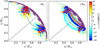Fig. 1. Slices along a constant meridian of the point-to-point 3D travel-time difference kernel for ur (left) and uθ (right). The 3D kernel for uϕ is zero along this slice. The kernel is computed with r1 and r2 separated by 42°, with mean latitude 40°. The green line is the ray path between the two points and the dashed black line shows the image plane of Fig. 2.

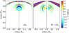Fig. 2. Slices of the point-to-point 3D travel-time difference kernel for uθ (left) and uϕ (right) along the plane indicated in Fig. 1. The 3D kernel for ur is mostly zero within this plane. The kernel is computed with r1 and r2 separated by 42°, with mean latitude 40°. The green cross indicates the intersection of the ray path and the image plane. The dashed black line shows the image plane of Fig. 1.

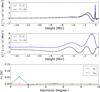Fig. 3. Top and middle panels: comparison of the kernels for $\overline{\ell }=5$ and 10 (blue and black, respectively) computed using the method here (solid lines) and the method of Gizon et al. (2017; dots). Bottom panel: travel times $\delta {\tau }_{\overline{\ell }}$ due to the radial (red) and the latitudinal (green) components of the flow for each $\overline{\ell }$ of the kernels presented here (solid line) and those of Gizon et al. (2017; dots).

2.6. Computation of kernels for meridional flow

As a first test, we compute the kernels that are required to interpret meridional flow measurements. As the flow varies slowly with latitude, we can limit the number of spherical harmonic coefficients of the kernels to $\overline{\ell }\le 10$ (see Fig. 3). As for the observations, a low-pass filter with ℓ_max = 300 is applied to the Green’s function. The method can be parallelized in $\overline{\ell }$ so we use 11 cores to compute kernels up to $\overline{\ell }=10$.

For meridional flow measurements, the separation distance between the source and the receiver is generally prescribed for different values of the mean latitude (see, e.g., Liang et al. 2017). For a given separation distance, we compute 15 kernels corresponding to 15 different latitudes. We then vary the separation distance in order to probe different depths.

Table 2 shows the computational times and memory requirements of the different steps of the algorithm. The computation of the Green’s function for a source located at the pole can be done once and for all and stored as it is necessary to do it for every kernel. Therefore, the computation is very fast (3 seconds per frequency for ℓ_max = 300) and embarrassingly parallel in frequency so it could also be recomputed every time. The computation of the frequency integrals (f^j and g^j) consists in loading the Green’s function and the weighting function W and summing over frequencies. The reading of the Green’s function files for all frequencies takes most of the time. The spatial integrals I_r, I_θ, and I_ϕ can be computed once and stored for future use. However, the computational time is small compared to the full computation of the kernel, so we decide to recompute I_j every time as the reading time can depend upon file system I/O load. The computations are parallelized in $\overline{\ell }$ and hence need 11~cores for each step since $0\le \overline{\ell }\le 10$. The computation of the kernel for u_r is faster since the computation of I_r requires the evaluation of only two Wigner-3j symbols, unlike I_θ. However, the major difference in computational time between K_r and K_θ comes from the sum in ℓ′ in Eq. (19). For K_r, the sum covers the range from $\ell -\overline{\ell }$ to $\ell +\overline{\ell }$, since I_r = 0 for other values due to the properties of the Wigner-3j. On the contrary, the sum in ℓ′ for the computation of K_θ must be computed for the full range from 0 to ℓ.

Even though the computational burden of K_θ is greater than K_r, the total burden remains significantly lower than for other methods (see Table 3). All the kernels required to perform a meridional flow inversion can be computed within 2 h with 100 cores, and the memory requirements do not exceed 1 GB. The approach mentioned in Sect. 2.3, where the full 3D kernel is computed and rotated to obtain different latitudes, would take 11 days using 1000 cores with very significant memory requirements. In the axisymmetric approach of Gizon et al. (2017) the computational time would be about 40 days on 1000 cores for all the same set of kernels.

The computational times presented here are for point-to-point measurements; however, this framework can easily be extended to geometric averaging such as arc-to-arc measurements often performed for meridional flow measurements (e.g., Liang et al. 2017). It is only necessary to replace the product of the two spherical harmonics in Eq. (19) by a sum over all the points of the arc.

2.7. Computation of kernels for supergranulation

Resolving smaller scale flows such as supergranules requires a high spatial resolution, and thus the Green’s function needs to include much higher harmonic degrees than for meridional flow Green’s function. For example, Duvall & Hanasoge (2013) considered measurements up to ℓ_max = 700, but even higher ℓ_max values may be required. Furthermore, supergranulation flows have maximum power around ℓ = 120, thus the kernels should at least be computed up to $\overline{\ell }=300$, or higher depending on the power distribution of the flow at large ℓ. The computational burden for these kernels is summarized in Table 4. The computation of the m = 0 component of the Green’s function now takes about 23 second per frequency, and the loading of the files to compute f^j around 6 min. The computation of the Wigner symbols is computationally more challenging as ℓ increases, since the number of loops scales as ${\ell }_{\max }^3$ due to loops in ℓ, ℓ′, and m. While the computation of I_r is still fast, the evaluation of I_θ now takes 270 min on 100 cores. Computing a set of 200 kernels would take 3 days with 1000 cores, which is significantly longer than for the meridional flow kernels, but still one order of magnitude faster than the approach of Gizon et al. (2017) and with a smaller memory requirement.

3. Conclusions

We presented a technique that is faster than previous approaches used to compute travel-time kernels under the assumption that the background medium is spherically symmetric. This technique does not rely on the numerical computation of kernel rotations and thus the memory requirements are small. Instead, the spatial integrals are performed analytically, which also leads to higher accuracy. For example, for meridional circulation applications, the kernels can be computed one thousand times faster than with previous methods, using a tenth of the memory requirement.

Acknowledgments

The computer infrastructure was provided by the German Data Center for SDO funded by the German Aerospace Center (DLR) and by the Ministry of Science of the State of Lower Saxony, Germany.

Appendix A

Algorithm for the integral of three associated Legendre polynomials

For the sake of completeness, we summarize the algorithm of Dong & Lemus (2002) adapted to this study. The integral of three associated Legendre polynomials,

$$J_{\ell {\ell }^{\prime }\overline{\ell }}^{m{m}^{\prime }\overline{m}}={\displaystyle {\int }_0^{\mathrm{\pi }}{P}_{\ell }^m}(\cos \theta )P_{{\ell }^{\prime }}^{m^{\prime }}(\cos \theta )P_{\overline{\ell }}^{\overline{m}}(\cos \theta )\sin \theta \mathrm{d}\theta ,$$(A.1)

can be computed analytically in terms of sums of products of Wigner-3j symbols

$$\begin{array}{ll}{J}_{\ell {\ell }^{\prime }\overline{\ell }}^{m{m}^{\prime }\overline{m}}\hfill & =\frac{{(-1)}^{\overline{m}}{(2\mathrm{\pi })}^{3/2}}{{\alpha }_{\ell }{\alpha }_{{\ell }^{\prime }}{\alpha }_{\overline{\ell }}}{\displaystyle \sum _{{\ell }_{12}=\min (|\ell -{\ell }^{\prime }|,m_{12})}^{\ell +{\ell }^{\prime }}{Q}_{12}}\hfill \\ \times \hfill & {\displaystyle \sum _{{\ell }_{123}=\min (|{\ell }_{12}-\overline{\ell }|,m_{123})}^{{\ell }_{12}+\overline{\ell }}{Q}_{123}}\sqrt{\frac{({\ell }_{123}-m_{123})!}{({\ell }_{123}+m_{123})!}}J({\ell }_{123},m_{123}),\hfill \end{array}$$(A.2)

where the indices m₁₂ = m + m′ and $m_{123}=m+m^{\prime }+\overline{m}$ represent sums over the azimuthal degrees. The quantities Q₁₂ and Q₁₂₃ must be evaluated for various values of ℓ₁₂ and ℓ₁₂₃ as defined under the sums in Eq. (A.2). They depend on the Wigner-3j symbols:

$$\begin{array}{lll}{Q}_{12}\hfill & =\hfill & (2{\ell }_{12}+1)\left(\begin{array}{ccc}\ell & {\ell }^{\prime }& {\ell }_{12}\\ 0& 0& 0\end{array}\right)\left(\begin{array}{ccc}\ell & {\ell }^{\prime }& {\ell }_{12}\\ m& m^{\prime }& -m_{12}\end{array}\right),\hfill \\ Q_{123}\hfill & =\hfill & (2{\ell }_{123}+1)\left(\begin{array}{ccc}{\ell }_{12}& \overline{\ell }& {\ell }_{123}\\ 0& 0& 0\end{array}\right)\left(\begin{array}{ccc}{\ell }_{12}& \overline{\ell }& {\ell }_{123}\\ m_{12}& \overline{m}& -m_{123}\end{array}\right).\hfill \end{array}$$

The value of Q₁₂ (resp. Q₁₂₃) is non-zero only if ℓ₁₂ + ℓ + ℓ′ (resp. ${\ell }_{12}+\overline{\ell }+{\ell }_{123}$) is even. The last term J(ℓ₁₂₃, m₁₂₃) is the integral

$$J({\ell }_{123},m_{123})={\displaystyle {\int }_{-1}^1{P}_{{\ell }_{123}}^{m_{123}}(x)\mathrm{d}x,}$$(A.3)

which can be evaluated analytically. In this paper, we only need this value for m₁₂₃ = ± 1. As this integral is zero for odd values of ℓ₁₂₃, due to the parity of the associated Legendre polynomials, we set ℓ₁₂₃ = 2p + 1. Then, for a given m₁₂₃, the value of J(ℓ₁₂₃, m₁₂₃) can be evaluated recursively using

$$J(2n+1,1) =\frac{(2n+1)(2n-1)}{4n(n+1)}J(2n-1,1)$$(A.4)

and

$$\mathrm{\hspace{0.17em}}J(2n+1,-1) =\frac{{(2n-1)}^2}{4{(n+1)}^2}J(2n-1,-1),$$(A.5)

where n = 1, 2, ... p, together with the initial conditions

$$J(1,1)=-\frac{\mathrm{\pi }}{2}\mathrm{\hspace{0.17em}}\mathrm{ and }\mathrm{\hspace{0.17em}}J(1,-1)=\frac{\mathrm{\pi }}{4}.$$(A.6)

References

All Tables

All Figures

	Fig. 1. Slices along a constant meridian of the point-to-point 3D travel-time difference kernel for ur (left) and uθ (right). The 3D kernel for uϕ is zero along this slice. The kernel is computed with r1 and r2 separated by 42°, with mean latitude 40°. The green line is the ray path between the two points and the dashed black line shows the image plane of Fig. 2.
In the text

Fig. 2. Slices of the point-to-point 3D travel-time difference kernel for uθ (left) and uϕ (right) along the plane indicated in Fig. 1. The 3D kernel for ur is mostly zero within this plane. The kernel is computed with r1 and r2 separated by 42°, with mean latitude 40°. The green cross indicates the intersection of the ray path and the image plane. The dashed black line shows the image plane of Fig. 1.

In the text

Fig. 3. Top and middle panels: comparison of the kernels for $\overline{\ell }=5$ and 10 (blue and black, respectively) computed using the method here (solid lines) and the method of Gizon et al. (2017; dots). Bottom panel: travel times $\delta {\tau }_{\overline{\ell }}$ due to the radial (red) and the latitudinal (green) components of the flow for each $\overline{\ell }$ of the kernels presented here (solid line) and those of Gizon et al. (2017; dots).

In the text

References

- Birch, A. C., & Kosovichev, A. G. 2000, Sol. Phys., 192, 193 [NASA ADS] [CrossRef] [Google Scholar]
- Birch, A. C., Kosovichev, A. G., & Duvall,Jr., T. L., 2004, ApJ, 608, 580 [NASA ADS] [CrossRef] [Google Scholar]
- Böning, V. G., Roth, M., Zima, W., Birch, A. C., & Gizon, L. 2016, ApJ, 824, 14 [Google Scholar]
- Burston, R., Gizon, L., & Birch, A. C., 2015, Space Sci. Rev., 196, 201 [Google Scholar]
- Chabassier, J., & Duruflé, M. 2016, High Order Finite Element Method for Solving Convected Helmholtz Equation in Radial and Axisymmetric Domains. Application to Helioseismology, INRIA, Research Report RR- 8893 [Google Scholar]
- Christensen-Dalsgaard, J., Dappen, W., Ajukov, S. V., et al. 1996, Science, 272, 1286 [CrossRef] [Google Scholar]
- DLMF. 2017, NIST Digital Library of Mathematical Functions, http://dlmf.nist.gov/, Release 1.0.16 of 2017-09-18, eds. f. W. J. Olver, A. B. Olde Daalhuis, D. W. Lozier, et al. [Google Scholar]
- Dong, S.-h., & Lemus, R. 2002, Appl. Math. Lett., 15, 541 [CrossRef] [Google Scholar]
- Duvall, T., Jeffferies, S., Harvey, J., & Pomerantz, M. 1993, Nature, 362, 430 [NASA ADS] [CrossRef] [Google Scholar]
- Duvall, T. L., & Hanasoge, S. M. 2013, Sol. Phys., 287, 71 [NASA ADS] [CrossRef] [Google Scholar]
- Edmonds, A. R. 1960, Angular Momentum in Quantum Mechanics (Princeton University Press) [Google Scholar]
- Fournier, D., Leguèbe, M., Hanson, C. S., et al. 2017, A&A, 608, A109 [CrossRef] [EDP Sciences] [Google Scholar]
- Gizon, L., & Birch, A. 2002, ApJ, 571, 966 [NASA ADS] [CrossRef] [Google Scholar]
- Gizon, L., Barucq, H., Duruflé, M., et al. 2017, A&A, 600, A35 [NASA ADS] [CrossRef] [EDP Sciences] [Google Scholar]
- Kosovichev, A. G. 1996, ApJ, 461, L55 [NASA ADS] [CrossRef] [Google Scholar]
- Kosovichev, A. G., Duvall,Jr., T. L.,, & Scherrer, P. H. 2000, Sol. Phys., 192, 159 [NASA ADS] [CrossRef] [Google Scholar]
- Liang, Z.-C., Birch, A. C., Duvall,Jr., T. L., Gizon, L., & Schou, J. 2017, A&A, 601, A46 [NASA ADS] [CrossRef] [EDP Sciences] [Google Scholar]
- Mandal, K., Bhattacharya, J., Halder, S., & Hanasoge, S. M. 2017, ApJ, 842, 89 [NASA ADS] [CrossRef] [Google Scholar]
- Nagashima, K., Fournier, D., Birch, A. C., & Gizon, L. 2017, A&A, 599, A111 [NASA ADS] [CrossRef] [EDP Sciences] [Google Scholar]
- Rajaguru, S., & Antia, H. 2015, ApJ, 813, 114 [NASA ADS] [CrossRef] [Google Scholar]
All Tables
Computational time of the different steps to obtain 15 flow kernels (15 latitudes) for a given separation distance with and ℓmax = 300 using 11 cores.
Comparison of the computational time and memory requirements to evaluate 225 kernels for the meridional flow.
Computational time of the different steps to obtain 15 flow kernels for a given separation distance with and using 100 cores.