| Issue |
A&A
Volume 616, August 2018
|
|
|---|---|---|
| Article Number | A157 | |
| Number of page(s) | 10 | |
| Section | Extragalactic astronomy | |
| DOI | https://doi.org/10.1051/0004-6361/201833114 | |
| Published online | 07 September 2018 | |
Probing star formation and ISM properties using galaxy disk inclination
II. Testing typical FUV attenuation corrections out to z ~ 0.7⋆
1
Max-Planck-Institut für Astronomie, Königstuhl 17, 69117 Heidelberg, Germany
e-mail This email address is being protected from spambots. You need JavaScript enabled to view it.
2
Research School of Astronomy and Astrophysics, Australian National University, Canberra ACT 2611, Australia
3
Astronomy Centre, Department of Physics and Astronomy, University of Sussex, Brighton BN1 9QH, UK
4
INAF-Osservatorio Astronomico di Bologna, via Gobetti 93/3, 40129 Bologna, Italy
5
Argelander-Institut für Astronomie, Auf dem Hügel 71, 53121 Bonn, Germany
Received:
27
March
2018
Accepted:
11
May
2018
Abstract
We evaluate dust-corrected far-ultraviolet (FUV) star formation rates (SFRs) for samples of star-forming galaxies at z ~ 0 and z ~ 0.7 and find significant differences between values obtained through corrections based on UV colour, from a hybrid mid-infrared (MIR) plus FUV relation, and from a radiative transfer based attenuation correction method. The performances of the attenuation correction methods are assessed by their ability to remove the dependency of the corrected SFR on inclination, as well as returning, on average, the expected population mean SFR. We find that combining MIR (rest-frame ~ 13 μm) and FUV luminosities gives the most inclination-independent SFRs and reduces the intrinsic SFR scatter of the methods we tested. However, applying the radiative transfer based method also gives corrections to the FUV SFR that are inclination independent and in agreement with the expected SFRs at both z ~ 0 and z ~ 0.7. SFR corrections based on the UV-slope perform worse than the other two methods we tested. For our local sample, the UV-slope method works on average, but does not remove inclination biases. At z ~ 0.7, we find that the UV-slope correction we used locally flattens the inclination dependence compared to the raw FUV measurements, but was not sufficient to correct for the large attenuation observed at z ~ 0.7.
Key words: galaxies: star formation / ultraviolet: galaxies / galaxies: evolution / galaxies: ISM
Tables of the computed SFRs are only available at the CDS via anonymous ftp to cdsarc.u-strasbg.fr (130.79.128.5) or via http://cdsarc.u-strasbg.fr/viz-bin/qcat?J/A+A/616/A157
Fellow of the International Max Planck Research School for Astronomy and Cosmic Physics at the University of Heidelberg (IMPRS-HD).
© ESO 2018
1. Introduction
Robust measurements of star formation rates (SFR) are a key ingredient in the context of galaxy evolution studies. The farultraviolet (FUV; ~ 1550 Å) is dominated by radiation from O and B stars and thus traces recent star formation, provided the timescale for significant fluctuations is longer than a few 107 years (Madau & Dickinson 2014). Extragalactic UV SFR calibrations have been revolutionised by the launch of the Galaxy Evolution Explorer mission (GALEX; Martin et al. 2005), which imaged approximately two-thirds of the sky at FUV and near-UV (NUV) wavelengths. Murphy et al. (2011) and Hao et al. (2011) used the Starburst99 stellar population synthesis code (Leitherer et al. 1999) to derive conversions between GALEX FUV luminosity and SFR at an age of 100 Myr, assuming a constant SFR and solar metallicity: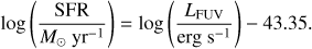 (1)
(1)
The great disadvantage for UV-based SFR measurements is that the light is heavily attenuated by dust. When stars are not individually resolved, the effective reddening of the emerging radiation is influenced by the dust–stars–gas geometry of the observed region (Natta & Panagia 1984; Calzetti 1997). Furthermore, the reddening laws are not the same for all galaxies, nor for regions within galaxies, due to a combination of different dust grain size distributions and compositions, and differing geometries. The amount of unattenuated starlight is negligible in dusty starbursts, but is almost 100% in dust-poor dwarf galaxies.
Dust is present in stellar birth clouds and in the diffuse interstellar medium, and both components absorb starlight and re-emit it in the infrared (IR). However, the dust–star geometry appears to evolve with redshift, with results from paper I in this series (Leslie et al. 2018, L18) indicating that the fraction of dust in stellar birth clouds was higher at earlier times (z ~ 0.7).
To infer dust-unbiased, total SFRs, corrections accounting for UV attenuation are necessary. A promising way to obtain the total SFR of a galaxy is to combine the UV emission with infrared emission, thereby capturing both the attenuated and unattenuated emission. Combined UV+IR SFRs have been used with success out to at least z < 3 (Wuyts et al. 2011; Santini et al. 2014; Magnelli et al. 2014). However, older stellar populations can contribute to dust heating and infrared emission (Bendo et al. 2010; Groves et al. 2012). Therefore, the exact relation between infrared emission and recent SFR will depend on the relative contribution of the young and old stellar populations to the general stellar radiation field, which varies from galaxy to galaxy, see for example Boquien et al. (2016).
Corrections at high redshift (z > 2) often rely on empirical calibrations based on the UV spectral slope or UV colours. However, these calibrations are uncertain due to potential intrinsic variations in the UV slope and dust attenuation (Battisti et al. 2016; Salmon et al. 2016) Further testing of the UV slope and hybrid UV + IR attenuation correction methods are still required, particularly to ascertain that they are applicable at z > 0.
We can evaluate UV-attenuation corrections by testing whether the corrected SFR is independent of galaxy inclination. Inclined galaxies suffer from more line-of-sight attenuation than face-on galaxies because light has a larger column to pass through before escaping the galaxy. An ideal correction would account for this extra attenuation and result in a total SFR that is independent of viewing angle. In L18, we used the inclination–SFR (uncorrected for attenuation) relation of star-forming galaxies at different wavelengths (UV, mid-IR, far-IR, and radio) to probe the disc opacity of two matching samples of massive (M⋆ > 1.6 × 10¹⁰ M⊙), large (r1/2 > 4 kpc), disc-dominated (n < 1.2) galaxies: a local Sloan Digital Sky Survey (SDSS) sample at z ~ 0.07 and a sample of discs at z ~ 0.7 drawn from the Cosmic Evolution Survey (COSMOS). We found that correcting the FUV flux for dust attenuation is critical even for face-on galaxies because the observed UV fluxes can underestimate the true SFR by a factor of ~ 1.6 for face-on massive star-forming galaxies at z ~ 0 and ~ 5.5 at z ~ 0.7.
In this paper we test the inclination dependence of UV-derived SFRs that have been corrected for attenuation using common empirical approaches: UV-slope corrections (Sect. 3.1), hybrid UV+MIR SFRs (Sect. 3.2), and SFRs corrected for the attenuation expected from the radiative transfer model of Tuffs et al. (2004) and Popescu et al. (2011) (Sect. 3.3). We apply these attenuation corrections to two samples of massive starforming galaxies, ~ 3500 galaxies at z ~ 0 and ~ 1000 galaxies at ~ 0.7, and test for inclination dependence following the methodology of L18.
Throughout this work, we use the Kroupa (2001) initial mass function (IMF) and assume a flat Λ cold dark matter (CDM) cosmology with (H0, ΩM, ΩΛ ) = (70 km s−1 Mpc−1, 0.3, 0.7).
2. Data and sample selection
L18 described the data and sample selection, which we only briefly review here. We selected a local sample (0.04 < z < 0.1) from the spectroscopic SDSS matched with the GALEX Medium Imaging Survey (MIS) by Bianchi et al. (2011). Our intermediate-redshift sample (0.6 < z < 0.8) from the COSMOS field is centred at z ~ 0.7, where we have high-resolution restframe morphological measurements in the I band (Sargent et al. 2007) that match our SDSS g-band morphological measurements (Simard et al. 2011) in terms of rest-frame wavelength. Additionally, the GALEX NUV filter at z ~ 0.7 matches the FUV filter at z ~ 0.1, ensuring that our FUV fluxes obtained from the GALEX Deep Imaging Survey (DIS) do not require k corrections.
L18 found that inclination affects the derived galaxy properties that are used for sample selection. After fitting and subtracting a power law from the relations of inclination versus galaxy property for M⋆, g-band half-light radius r1/2, and Sérsic index n, we obtained “face-on” equivalent values for each galaxy. The inclination-corrected parameters, denoted with the subscript “corr”, were only used for sample selection. Our selections from L18 are as follows and are referred to as the “restricted” sample:
-
log(M⋆,corr/M⊙) > 10.2,
-
ncorr < 1.2,
-
r1/2,corr > 4 kpc
-
LFUV/σLFUV > 3.
Star-forming galaxies were selected using their emission line ratios or colours for the local and COSMOS samples, respectively. The restricted sample contains 1021galaxies in the local sample and 295 galaxies in the z ~ 0.7 sample. The size cut ensures completeness in surface brightness, and the Sérsic index cut reduces contamination by bulge-dominated galaxies. However, to make our results applicable to a wider population of galaxies, we also present results for a sample that is not subject to size restrictions and has a less restrictive constraint on the Sérsic index:
-
log(M⋆,corr/M⊙) > 10.2,
-
ncorr < 2
-
LFUV/σLFUV > 3.
We refer to this sample as the “full” sample, and it contains 3489 galaxies at z ~ 0 and 575 galaxies at z ~ 0.7. Before requiring an FUV detection at a signal-to-noise ratio >3, the full local sample contains 8576 galaxies and the full COSMOS sample contains 1135 galaxies. Although the signal-to-noise ratio cut biases the sample towards galaxies with higher SFRs, it is necessary for reliable results. In our COSMOS sample we are likely missing the most highly inclined (1 − cos(i) > 0.75; i = 75.5°) galaxies with lower SFRFUV because of the sensitivity limit of GALEX DIS data.
In addition to the previous UV and MIR samples of L18, we also include here a UV-slope-corrected sample (Sect. 3.1), which requires the addition of rest-frame NUV data. This results in a smaller subsample, especially at z ~ 0.7 (Table 1).
Best-fit parameters of the relation log SFRFUV,corr/SFRMS(M⋆, z)) = k1(1 − cos(i)) + k2, where SFRFUV,corr is measured using three different methods.
3. Corrected FUV star formation rates, SFRFUV,corr
In this section, we apply three common SFRFUV attenuation corrections to test whether any residual trends of SFR with inclination persist.
We chose to normalize the SFRUV,corr by the SFR expected for a galaxy lying exactly on the galaxy SFR–stellar mass relation (galaxy main-sequence, MS). As in L18, we adopted the best-fit MS relation for an updated version of the z ≲ 1 data compiled in Sargent et al. (2014, and priv. comm.),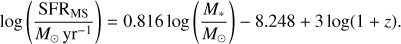 (2)
(2)
We took into account the different IMF (Chabrier 2003) and cosmology (WMAP-7; Larson et al. 2011) assumed by (Sargent et al. 2014; see L18 for more details). Figure 1 shows the relation between log(SFRFUV,corr/SFRMS) and galaxy inclination (1 − cos(i)), where SFRMS is the main-sequence SFR expected given the mass and redshift of each galaxy.
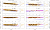 |
Fig. 1. Evaluating the inclination dependence of dust-corrected SFRFUV values. From top to bottom, the panels show the observed UV SFR, the SFR corrected based on the UV-slope, the hybrid MIR+UV determined SFR, and the SFR corrected based on the Tuffs et al. (2004) radiative transfer models as a function of inclination angle. Face-on galaxies are lie to the left, 1 − cos(i) ~ 0, and edge-on galaxies lie to the right, 1 − cos(i) ~ 1. The blue lines show the inclination relation for SFRFUV as observed with no dust corrections (top panel). The dust correction factors work to increase the SFRFUV and lessen the inclination dependence of the SFR. Fitted parameters are given in Table 1. Orange data points show the “restricted sample”, and the full sample is shown as a 2D density histogram. Magenta lines show 150 random realisations of linear parameters from our MCMC chain. Distributions of the y-axes, log(SFRFUV/SFRMS) are also displayed as histograms. The dotted line shows where the SFRFUV = SFRMS. |
The fits shown in Fig. 1 are of the form (3)
(3)
Best fits were obtained using the Monte Carlo Markov chain implementation emcee (a PYTHON package) (Foreman-Mackey et al. 2013), incorporating errors on the SFRs and inclination and fitting for an intrinsic variance term, σ2, following Foreman-Mackey (2017). For simplicity, the intrinsic scatter was assumed to be in the y-direction only (SFR). We used 64 walkers that created a chain of 6000 samples each for a total of 340 000 samples. The first 150 samples were discarded as an initialisation period (burn-in). The fitted parameters for the original uncorrected and corrected SFR relations are shown in Table 1, where we give the median, and the 5th and 95th percentile of the MCMC distribution.
The top panels of Fig. 1 show the observed SFRFUV. The restricted samples span the same range of inclinations as the larger full samples. However, the restricted samples tend to be skewed towards higher SFRFUV values, showing a lack of SFRFUV,obs at all inclinations. The restricted samples’ galaxies are larger and more disc dominated than the full samples. These values indicate a mean attenuation factor of A FUV ~ 1.9 mag (~1.5 mag) at z ~ 0 and A FUV ~ 2.9 mag (~2.4 mag) at z ~ 0.7 for the full (restricted) samples.
The fitted slope of the SFRFUV-inclination for the COSMOS (−0.44 ± 0.15) and local (−0.9 ± 0.06) restricted samples differ from the slopes found in L18 (−0.54 ± 0.09 and −0.79 ± 0.04 for the COSMOS and SDSS samples, respectively) because different fitting methods were adopted. The fitting algorithm in this work is more lenient towards outliers, but was selected in order to evaluate the scatter of our SFR values before and after corrections. We chose to test the correction methods described below, which are representative of those commonly applied in the literature.
3.1. UV slope correction
The observed relationship between the rest-frame UV continuum slope β, where Fλ ∝ λβ, and the ratio of UV to IR light of a galaxy (IRX, log(LIR/LUV)) has been used to calibrate β as an attenuation correction tool since the correlation was first observed for starburst galaxies by Meurer et al. (1999) and Calzetti (1997). Longer-lived (~200 Myr), lower-mass stars contribute substantially to the NUV emission at later times. For a constant SFR, the UV spectral slope therefore reddens moderately with time, complicating the conversion from luminosity into SFR. For this analysis we estimated β by fitting log(Fλ) = βlog(λ(1+z))+c using the PYTHON package POLYFIT, with data weighted by their flux errors. For our SFRFUV,corr error values, we used and propagated the errors on the fitted slope given by POLYFIT. When only two data points were available, we calculated the gradient and the corresponding error. We then used the Boquien et al. (2012) relation (see their Sect. 4.2), (4)
(4)
to determine the amount of attenuation and correct SFRFUV. We were unable to avoid photometric bands with emission or absorption lines, as suggested for example by Calzetti et al. (1994), which increases the uncertainty β. However, Leitherer et al. (2011) found a good agreement between UV spectral slopes determined from International Ultraviolet Explorer spectra and from the GALEX FUV and NUV magnitudes of nearby galaxies. The A FUV–β relation in Eq. (4) was derived for normal face-on star-forming spiral galaxies. This relation varies from that of starburst galaxies (e.g. Overzier et al. 2011; Meurer et al. 1999), largely due to intrinsic UV colour differences between galaxies and yields systematically lower attenuation for a given β. Observations of a wide range of galaxies have shown a large scatter in the UV colour-extinction relation (Boquien et al. 2012) and about two orders of magnitudes of scatter in actual FUV attenuations for a fixed FUV–NUV colour. Studies such as Catalán-Torrecilla et al. (2015) have shown that even with a UV colour correction, the FUV alone is not a reliable tracer of SFR in individual galaxies. This is because of the large extinction correction needed at FUV wavelengths, and the variation of different attenuation laws in the UV.
Local sample: For our SDSS sample, we have access to photometry from only two UV bands: GALEX NUV (λeff = 2274 Å) and FUV (λeff = 1542 Å). Using AFUV, we corrected the observed LFUV used to calculate SFR in Eq. (1) and show the trend of SFRFUV,corr with the inclination in Fig. 1. Figure 2 shows the distribution of β, peaking close to β ~ −1 for both the full and restricted samples.
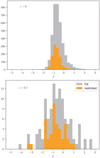 |
Fig. 2. UV-slope, β, distribution for restricted (orange) and full samples (grey) in our local sample (top panels) and z ~ 0.7 sample (bottom panels). |
The colour-corrected SFRFUV show a slightly shallower inclination dependency (slope of −0.8 ± 0.02 instead of −1.0 ± 0.03 for the full sample, and −0.79 ± 0.03 instead of −0.9 ± 0.04 for the restricted sample) and overall SFRs that are closer to the MS, but further improvements are required because the slopes are significantly different from zero and one will tend to over-estimate the SFR for face-on galaxies and under-estimate the SFR for edge-on galaxies.
COSMOS sample: For the COSMOS sample, we fit the UV spectral slope β using flux densities observed between rest-frame 1250–2500 Å. For our redshift range, this corresponds to the COSMOS2015 B, IB427, u, or GALEX NUV bands. To fit the spectral slope, we did not use flux values with a flag >0 (Laigle et al. 2016). Our data show β values ranging between 2 and −3, with most galaxies having β ~ −0.8 for both the full and restricted samples.
The limiting factor is the small number of photometric data points in the rest-frame wavelength range 1250–2500 Å over our redshift range. For z < 0.705, only the NUV and u band lie in the rest-frame 1250–2500 Å range. Between 0.70 < z < 0.78, the IB427 band can also be used to constrain β, and for 0.78 < z < 0.8, we can use the u, IB247, and the B band along with GALEX NUV to constrain β. No redshift dependency on our fitted β slopes arises because different bands were used for the full and restricted samples.
The SFRFUV corrected for attenuation using the spectral slope appears to remove most of the inclination dependence at z ~ 0.7. The slopes are 0.05 ± 0.45 for the full sample and −0.05 ± 0.51 for the restricted sample; however, these slopes are poorly constrained because of the small number of galaxies (56 in the full and 28 in the restricted samples, respectively) with robust β measurements at z ~ 0.7. The average SFR has also increased, but the corrected values are still below the MS by −0.46 ± 0.20 dex for the full sample and −0.12 ± 0.25 dex for the restricted sample for face-on galaxies. Figure 2 shows the distribution of β is very similar for the z ~ 0.7 and z ~ 0 samples, peaking around β ~ −1.
In Appendix A we explore the effects of assuming a constant attenuation factor of AV = 1 for all galaxies in the COSMOS sample. Assuming a constant factor is, in some cases, the only way to build a statistically significant sample of galaxies with SFR measurements. While this assumption ignores any inclination effects, it can correct the systematic offset observed in the top right panel of Fig. 1. We also show the results for an alternative AFUV–β relation from Wang et al. (2016) in Appendix A.
3.2. MIR hybrid correction
The most widely used composite tracers combine the UV observations with IR measurements using an energy-balancing approach that in the simple case assumes that the IR and UV light comes from a similar optical depth. This is generally a valid assumption and means that a linear combination of observed LFUV and LIR luminosity can correct the UV fluxes for dust attenuation (Kennicutt et al. 2009; Hao et al. 2011; Catalán-Torrecilla et al. 2015), (5)
(5)
The coefficient η can be calibrated theoretically with evolutionary synthesis models or empirically using independent measurements of dust-corrected SFRs (Treyer et al. 2010; Hao et al. 2011). In most cases, η < 1 because dust is significantly heated by old stars and by emission arising from the IR cirrus. Different sample selections result in different determinations of η because of different contributions of the old and young stellar populations in the dust-heating, inter-stellar radiation field. For example, early studies were restricted to luminous starburst galaxies and star-forming regions (e.g. Buat et al. 1999; Meurer et al. 1999), and yielded values of ~ 0.6 (Kennicutt & Evans 2012). With the advent of GALEX, Spitzer, and Herschel, subsequent analyses of normal star-forming galaxies typically find lower η values, for instance Hao et al. (2011), and Wang et al. (2016; although see Boquien et al. 2016). In this analysis, we have access to MIR fluxes through WISE (local sample) and Spitzer-MIPS (COSMOS sample). The MIPS 24 μm data samples rest-frame 14 μm fluxes at z ~ 0.7. The short-wavelength MIR range (~3–20 μm) dust emission arises from strong polycyclic aromatic hydrocarbon (PAH) emission features and continuum (Leger & Puget 1984; Allamandola et al. 1985; Dopita et al. 2003; Smith et al. 2007). The continuum emission comes from both single-photon, stochastically heated small dust grains (typically <0.01 μm) and from thermally emitting hot (T > 150 K) dust (Calzetti 2013).
We correct the UV luminosity following Hao et al. (2011)
 (6)
(6)
For our analysis we adopted SFRFUV,corr errors given by the uncertainties on the UV and MIR fluxes alone. However, we note that η has been found to vary with stellar mass and morphological type by up to factors of 4 for local late-type galaxies (Boquien et al. 2016; Catalán-Torrecilla et al. 2015).
Local sample. The WISE W3 band is broad, covering 7.5–16.5 μm at half-power (Jarrett et al. 2011). This wavelength range encompasses multiple PAH features as well as H2 and forbidden neon emission lines. PAH fractions tend to be high in regions of active star formation, and the WISE 12 μm emission has been shown to correlate well with SFR (Cluver et al. 2014, 2017). We followed the method in L18 to convert the W3 flux into total infrared luminosity using the spectral energy distribution (SED) template of Wuyts et al. (2008). Additionally, we discuss the use of other monochromatic-to-total infrared (TIR) calibrations making use of WISE 12 μm and 22 μm data in Appendix B.
We then corrected our LFUV according to Eq. (6) and calculated SFRFUV,corr. The resulting SFRFUV,corr values show very little inclination dependence on slopes k 1 = − 0.15 ± 0.03 and −0.21 ± 0.05 for the full and restricted samples, respectively. The fitted intrinsic scatter of the hybrid SFR-inclination relation is smaller than the other local SFR-inclination relations. The corrected SFRs of face-on galaxies lie above the expected SFRMS by 0.15 ± 0.02 and 0.14 ± 0.02 dex for the edge-on and face-on samples, while the corrected SFRs of edge-on galaxies are entirely consistent with the MS.
COSMOS sample. For the COSMOS sample, we have 24 μm flux measurements, or rest-frame ~ 14 μm. We followed the method in L18 to convert this flux into total infrared luminosity (using the SED template of Wuyts et al. 2008). The resulting hybrid SFRFUV,corr – inclination relation has a slope consistent with zero for both the full and restricted subsamples. The y-intercept values are also low: −0.16 ± 0.09 and −0.03 ± 0.06 for the full and restricted samples, respectively. For the COSMOS hybrid corrections, the restricted sample has, on average, slightly higher SFRFUV,corr than the full sample. The scatter is not reduced as significantly as it was in the local sample for the hybrid SFRs, but is still the smallest out of the four SFRFUV – inclination relations shown. Other authors such as Izotova & Izotov (2018) also found a smaller scatter in the MIR+UV hybrid SFRs than for SFRs derived from either of the original UV or MIR bands.
3.3. Radiative transfer correction
Integrated SED models fitted to observations can constrain physical properties of a galaxy, including the SFR. The radiative transfer (RT) method self-consistently calculates the dust emission SED based on the radiation field of the attenuated stellar population. When creating model SEDs using the RT method, the geometry and distribution of the stars, dust, and gas in the galaxy can be determined either from a hydrodynamical model or a toy model of the galaxy. In L18, SFRFUV,obs-inclination relations were fit with the model predictions of the Tuffs et al. (2004) RT calculations based on a simple geometric model for a spiral galaxy. For the UV attenuation calculations, it was assumed that UV emission comes only from the thin disc of a galaxy, simplifying the calculation by removing the bulge or thick-disc stellar model components. Under this assumption, the parameters required for the model are inclination angle, B-band opacity through the centre of the galaxy as seen face-on ( ), and the fraction of stellar light locally absorbed in star-forming clouds (as opposed to being absorbed by the diffuse dust component), F.
The model of Tuffs et al. (2004) derives the attenuated stellar population, and the resulting dust emission expected was calculated in Popescu et al. (2011). Recently, Grootes et al. (2013, 2017), and Davies et al. (2016), have used RT dust corrections based on the Tuffs et al. (2004) and Popescu et al. (2011) models to correct NUV luminosities for dust attenuation.
Tuffs et al. (2004) fit the attenuation curves (the change of magnitude Δm due to dust attenuation; Δm vs 1 − cos(i)) of the thin-disc component with a fifth-order polynomial at various  values and wavelengths. We interpolated the Tuffs et al. (2004) models to derive the Δm at 1542 Å, which is the effective wavelength of the GALEX FUV filter. Then L
FUV was corrected with Δm to give SFRFUV,corr.
values and wavelengths. We interpolated the Tuffs et al. (2004) models to derive the Δm at 1542 Å, which is the effective wavelength of the GALEX FUV filter. Then L
FUV was corrected with Δm to give SFRFUV,corr.
For the errors on the SFRs corrected by this method, we adopted a constant σ = 0.09 dex as suggested by Davies et al. (2016) in their Appendix A. Davies et al. (2016) found that the RT method produces the most consistent slopes and normalisations of the SFR-M ⋆ relation out of the 12 different SFR metrics compared for local spiral galaxies1.
Local sample. We repeated our analysis of L18, Sect. 3.3, and fit the Tuffs et al. (2004) models to our full sample. We find best-fitting parameters of  . We then used these fixed parameters to correct the SFR for each galaxy, given its inclination angle. Our best-fit slope values become significantly flatter than for the uncorrected sample, being −0.01 ± 0.02 and −0.06 ± 0.06 for the full and restricted samples, respectively. However, this correction does not reduce the observed dispersion σ
2 for the full sample. By using the bestfitting parameters for the full galaxy sample to correct SFRFUV, we would expect the normalisation and intercept to be close to zero for the full sample.
. We then used these fixed parameters to correct the SFR for each galaxy, given its inclination angle. Our best-fit slope values become significantly flatter than for the uncorrected sample, being −0.01 ± 0.02 and −0.06 ± 0.06 for the full and restricted samples, respectively. However, this correction does not reduce the observed dispersion σ
2 for the full sample. By using the bestfitting parameters for the full galaxy sample to correct SFRFUV, we would expect the normalisation and intercept to be close to zero for the full sample.
Grootes et al. (2017) used an empirical relation between stellar mass surface density and B-band optical depth (Grootes et al. 2013) to set  , fixing F = 0.41 (Popescu et al. 2011). Adopting this method gives (k1k2, σ2) = (0.14 ± 0.03, 0.18 ± 0.02, 0.25 ± 0.01) for the full and (0.20 ± 0.05, 0.22 ± 0.02, 0.16 ± 0.01) for the restricted samples, respectively. This correction overestimates the FUV SFRs on average, and leaves a positive residual inclination dependency. On the other hand, adopting the Grootes et al. (2013)
 , and keeping our fitted value of F = 0.209, we find (k1, k2, σ2) = (0.14 ± 0.03, −0.03 ± 0.02, 0.26 ± 0.01) for the full sample and (0.19 ± 0.05, 0.22 ± 0.02, 0.16 ± 0.01) for the restricted sample. Naturally, using different τ values for each galaxy reduces the scatter in the SFRFUV,corr values. However, the parameters of
  and F are derived jointly in the best fit, and therefore must be set consistently with each other, as done for our adopted method in Table 1 (
 , F = 0.209 for all galaxies).
COSMOS sample. We find best-fitting parameters for the full z ~ 0.7 sample to be  and
and  . Using these values to determine the required UV attenuation correction, we obtain best-fit values that show a positive slope of 0.16 ± 0.13 and 0.16 ± 0.16 for the full and restricted samples, respectively. These slopes are different from zero at the 2 and 1.6 σ levels for the full and restricted samples, respectively; moreover, it appears that they are driven by galaxies with the highest inclination angles, where the correction is most uncertain. The intrinsic scatter has increased from the scatter of the uncorrected SFRs by this correction.
4. Discussion and conclusion
We have tested a number of global galaxy FUV attenuation correction methods for samples of massive (M ⋆ > 1.6 × 10¹⁰) galaxies at z ~ 0 and z ~ 0.7 selected to be representative of corrections applied in the literature. FUV SFRs are very difficult to properly correct for dust attenuation. Conversely, SFR calibrations at different wavelengths are sensitive to stellar populations over different timescales. SFR estimators at longer wavelengths are not able to capture variations on short timescales, leading to important discrepancies on the estimates of the instantaneous SFR. Despite these many uncertainties, we find that hybrid MIR and RT attenuation correction methods can remove the overall offset from the MS and decrease the inclination dependency of UV SFRs.
Hybrid MIR + UV SFR calibrations remove a significant fraction of the inclination dependency displayed by uncorrected SFRFUV at z ~ 0.7 and at z ~ 0. However, there is some remaining uncertainty regarding the normalisation of the calibration due to differences in IR templates and intrinsic SFRs. The scatter of SFR from galaxy to galaxy is decreased when this technique is used. We also found that the RT method of Tuffs et al. (2004) works reasonably well for correcting the normalisation and inclination dependency of SFRFUV at both z ~ 0 and z ~ 0.7 and is not highly dependent on the choice of input parameters  and F.
We find that the SFR correction methods tested give similar results, in that they perform similarly well, for both the full sample of star-forming galaxies and our restricted samples (with a cut for larger sizes and lower Sérsic indexes) of large discdominated galaxies. One difference between the samples is that the dispersion is smaller for the restricted sample at z ~ 0. This might be because the restricted sample spans a smaller range of galaxy morphologies, only including large exponential discs.
Despite the small number of galaxies detected in COSMOS at multiple UV wavelengths, we are able to learn something from the UV slope measurements at z ~ 0.7. The attenuation at higher redshift is so substantial that inclination dependency is probably not the dominant concern for the SFRFUV measurements because accurately correcting the average attenuation of the population gives the most improvement in terms of SFRs. At both z ~ 0 and z ~ 0.7, applying an attenuation correction based on the UV slope is better than no correction, but at z ~ 0.7, the SFRs on average still lie below the MS by ~ 0.44 dex and ~ 0.15 dex for the full and restricted samples, respectively (for a galaxy at 1 − cos(i) = 0.5).
L18 found that dust at z ~ 0.7 is most closely associated with star-forming clumps rather than the disc. Therefore, we expect the UV attenuation curve to be relatively constant with disc inclination angle. In the local sample, we found that adopting a single UV-slope attenuation relation was unable to remove the inclination bias. The attenuation for face-on galaxies is dominated by the clumpy dust component, whereas the attenuation for edge-on galaxies is more affected by the diffuse dust disc, and these two components have different UV-attenuation laws (e.g. Wild et al. 2011; da Cunha et al. 2008; Charlot & Fall 2000). Therefore, a different A FUV–β relation would be required at different galaxy inclinations. Perhaps at the highest inclination angles, where birth-clouds might overlap along the line of sight and photons would have to escape through more optically thick material, we might see a drop-off in FUV light. A cross-over of star-forming clouds would depend on the cloud number density. Galaxies around cosmic noon (z ~ 2) were forming stars at a faster rate, having more birth clouds. On one hand, the higher SFR would increase the probability that the birth clouds overlap along the line of sight for inclined galaxies. On the other hand, the scale-height of the gas disc is also expected to be larger at this redshift (Förster Schreiber et al. 2009; Kassin et al. 2012; Stott et al. 2016; Turner et al. 2017). A larger scale-height would dampen any expected inclination dependency. Therefore it would be interesting to repeat this exercise at z = 1.5 in the era of the James Webb Space Telescope, where high-resolution restframe optical imaging can provide morphology and inclination measurements of massive galaxies.
Davies et al. (2016) calculated  for each galaxy by assuming an empirical relation between
  and stellar mass surface density (Grootes et al. 2013). We chose not to follow this assumption for our analysis as it requires a fixed F = 0.41 and was not derived for galaxies at z ~ 0.7.
Acknowledgments
SL acknowledges funding from Deutsche Forschungsgemeinschaft (DFG) Grant BE 1837/13-1 r. ES and PL acknowledge funding from the European Research Council (ERC) under the European Union’s Horizon 2020 research and innovation programme (grant agreement no. 694343). MTS acknowledges support from a Royal Society Leverhulme Trust Senior Research Fellowship (LT150041). BG acknowledges the support of the Australian Research Council as the recipient of a Future Fellowship (FT140101202). Thank you to the referee and editors for improving this manuscript.
References
- Allamandola, L. J., Tielens, A. G. G. M., & Barker, J. R. 1985, ApJ, 290, L25 [NASA ADS] [CrossRef] [Google Scholar]
- Battisti, A. J., Calzetti, D., & Chary, R.-R. 2016, ApJ, 818, 13 [NASA ADS] [CrossRef] [Google Scholar]
- Bendo, G. J., Wilson, C. D., Pohlen, M., et al. 2010, A&A, 518, L65 [NASA ADS] [CrossRef] [EDP Sciences] [Google Scholar]
- Bianchi, L., Efremova, B., Herald, J., et al. 2011, MNRAS, 411, 2770 [NASA ADS] [CrossRef] [Google Scholar]
- Boquien, M., Buat, V., Boselli, A., et al. 2012, A&A, 539, A145 [NASA ADS] [CrossRef] [EDP Sciences] [Google Scholar]
- Boquien, M., Kennicutt, R., Calzetti, D., et al. 2016, A&A, 591, A6 [NASA ADS] [CrossRef] [EDP Sciences] [Google Scholar]
- Buat, V., Donas, J., Milliard, B., & Xu, C. 1999, A&A, 352, 371 [NASA ADS] [Google Scholar]
- Calzetti, D. 1997, AJ, 113, 162 [NASA ADS] [CrossRef] [Google Scholar]
- Calzetti, D. 2013, in Star Formation Rate Indicators, eds. J. Falcón-Barroso & J. H. Knapen (Cambridge, UK: Cambridge University Press) 419 [Google Scholar]
- Calzetti, D., Kinney, A. L., & Storchi-Bergmann, T. 1994, ApJ, 429, 582 [NASA ADS] [CrossRef] [Google Scholar]
- Cardelli, J. A., Clayton, G. C., & Mathis, J. S. 1989, ApJ, 345, 245 [NASA ADS] [CrossRef] [Google Scholar]
- Catalán-Torrecilla, C., Gil de Paz, A., Castillo-Morales, A., et al. 2015, A&A, 584, A87 [NASA ADS] [CrossRef] [EDP Sciences] [Google Scholar]
- Chabrier, G. 2003, PASP, 115, 763 [NASA ADS] [CrossRef] [Google Scholar]
- Charlot, S., & Fall, S. M. 2000, ApJ, 539, 718 [NASA ADS] [CrossRef] [Google Scholar]
- Cluver, M. E., Jarrett, T. H., Hopkins, A. M., et al. 2014, ApJ, 782, 90 [NASA ADS] [CrossRef] [Google Scholar]
- Cluver, M. E., Jarrett, T. H., Dale, D. A., et al. 2017, ApJ, 850, 68 [NASA ADS] [CrossRef] [Google Scholar]
- da Cunha, E., Charlot, S., & Elbaz, D. 2008, MNRAS, 388, 1595 [NASA ADS] [CrossRef] [Google Scholar]
- Dale, D. A., Cook, D. O., Roussel, H., et al. 2017, ApJ, 837, 90 [NASA ADS] [CrossRef] [Google Scholar]
- Davies, L. J. M., Driver, S. P., Robotham, A. S. G., et al. 2016, MNRAS, 461, 458 [NASA ADS] [CrossRef] [Google Scholar]
- Dopita, M. A., Groves, B. A., Sutherland, R. S., & Kewley, L. J. 2003, ApJ, 583, 727 [NASA ADS] [CrossRef] [Google Scholar]
- Foreman-Mackey, D. 2017, Fitting a plane to data, http://dfm.io/posts/fitting-a-plane/ [Google Scholar]
- Foreman-Mackey, D., Hogg, D. W., Lang, D., & Goodman, J. 2013, PASP, 125, 306 [CrossRef] [Google Scholar]
- Förster Schreiber, N. M., Genzel, R., Bouché, N., et al. 2009, ApJ, 706, 1364 [NASA ADS] [CrossRef] [Google Scholar]
- Grootes, M. W., Tuffs, R. J., Popescu, C. C., et al. 2013, ApJ, 766, 59 [NASA ADS] [CrossRef] [Google Scholar]
- Grootes, M. W., Tuffs, R. J., Popescu, C. C., et al. 2017, AJ, 153, 111 [NASA ADS] [CrossRef] [Google Scholar]
- Groves, B., Krause, O., Sandstrom, K., et al. 2012, MNRAS, 426, 892 [NASA ADS] [CrossRef] [Google Scholar]
- Hao, C.-N., Kennicutt, R. C., Johnson, B. D., et al. 2011, ApJ, 741, 124 [NASA ADS] [CrossRef] [Google Scholar]
- Izotova, I. Y., & Izotov, Y. I. 2018, Ap&SS, 363, 47 [NASA ADS] [CrossRef] [Google Scholar]
- Jarrett, T. H., Cohen, M., Masci, F., et al. 2011, ApJ, 735, 112 [NASA ADS] [CrossRef] [Google Scholar]
- Kassin, S. A., Weiner, B. J., Faber, S. M., et al. 2012, ApJ, 758, 106 [NASA ADS] [CrossRef] [Google Scholar]
- Kennicutt, R. C., & Evans, N. J. 2012, ARA&A, 50, 531 [NASA ADS] [CrossRef] [Google Scholar]
- Kennicutt, Jr., R. C., Hao, C.-N., Calzetti, D., et al. 2009, ApJ, 703, 1672 [NASA ADS] [CrossRef] [Google Scholar]
- Kroupa, P. 2001, MNRAS, 322, 231 [NASA ADS] [CrossRef] [Google Scholar]
- Laigle, C., McCracken, H. J., Ilbert, O., et al. 2016, ApJS, 224, 24 [NASA ADS] [CrossRef] [Google Scholar]
- Larson, D., Dunkley, J., Hinshaw, G., et al. 2011, ApJS, 192, 16 [NASA ADS] [CrossRef] [Google Scholar]
- Leger, A., & Puget, J. L. 1984, A&A, 137, L5 [Google Scholar]
- Leitherer, C., Schaerer, D., Goldader, J. D., et al. 1999, ApJS, 123, 3 [NASA ADS] [CrossRef] [Google Scholar]
- Leitherer, C., Tremonti, C. A., Heckman, T. M., & Calzetti, D. 2011, AJ, 141, 37 [Google Scholar]
- Leslie, S. K., Sargent, M. T., Schinnerer, E., et al. 2018, A&A, 615, A7 [NASA ADS] [CrossRef] [EDP Sciences] [Google Scholar]
- Madau, P., & Dickinson, M. 2014, ARA&A, 52, 415 [NASA ADS] [CrossRef] [Google Scholar]
- Magnelli, B., Lutz, D., Saintonge, A., et al. 2014, A&A, 561, A86 [NASA ADS] [CrossRef] [EDP Sciences] [Google Scholar]
- Martin, D. C., Fanson, J., Schiminovich, D., et al. 2005, ApJ, 619, L1 [Google Scholar]
- Meurer, G. R., Heckman, T. M., & Calzetti, D. 1999, ApJ, 521, 64 [NASA ADS] [CrossRef] [Google Scholar]
- Murphy, E. J., Condon, J. J., Schinnerer, E., et al. 2011, ApJ, 737, 67 [NASA ADS] [CrossRef] [Google Scholar]
- Natta, A., & Panagia, N. 1984, ApJ, 287, 228 [NASA ADS] [CrossRef] [Google Scholar]
- Overzier, R. A., Heckman, T. M., Wang, J., et al. 2011, ApJ, 726, L7 [NASA ADS] [CrossRef] [Google Scholar]
- Popescu, C. C., Tuffs, R. J., Dopita, M. A., et al. 2011, A&A, 527, A109 [NASA ADS] [CrossRef] [EDP Sciences] [Google Scholar]
- Salmon, B., Papovich, C., Long, J., et al. 2016, ApJ, 827, 20 [NASA ADS] [CrossRef] [Google Scholar]
- Santini, P., Maiolino, R., Magnelli, B., et al. 2014, A&A, 562, A30 [NASA ADS] [CrossRef] [EDP Sciences] [Google Scholar]
- Sargent, M. T., Carollo, C. M., Lilly, S. J., et al. 2007, ApJS, 172, 434 [NASA ADS] [CrossRef] [Google Scholar]
- Sargent, M. T., Daddi, E., Béthermin, M., et al. 2014, ApJ, 793, 19 [NASA ADS] [CrossRef] [Google Scholar]
- Simard, L., Mendel, J. T., Patton, D. R., Ellison, S. L., & McConnachie, A. W. 2011, ApJS, 196, 11 [NASA ADS] [CrossRef] [Google Scholar]
- Smith, J. D. T., Draine, B. T., Dale, D. A., et al. 2007, ApJ, 656, 770 [NASA ADS] [CrossRef] [Google Scholar]
- Stott, J. P., Swinbank, A. M., Johnson, H. L., et al. 2016, MNRAS, 457, 1888 [NASA ADS] [CrossRef] [Google Scholar]
- Treyer, M., Schiminovich, D., Johnson, B. D., et al. 2010, ApJ, 719, 1191 [NASA ADS] [CrossRef] [Google Scholar]
- Tuffs, R. J., Popescu, C. C., Völk, H. J., Kylafis, N. D., & Dopita, M. A. 2004, A&A, 419, 821 [NASA ADS] [CrossRef] [EDP Sciences] [Google Scholar]
- Turner, O. J., Cirasuolo, M., Harrison, C. M., et al. 2017, MNRAS, 471, 1280 [NASA ADS] [CrossRef] [Google Scholar]
- Wang, L., Norberg, P., Gunawardhana, M. L. P., et al. 2016, MNRAS, 461, 1898 [NASA ADS] [CrossRef] [Google Scholar]
- Wild, V., Charlot, S., Brinchmann, J., et al. 2011, MNRAS, 417, 1760 [NASA ADS] [CrossRef] [Google Scholar]
- Wuyts, S., Labbé, I., Förster Schreiber, N. M., et al. 2008, ApJ, 682, 985 [NASA ADS] [CrossRef] [Google Scholar]
- Wuyts, S., Förster Schreiber, N. M., Lutz, D., et al. 2011, ApJ, 738, 106 [NASA ADS] [CrossRef] [Google Scholar]
Appendix A: Different UV-slope-related corrections at z ~ 0.7
In Sect. 3.1, our ability to test the performance of using the galaxy rest-frame UV slope β to correct attenuated FUV SFRs was limited for the COSMOS ~ 0.7 sample by the small number of galaxies (56 in the full and 28 in the restricted samples). In this section, we test the performance of the assumption that AFUV = 2.035 (which can be applied to all galaxies) and the use of a different β–AFUV relation. The results of these tests are summarised in Table A.1 and Fig. A.1. We find no obvious difference in the performance of SFRFUV attenuation corrections assuming the Wang et al. (2016) or Boquien et al. (2012) β–AFUV relation or a constant AV = 1 for our limited sample of galaxies.
COSMOS z ~ 0.7 UV slope corrections or AV = 1.
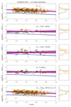 |
Fig. A.1. SFRFUV,corr vs. inclination for different UV-slope-related correction methods, as described in Appendix A. |
To build a statistically significant sample of galaxies in COSMOS at z ~ 0.7, we followed a standard assumption and assumed AV = 1. First, to judge whether assuming AV = 1 performs better than β at correcting the systematic SFRFUV/SFRMS offset, we have calculated SFRFUV,corr assuming AV = 1 for the 56 (28) galaxies with determined UV-slopes in the full (restricted) samples. We assumed the average Milky Way attenuation curve of Cardelli et al. (1989) and an RV = 3.1, resulting in an attenuation of 1 magnitude in the V band corresponding to a FUV attenuation of AFUV = 2.035 (or a y-intercept offset of ~ 1.2 dex). After correcting the galaxies with fitted β values by AFUV = 2.035, the best fits for the log(SFRFUV,corr/SFRMS)–inclination relation are  , and
, and  ) for the full sample and
  , and
, and  ) for the restricted sample. Interestingly, the slope has improved (SFRs have become more inclination independent) compared to no correction, and the y-intercept is also closer to zero. Compared to the β corrections from Boquien et al. (2012) used in Sect. 3.1, the slopes are consistent given the large uncertainties, and the y-intercept has not improved at all for the restricted sample, with SFRs remaining 0.12 ± 0.25 dex below the MS. However, the small sample size of galaxies with β still inhibits a robust comparison.
Applying the correction AV = 1 to all the galaxies in the COSMOS sample results in best-fit values of  , and
, and  ) for the full sample and
  , and
, and  ) for the restricted sample. As expected, the slope and scatter remain the same as for the uncorrected case, and the y-intercept becomes more consistent with zero. This indicates that using AFUV = 2.035 is an appropriate method for correcting the average dust attenuation for our sample of massive galaxies at z ~ 0.7, but a larger AFUV is required to bring the average SFR in line with the expected MS SFR for the full sample; a galaxy in the full sample or restricted sample with 1 − cos(i) = 0.5 lies 0.32 or 0.16 dex below the MS, respectively.
Combining the two approaches, we also fitted our samples adopting the UV-slope-derived attenuation where available and adopting AFUV = 2.035 where β was unavailable. Applying attenuation corrections based on the UV-slope or AV = 1 at z ~ 0.7 does not remove the inclination dependency of the SFRFUV: k1 = − 0.48 ± 0.12 and −0.47 ± 0.16 for the full and restricted samples, respectively. These results would suggest that applying AV = 1 performs similarly to the β–A FUV relation from Boquien et al. (2012) at z ~ 0.7, but larger samples of galaxies with well-determined UV-slopes would be required to confirm this. In addition, further corrections would still be required to remove the inclination dependence of the SFRs when applying a constant AFUV correction.
We found that Eq. (4) from Boquien et al. (2016) may not be appropriate for our sample of massive disc galaxies at z ~ 0.7 because the resulting SFRs lie below the expected MS, therefore we also tested the relation from Wang et al. (2016): (A.1)
(A.1)
Comparing rows 2 and 3 of Fig. A.1, it appears that the Wang et al. (2016) and Boquien et al. (2012) corrections perform similarly. The key difference is the increased scatter in the Wang et al. (2016) SFRs due to the stronger dependence on β. Further progress in determining the attenuation law for these galaxies at intermediate redshift could be made by (1) improving our measurements of β by using rest-frame UV spectra or more photometric observations, and (2) by increasing our sample size.
Appendix B: Different hybrid UV+MIR dust corrections at z ~ 0
Using different values for η in Eq. (4) or different monochromatic LTIR conversions will naturally result in different hybrid SFRFUV,corr values. In this section, we test MIR + UV hybrid methods that use the WISE 12 μm and WISE 22 μm fluxes to correct for FUV attenuation in our local samples.
We used the relation of Cluver et al. (2017, C17) to convert the W3 spectral luminosity into total-infrared luminosity (5–1100 μm): (B.1)
(B.1)
where L 12 is in units of solar luminosities. This relation was calibrated on the SINGS/KINGFISH sample (Dale et al. 2017) supplemented with several more luminous galaxies from the literature. Cluver et al. (2017) found a 1σ scatter of 0.15 dex in Eq. (B.1). Correcting the FUV luminosity using the Cluver et al. (2017) relation and Eq. (6) results in SFRFUV,corr that are systematically ~ 0.3 dex above the expected MS (see Table B.1) for both the restricted and full samples. This may indicate that 1) a lower value of η is required for our sample, 2) the Cluver et al. (2017) relation might give higher LTIR luminosities for our sample of galaxies because different WISE flux measurement methods were used in their study and ours, as well as a different definition of LIR, or 3) the adopted MS relation is ~ 0.1 dex too high at z ~ 0.07. If we had used the 22 μm (W4) data rather than the 12 μm (W3) fluxes to calculate LTIR, and the W4 calibration from Cluver et al. (2017), then our UV+MIR SFRs would be only slightly different, with a larger intrinsic scatter, as shown in Fig. B.1 and Table B.1. Cluver et al. (2017) also found a larger scatter in the W4–TIR relation (σ = 0.18 dex) than the W3–TIR relation (σ = 0.15). The uncertainty in the MS from using different SFR calibrations is about 0.1–0.2 dex, which is not sufficient to explain the 0.3 dex offset seen by the hybrid SFRs using the Cluver et al. (2017) relation for TIR luminosity. However, it is clear that the different assumptions that go in to calculating the monochromatic infrared luminosity and combining this with the FUV luminosity can alter the SFRs by ~ 0.3 dex.
Local SFRFUV,corr from the hybrid relations indicated in Fig. B.1.
 |
Fig. B.1. SFRFUV,corr vs. inclination for different MIR hybrid correction methods, as indicated in the panels. C17 refers to Cluver et al. (2017), W08 to Wuyts et al. (2008), and CT15 to Catalán-Torrecilla et al. (2015). |
We also tested hybrid SFRs using the Wuyts et al. (2008) SED (W08), following the methods used in L18 for both W3 (used in Sect. 6) and W4 fluxes. These methods give SFRs closer to the expected MS values, k2 = 0.15 and 0.14 for the 12 μm (W3) full and restricted samples, respectively, and k2 = 0.1 and 0.05 for the 22 μm (W4) full and restricted samples, respectively. However, the slope of the relation is still ~ −0.15 dex for the full sample. Wuyts et al. (2008) W4 correction on the restricted sample is the only hybrid example that shows a positive correlation between W4-corrected SFRs and inclination (k1 = 0.18 ± 0.1), but this is also the sub-sample with the fewest detected galaxies.
Rather than using a flux density to LIR conversion, Catalán-Torrecilla et al. (2015, CT15), gives the following prediction based on the energy balance approach: (B.2)
(B.2)
This correction results in SFRs similar to the W08 W4 hybrid SFRs. A galaxy in the full sample with inclination 1−cos(i) = 0.5 lies 0.025 dex above the MS. On the other hand, a galaxy in the restricted sample at 1 − cos(i) = 0.5 lies −0.05 dex below the MS. Catalán-Torrecilla et al. (2015) found a coefficient of ~ 4.5 (rather than 4.08 from the energy balance argument) when fitting to star-forming CALIFA galaxies, which would again increase the SFRs.
Figure A.1 shows that the different hybrid SFR methods are able to bring the FUV-SFRs of local galaxies into rough agreement with our best-fit MS and remove most of the inclination dependence. However, different calibrations can change the overall SFRFUV,corr by up to 0.2 dex. Table B.1 gives the best-fit values for the different hybrid correction methods discussed above. WISE band 4 is less sensitive than W3, so we have about half the number of galaxies in our samples when we use 22 μm corrections. Moreover, signal-to-noise ratio cuts were applied on SFRs and therefore depend on LTIR, explaining the different number of galaxies for our analysis using W08.
All Tables
Best-fit parameters of the relation log SFRFUV,corr/SFRMS(M⋆, z)) = k1(1 − cos(i)) + k2, where SFRFUV,corr is measured using three different methods.
All Figures
|
Fig. 1. Evaluating the inclination dependence of dust-corrected SFRFUV values. From top to bottom, the panels show the observed UV SFR, the SFR corrected based on the UV-slope, the hybrid MIR+UV determined SFR, and the SFR corrected based on the Tuffs et al. (2004) radiative transfer models as a function of inclination angle. Face-on galaxies are lie to the left, 1 − cos(i) ~ 0, and edge-on galaxies lie to the right, 1 − cos(i) ~ 1. The blue lines show the inclination relation for SFRFUV as observed with no dust corrections (top panel). The dust correction factors work to increase the SFRFUV and lessen the inclination dependence of the SFR. Fitted parameters are given in Table 1. Orange data points show the “restricted sample”, and the full sample is shown as a 2D density histogram. Magenta lines show 150 random realisations of linear parameters from our MCMC chain. Distributions of the y-axes, log(SFRFUV/SFRMS) are also displayed as histograms. The dotted line shows where the SFRFUV = SFRMS. |
| In the text | |
|
Fig. 2. UV-slope, β, distribution for restricted (orange) and full samples (grey) in our local sample (top panels) and z ~ 0.7 sample (bottom panels). |
| In the text | |
|
Fig. A.1. SFRFUV,corr vs. inclination for different UV-slope-related correction methods, as described in Appendix A. |
| In the text | |
|
Fig. B.1. SFRFUV,corr vs. inclination for different MIR hybrid correction methods, as indicated in the panels. C17 refers to Cluver et al. (2017), W08 to Wuyts et al. (2008), and CT15 to Catalán-Torrecilla et al. (2015). |
| In the text | |
Current usage metrics show cumulative count of Article Views (full-text article views including HTML views, PDF and ePub downloads, according to the available data) and Abstracts Views on Vision4Press platform.
Data correspond to usage on the plateform after 2015. The current usage metrics is available 48-96 hours after online publication and is updated daily on week days.
Initial download of the metrics may take a while.