| Issue |
A&A
Volume 616, August 2018
Gaia Data Release 2
|
|
|---|---|---|
| Article Number | A14 | |
| Number of page(s) | 15 | |
| Section | Celestial mechanics and astrometry | |
| DOI | https://doi.org/10.1051/0004-6361/201832916 | |
| Published online | 10 August 2018 | |
Gaia Data Release 2
The celestial reference frame (Gaia-CRF2)
1
Université Côte d’Azur,
Observatoire de la Côte d’Azur,
CNRS, Laboratoire Lagrange, Bd de l’Observatoire,
CS 34229,
06304 Nice Cedex 4,
France
2
Lohrmann Observatory,
Technische Universität Dresden,
Mommsenstraße 13,
01062 Dresden,
Germany
3
Lund Observatory, Department of Astronomy and Theoretical Physics, Lund University,
Box 43,
22100 Lund,
Sweden
4
European Space Astronomy Centre (ESA/ESAC),
Camino bajo del Castillo,
s/n,
Urbanizacion Villafranca del Castillo, Villanueva de la Cañada,
28692 Madrid,
Spain
5
Astronomisches Rechen-Institut,
Zentrum für Astronomie der Universität Heidelberg,
Mönchhofstr. 12-14,
69120 Heidelberg,
Germany
6
HE Space Operations BV for ESA/ESAC,
Camino bajo del Castillo,
s/n,
Urbanizacion Villafranca del Castillo, Villanueva de la Cañada,
28692 Madrid,
Spain
7
Vitrociset Belgium for ESA/ESAC,
Camino bajo del Castillo,
s/n,
Urbanizacion Villafranca del Castillo, Villanueva de la Cañada,
28692 Madrid,
Spain
8
ATG Europe for ESA/ESAC,
Camino bajo del Castillo,
s/n,
Urbanizacion Villafranca del Castillo, Villanueva de la Cañada,
28692 Madrid,
Spain
9
Telespazio Vega UK Ltd for ESA/ESAC,
Camino bajo del Castillo,
s/n,
Urbanizacion Villafranca del Castillo, Villanueva de la Cañada,
28692 Madrid,
Spain
10
GEPI,
Observatoire de Paris,
Université PSL,
CNRS,
5 Place Jules Janssen,
92190 Meudon,
France
11
Univ. Grenoble Alpes,
CNRS,
IPAG,
38000 Grenoble,
France
12
SYRTE,
Observatoire de Paris,
Université PSL,
CNRS, Sorbonne Université,
LNE,
61 avenue de l’Observatoire 75014 Paris,
France
13
ON/MCTI-BR,
Rua Gal. José Cristino 77,
Rio de Janeiro,
CEP 20921-400,
RJ,
Brazil
14
OV/UFRJ-BR,
Ladeira Pedro Antônio 43,
Rio de Janeiro,
CEP 20080-090,
RJ,
Brazil
15
Laboratoire d’astrophysique de Bordeaux,
Univ. Bordeaux,
CNRS,
B18N, allée Geoffroy Saint-Hilaire,
33615 Pessac,
France
16
Leiden Observatory, Leiden University,
Niels Bohrweg 2,
2333 CA Leiden,
The Netherlands
17
INAF - Osservatorio astronomico di Padova,
Vicolo Osservatorio 5,
35122 Padova,
Italy
18
Science Support Office,
Directorate of Science, European Space Research and Technology Centre (ESA/ESTEC),
Keplerlaan 1,
2201AZ,
Noordwijk,
The Netherlands
19
Max Planck Institute for Astronomy,
Königstuhl 17,
69117 Heidelberg,
Germany
20
Institute of Astronomy, University of Cambridge,
Madingley Road,
Cambridge CB3 0HA,
UK
21
Department of Astronomy, University of Geneva,
Chemin des Maillettes 51,
1290 Versoix,
Switzerland
22
Mission Operations Division, Operations Department,
Directorate of Science, European Space Research and Technology Centre (ESA/ESTEC),
Keplerlaan 1,
2201 AZ,
Noordwijk,
The Netherlands
23
Institut de Ciències del Cosmos,
Universitat de Barcelona (IEEC-UB),
Martí i Franquès 1,
08028 Barcelona,
Spain
24
CNES Centre Spatial de Toulouse,
18 avenue Edouard Belin,
31401 Toulouse Cedex 9,
France
25
Institut d’Astronomie et d’Astrophysique,
Université Libre de Bruxelles CP 226,
Boulevard du Triomphe,
1050 Brussels,
Belgium
26
F.R.S.-FNRS,
Rue d’Egmont 5,
1000 Brussels,
Belgium
27
INAF - Osservatorio Astrofisico di Arcetri,
Largo Enrico Fermi 5,
50125 Firenze,
Italy
28
Mullard Space Science Laboratory, University College London,
Holmbury St Mary,
Dorking,
Surrey RH5 6NT,
UK
29
INAF - Osservatorio Astrofisico di Torino,
via Osservatorio 20,
10025 Pino Torinese (TO),
Italy
30
INAF - Osservatorio di Astrofisica e Scienza dello Spazio di Bologna,
via Piero Gobetti 93/3,
40129 Bologna,
Italy
31
Serco Gestión de Negocios for ESA/ESAC,
Camino bajo del Castillo,
s/n,
Urbanizacion Villafranca del Castillo, Villanueva de la Cañada,
28692 Madrid,
Spain
32
ALTEC S.p.A,
Corso Marche,
79,
10146 Torino,
Italy
33
Department of Astronomy, University of Geneva,
Chemin d’Ecogia 16,
1290 Versoix,
Switzerland
34
Gaia DPAC Project Office,
ESAC,
Camino bajo del Castillo,
s/n, Urbanizacion Villafranca del Castillo,
Villanueva de la Cañada,
28692 Madrid,
Spain
35
National Observatory of Athens,
I. Metaxa and Vas. Pavlou,
Palaia Penteli,
15236 Athens,
Greece
36
IMCCE,
Observatoire de Paris,
Université PSL,
CNRS, Sorbonne Université,
Univ. Lille,
77 av. Denfert-Rochereau,
75014 Paris,
France
37
Royal Observatory of Belgium,
Ringlaan 3,
1180 Brussels,
Belgium
38
Institute for Astronomy, University of Edinburgh,
Royal Observatory,
Blackford Hill,
Edinburgh EH9 3HJ,
UK
39
Instituut voor Sterrenkunde,
KU Leuven,
Celestijnenlaan 200D,
3001 Leuven,
Belgium
40
Institut d’Astrophysique et de Géophysique,
Université de Liège,
19c,
Allée du 6 Août,
4000 Liège,
Belgium
41
Área de Lenguajes y Sistemas Informáticos, Universidad Pablo de Olavide,
Ctra. de Utrera,
km 1. 41013,
Sevilla,
Spain
42
ETSE Telecomunicación, Universidade de Vigo,
Campus Lagoas-Marcosende,
36310 Vigo,
Galicia,
Spain
43
Large Synoptic Survey Telescope,
950 N. Cherry Avenue,
Tucson,
AZ 85719,
USA
44
Observatoire Astronomique de Strasbourg,
Université de Strasbourg,
CNRS,
UMR 7550,
11 rue de l’Université,
67000 Strasbourg,
France
45
Kavli Institute for Cosmology, University of Cambridge,
Madingley Road,
Cambride CB3 0HA,
UK
46
Aurora Technology for ESA/ESAC,
Camino bajo del Castillo,
s/n,
Urbanizacion Villafranca del Castillo, Villanueva de la Cañada,
28692 Madrid,
Spain
47
Laboratoire Univers et Particules de Montpellier,
Université Montpellier,
Place Eugène Bataillon,
CC72,
34095 Montpellier Cedex 05,
France
48
Department of Physics and Astronomy,
Division of Astronomy and Space Physics, Uppsala University,
Box 516,
75120 Uppsala,
Sweden
49
CENTRA, Universidade de Lisboa,
FCUL,
Campo Grande,
Edif. C8,
1749-016 Lisboa,
Portugal
50
Università di Catania,
Dipartimento di Fisica e Astronomia,
Sezione Astrofisica,
Via S. Sofia 78,
95123 Catania,
Italy
51
INAF - Osservatorio Astrofisico di Catania,
via S. Sofia 78,
95123 Catania,
Italy
52
University of Vienna, Department of Astrophysics,
Türkenschanzstraße 17,
A1180 Vienna,
Austria
53
CITIC – Department of Computer Science, University of A Coruña,
Campus de Elviña s/n,
15071,
A Coruña,
Spain
54
CITIC – Astronomy and Astrophysics, University of A Coruña,
Campus de Elviña s/n,
15071,
A Coruña,
Spain
55
INAF - Osservatorio Astronomico di Roma,
Via di Frascati 33,
00078 Monte Porzio Catone (Roma),
Italy
56
Space Science Data Center - ASI,
Via del Politecnico SNC,
00133 Roma,
Italy
57
University of Helsinki, Department of Physics,
P.O. Box 64,
00014 Helsinki,
Finland
58
Finnish Geospatial Research Institute FGI,
Geodeetinrinne 2,
02430 Masala,
Finland
59
Isdefe for ESA/ESAC,
Camino bajo del Castillo,
s/n,
Urbanizacion Villafranca del Castillo, Villanueva de la Cañada,
28692 Madrid,
Spain
60
Institut UTINAM UMR6213,
CNRS,
OSU THETA Franche-Comté Bourgogne,
Université Bourgogne Franche-Comté,
25000 Besançon,
France
61
STFC,
Rutherford Appleton Laboratory,
Harwell,
Didcot,
OX11 0QX,
UK
62
Dpto. de Inteligencia Artificial,
UNED,
c/ Juan del Rosal 16,
28040 Madrid,
Spain
63
Elecnor Deimos Space for ESA/ESAC,
Camino bajo del Castillo,
s/n,
Urbanizacion Villafranca del Castillo, Villanueva de la Cañada,
28692 Madrid,
Spain
64
Thales Services for CNES Centre Spatial de Toulouse,
18 avenue Edouard Belin,
31401 Toulouse Cedex 9,
France
65
Department of Astrophysics/IMAPP, Radboud University,
P.O. Box 9010,
6500 GL Nijmegen,
The Netherlands
66
European Southern Observatory,
Karl-Schwarzschild-Str. 2,
85748 Garching,
Germany
67
Department of Terrestrial Magnetism,
Carnegie Institution for Science,
5241 Broad Branch Road,
NW,
Washington,
DC 20015-1305,
USA
68
Università di Torino,
Dipartimento di Fisica,
via Pietro Giuria 1,
10125 Torino,
Italy
69
Departamento de Astrofísica,
Centro de Astrobiología (CSIC-INTA),
ESA-ESAC. Camino Bajo del Castillo s/n. 28692 Villanueva de la Cañada,
Madrid,
Spain
70
Leicester Institute of Space and Earth Observation and Department of Physics and Astronomy, University of Leicester, University Road,
Leicester LE1 7RH,
UK
71
Departamento de Estadística, Universidad de Cádiz,
Calle República Árabe Saharawi s/n. 11510,
Puerto Real,
Cádiz,
Spain
72
Astronomical Institute Bern University,
Sidlerstrasse 5,
3012 Bern,
Switzerland (present address)
73
EURIX SRL,
Corso Vittorio Emanuele II 61,
10128,
Torino,
Italy
74
Harvard-Smithsonian Center for Astrophysics,
60 Garden Street,
Cambridge MA 02138,
USA
75
Kapteyn Astronomical Institute, University of Groningen,
Landleven 12,
9747 AD Groningen,
The Netherlands
76
SISSA - Scuola Internazionale Superiore di Studi Avanzati,
via Bonomea 265,
34136 Trieste,
Italy
77
University of Turin, Department of Computer Sciences,
Corso Svizzera 185,
10149 Torino,
Italy
78
SRON, Netherlands Institute for Space Research,
Sorbonnelaan 2,
3584CA,
Utrecht,
The Netherlands
79
Dpto. de Matemática Aplicada y Ciencias de la Computación,
Univ. de Cantabria,
ETS Ingenieros de Caminos,
Canales y Puertos, Avda. de los Castros s/n,
39005 Santander,
Spain
80
Unidad de Astronomía, Universidad de Antofagasta,
Avenida Angamos 601,
Antofagasta 1270300,
Chile
81
CRAAG - Centre de Recherche en Astronomie,
Astrophysique et Géophysique,
Route de l’Observatoire Bp 63 Bouzareah 16340 Algiers,
Algeria
82
University of Antwerp,
Onderzoeksgroep Toegepaste Wiskunde,
Middelheimlaan 1,
2020 Antwerp,
Belgium
83
INAF - Osservatorio Astronomico d’Abruzzo,
Via Mentore Maggini,
64100 Teramo,
Italy
84
Instituto de Astronomia,
Geofìsica e Ciências Atmosféricas, Universidade de São Paulo,
Rua do Matão,
1226, Cidade Universitaria,
05508-900 São Paulo,
SP,
Brazil
85
Departmentof Astrophysics,
Astronomy and Mechanics, National and Kapodistrian University of Athens,
Panepistimiopolis,
Zografos,
15783 Athens,
Greece
86
Leibniz Institute for Astrophysics Potsdam (AIP),
An der Sternwarte 16,
14482 Potsdam,
Germany
87
RHEA for ESA/ESAC,
Camino bajo del Castillo,
s/n,
Urbanizacion Villafranca del Castillo, Villanueva de la Cañada,
28692 Madrid,
Spain
88
ATOS for CNES Centre Spatial de Toulouse,
18 avenue Edouard Belin,
31401Toulouse Cedex 9,
France
89
School of Physics and Astronomy, Tel Aviv University,
Tel Aviv 6997801,
Israel
90
UNINOVA -CTS,
Campus FCT-UNL,
Monte da Caparica,
2829-516 Caparica,
Portugal
91
School of Physics,
O’Brien Centre for Science North, University College Dublin,
Belfield,
Dublin 4,
Ireland
92
Dipartimento di Fisica e Astronomia,
Università di Bologna,
Via Piero Gobetti 93/2,
40129 Bologna,
Italy
93
Barcelona Supercomputing Center - Centro Nacional de Supercomputación,
c/ Jordi Girona 29,
Ed. Nexus II,
08034 Barcelona,
Spain
94
Department of Computer Science, Electrical and Space Engineering, Luleå University of Technology,
Box 848,
S-981 28 Kiruna,
Sweden
95
Max Planck Institute for Extraterrestrial Physics,
High Energy Group,
Gießenbachstraße,
85741 Garching,
Germany
96
Astronomical Observatory Institute, Faculty of Physics, Adam Mickiewicz University,
Słoneczna 36,
60-286 Poznań,
Poland
97
Konkoly Observatory, Research Centre for Astronomy and Earth Sciences, Hungarian Academy of Sciences,
Konkoly Thege Miklós út 15-17,
1121 Budapest,
Hungary
98
Eötvös Loránd University,
Egyetem tér 1-3,
1053 Budapest,
Hungary
99
American Community Schools of Athens,
129 Aghias Paraskevis Ave. & Kazantzaki Street,
Halandri,
15234 Athens,
Greece
100
Faculty of Mathematics and Physics, University of Ljubljana,
Jadranska ulica 19,
1000 Ljubljana,
Slovenia
101
Villanova University, Department of Astrophysics and Planetary Science,
800 E Lancaster Avenue,
Villanova PA 19085,
USA
102
Physics Department, University of Antwerp,
Groenenborgerlaan 171,
2020 Antwerp,
Belgium
103
McWilliams Center for Cosmology, Department of Physics, Carnegie Mellon University,
5000 Forbes Avenue,
Pittsburgh,
PA 15213,
USA
104
Astronomical Institute, Academy of Sciences of the Czech Republic,
Fričova 298,
25165 Ondřejov,
Czech Republic
105
Telespazio for CNES Centre Spatial de Toulouse,
18 avenue Edouard Belin,
31401 Toulouse Cedex 9,
France
106
Institut de Physique de Rennes,
Université de Rennes 1,
35042 Rennes,
France
107
INAF - Osservatorio Astronomico di Capodimonte,
Via Moiariello 16,
80131,
Napoli,
Italy
108
Shanghai Astronomical Observatory, Chinese Academy of Sciences,
80 Nandan Rd,
200030 Shanghai,
China
109
School of Astronomy and Space Science, University of Chinese Academy of Sciences,
Beijing 100049,
China
110
Niels Bohr Institute, University of Copenhagen,
Juliane Maries Vej 30,
2100 Copenhagen Ø,
Denmark
111
DXC Technology,
Retortvej 8,
2500 Valby,
Denmark
112
Las Cumbres Observatory,
6740 Cortona Drive Suite 102,
Goleta,
CA 93117,
USA
113
Astrophysics Research Institute, Liverpool John Moores University,
146 Brownlow Hill,
Liverpool L3 5RF,
UK
114
Baja Observatory of University of Szeged,
Szegedi út III/70,
6500 Baja,
Hungary
115
Laboratoire AIM,
IRFU/Service d’Astrophysique - CEA/DSM - CNRS - Université Paris Diderot,
Bât 709,
CEA-Saclay,
91191 Gif-sur-Yvette Cedex,
France
116
Warsaw University Observatory,
Al. Ujazdowskie 4,
00-478 Warszawa,
Poland
117
Institute of Theoretical Physics, Faculty of Mathematics and Physics, Charles University in Prague,
Czech Republic
118
AKKA for CNES Centre Spatial de Toulouse,
18 avenue Edouard Belin,
31401 Toulouse Cedex 9,
France
119
HE Space Operations BV for ESA/ESTEC,
Keplerlaan 1,
2201AZ,
Noordwijk,
The Netherlands
120
Space Telescope Science Institute,
3700 San Martin Drive,
Baltimore,
MD 21218,
USA
121
QUASAR Science Resources for ESA/ESAC,
Camino bajo del Castillo,
s/n,
Urbanizacion Villafranca del Castillo, Villanueva de la Cañada,
28692 Madrid,
Spain
122
Fork Research,
Rua do Cruzado Osberno,
Lt. 1,
9 esq.,
Lisboa,
Portugal
123
APAVE SUDEUROPE SAS for CNES Centre Spatial de Toulouse,
18 avenue Edouard Belin,
31401 Toulouse Cedex 9,
France
124
Nordic Optical Telescope,
Rambla José Ana Fernández Pérez 7,
38711 Breña Baja,
Spain
125
Spanish Virtual Observatory,
Spain
126
Fundación Galileo Galilei - INAF,
Rambla José Ana Fernández Pérez 7,
38712 Breña Baja,
Santa Cruz de Tenerife,
Spain
127
INSA for ESA/ESAC,
Camino bajo del Castillo,
s/n,
Urbanizacion Villafranca del Castillo, Villanueva de la Cañada,
28692 Madrid,
Spain
128
Dpto. Arquitectura de Computadores y Automática,
Facultad de Informática, Universidad Complutense de Madrid,
C/ Prof. José García Santesmases s/n,
28040 Madrid,
Spain
129
H H Wills Physics Laboratory, University of Bristol,
Tyndall Avenue,
Bristol BS8 1TL,
UK
130
Institut d’Estudis Espacials de Catalunya (IEEC),
Gran Capita 2-4,
08034 Barcelona,
Spain
131
Applied Physics Department, Universidade de Vigo,
36310 Vigo,
Spain
132
Stellar Astrophysics Centre, Aarhus University, Department of Physics and Astronomy,
120 Ny Munkegade,
Building 1520,
8000 Aarhus C,
Denmark
133
Argelander-Institut für Astronomie,
Universität Bonn,
Auf dem Hügel 71,
53121 Bonn,
Germany
134
Research School of Astronomy and Astrophysics, Australian National University,
Canberra,
ACT 2611 Australia
135
Sorbonne Universités,
UPMC Univ. Paris 6 et CNRS,
UMR 7095,
Institut d’Astrophysique de Paris,
98 bis bd. Arago,
75014 Paris,
France
136
Department of Geosciences, Tel Aviv University,
Tel Aviv 6997801,
Israel
Received:
27
February
2018
Accepted:
16
April
2018
Abstract
Context. The second release of Gaia data (Gaia DR2) contains the astrometric parameters for more than half a million quasars. This set defines a kinematically non-rotating reference frame in the optical domain. A subset of these quasars have accurate VLBI positions that allow the axes of the reference frame to be aligned with the International Celestial Reference System (ICRF) radio frame.
Aims. We describe the astrometric and photometric properties of the quasars that were selected to represent the celestial reference frame of Gaia DR2 (Gaia-CRF2), and to compare the optical and radio positions for sources with accurate VLBI positions.
Methods. Descriptive statistics are used to characterise the overall properties of the quasar sample. Residual rotation and orientation errors and large-scale systematics are quantified by means of expansions in vector spherical harmonics. Positional differences are calculated relative to a prototype version of the forthcoming ICRF3.
Results. Gaia-CRF2 consists of the positions of a sample of 556 869 sources in Gaia DR2, obtained from a positional cross-match with the ICRF3-prototype and AllWISE AGN catalogues. The sample constitutes a clean, dense, and homogeneous set of extragalactic point sources in the magnitude range G ≃ 16 to 21 mag with accurately known optical positions. The median positional uncertainty is 0.12 mas for G < 18 mag and 0.5 mas at G = mag. Large-scale systematics are estimated to be in the range 20 to 30 μas. The accuracy claims are supported by the parallaxes and proper motions of the quasars in Gaia DR2. The optical positions for a subset of 2820 sources in common with the ICRF3-prototype show very good overall agreement with the radio positions, but several tens of sources have significantly discrepant positions.
Conclusions. Based on less than 40% of the data expected from the nominal Gaia mission, Gaia-CRF2 is the first realisation of a non-rotating global optical reference frame that meets the ICRS prescriptions, meaning that it is built only on extragalactic sources. Its accuracy matches the current radio frame of the ICRF, but the density of sources in all parts of the sky is much higher, except along the Galactic equator.
Key words: astrometry / reference systems / catalogs
Corresponding author: F. Mignard, e-mail: This email address is being protected from spambots. You need JavaScript enabled to view it.
© ESO 2018
1 Introduction
One of the key science objectives of the European Space Agency’s Gaia mission (Gaia Collaboration et al. 2016) is to build a rotation-free celestial reference frame in the visible wavelengths. This reference frame, which may be called the Gaia Celestial Reference Frame (Gaia-CRF), should meet the specifications of the International Celestial Reference System (ICRS; Arias et al. 1995) in that its axes are fixed with respect to distant extragalactic objects, that is, to quasars. For continuity with existing reference frames and consistency across the electromagnetic spectrum, the orientation of the axes should moreover coincide with the International Celestial Reference Frame (ICRF; Ma et al. 1998) that is established in the radio domain by means of VLBI observations of selected quasars.
The second release of data from Gaia (Gaia DR2; Gaia Collaboration 2018) provides complete astrometric data (positions, parallaxes, and proper motions) for more than 550 000 quasars. In the astrometric solution for Gaia DR2 (Lindegren 2018), subsets of these objects were used to avoid the rotation and align the axes with a prototype version of the forthcoming third realisation of the ICRF1. The purpose of this paper is to characterise the resulting reference frame, Gaia-CRF2, by analysing the astrometric and photometric properties of quasars that are identified in Gaia DR2 from a positional cross-match with existing catalogues, including the ICRF3-prototype.
Gaia-CRF2 is the first optical realisation of a reference frame at sub-milliarcsecond (mas) precision, using a large number of extragalactic objects. With a mean density of more than ten quasars per square degree, it represents a more than 100-fold increase in the number of objects from the current realisation at radio wavelengths, the ICRF2 (Fey et al. 2015). The Gaia-CRF2 is bound to replace the HIPPARCOS Celestial Reference Frame (HCRF) as the most accurate representation of the ICRS at optical wavelengths until the next release of Gaia data. While the positions of the generally faint quasars constitute the primary realisation of Gaia-CRF2, the positions and proper motions of the ≃1.3 billion stars in Gaia DR2 are nominally in the same reference frame and thus provide a secondary realisation that covers the magnitude range G ≃ 6 to 21 mag at similar precisions, which degrades with increasing distance from the reference epoch J2015.5. The properties of the stellar reference frame of Gaia DR2 are not discussed here.
This paper explains in Sect. 2 the selection of the Gaia sources from which we built the reference frame. Section 3 presents statistics summarising the overall properties of the reference frame in terms of the spatial distribution, accuracy, and magnitude distribution of the sources. The parallax and proper motion distributions are used as additional quality indicators and strengthen the confidence in the overall quality of the product. In Sect. 4 the optical positions in Gaia DR2 are compared with the VLBI frame realised in the ICRF3-prototype. A brief discussion of other quasars in the data release (Sect. 5) is followed by the conclusions in Sect. 6.
2 Construction of Gaia-CRF2
2.1 Principles
Starting with Gaia DR2, the astrometric processing of the Gaia data provides the parallax and the two proper motion components for most of the sources, in addition to the positions (see Lindegren 2018). As a consequence of the Gaia observing principle, the spin of the global reference frame must be constrained in some way in order to deliver stellar proper motions in a non-rotating frame. Less relevant for the underlying physics, but of great practical importance, is that the orientation of the resulting Gaia frame should coincide with the current best realisation of the ICRS in the radio domain as well as possible, as implemented by the ICRF2 and soon by the ICRF3.
These two objectives were achieved in the course of the iterated astrometric solution by analysing the provisional positions and proper motions of a pre-defined set of sources, and by adjusting the source and attitude parameters accordingly by means of the so-called frame rotator (Lindegren et al. 2012). Two types of sources were used for this purpose: a few thousand sources identified as the optical counterparts of ICRF sources were used to align the positions with the radio frame, and a much larger set of probable quasars found by a cross-match with existing quasar catalogues were used, together with the ICRF sources, to ensure that the set of quasar proper motions was globally non-rotating. The resulting solution is then a physical realisation of the Gaia frame that is rotationally stabilised on the quasars. The detailed procedure used for Gaia DR2 is described in Lindegren (2018).
2.2 Selection of quasars
Although Gaia is meant to be autonomous in terms of the recognition of quasars from their photometric properties (colours, variability), this functionality was not yet implemented for the first few releases. Therefore the sources that are currently identified as quasars are known objects drawn from available catalogues and cross-matched to Gaia sources by retaining the nearest positional match. In Gaia DR1, quasars where flagged from a compilation made before the mission (Andrei et al. 2014), and a subset of ICRF2 was used for the alignment. The heterogeneous spatial distribution of this compilation did not greatly affect the reference frame of Gaia DR1 because of the special procedures that were used to link it to the HCRF (Lindegren et al. 2016; Mignard et al. 2016).
For Gaia DR2, which is the first release that is completely independent of the earlier HIPPARCOS and Tycho catalogues, it was desirable to use the most recent VLBI positions for the orientation of the reference frame, and a large, homogeneous set of quasars for the rotation. The Gaia data were therefore cross-matched with two different sets of known quasars:
A prototype of the upcoming ICRF3, based on the VLBI solution of the Goddard Space Flight Center (GSFC) that comprises 4262 radio-loud quasars that are observed in the X (8.5 GHz) and S (2.3 GHz) bands. This catalogue, referred to here as the ICRF3-prototype, was kindly provided to the Gaia team by the IAU Working Group on ICRF3 (see Sect. 4) more than a year in advance of the scheduled release of the ICRF3. The positional accuracy is comparable to that of Gaia, and this set was used to align the reference frame of Gaia DR2 to the radio frame.
The all-sky sample of 1.4 million active galactic nuclei (AGNs) of Secrest et al. (2015), referred to below as the AllWISE AGN catalogue (AW in labels and captions). This catalogue resulted from observations by the Wide-field Infrared Survey Explorer (WISE; Wright et al. 2010) that operates in the mid-IR at 3.4, 4.6, 12, and 22 μm wavelength. The AllWISE AGN catalogue has a relatively homogenous sky coverage, except for the Galactic plane, where the coverage is less extensive because of Galactic extinction and confusion by stars, and at the ecliptic poles, which have a higher density because of the WISE scanning law. The sources are classified as AGNs from a two-colour infrared photometric criterion, and Secrest et al. (2015) estimated that the probability of stellar contamination is ≤ 4.0 × 10⁻⁵ per source. About half of the AllWISE AGN sources have an optical counterpart that is detected at least once by Gaia in its first two years.
Cross-matching the two catalogues with a provisional Gaia solution and applying some filters based on the Gaia astrometry (see Sect. 5.1, Eq.(13) in Lindegren 2018) resulted in a list of 492 007 putative quasars, including 2844 ICRF3-prototype objects. The filters select sources with good observation records, a parallax formal uncertainty < 1 mas, a reliable level of significance in parallax and proper motion, and they avoid the Galactic plane by imposing |sin b | > 0.1. These sources were used by the frame rotator, as explained above, when calculating the final solution; in Gaia DR2, they are identified by means of the flag frame_rotator_object_type. This subset of (presumed) quasars cannot, however, be regarded as a proper representation of Gaia-CRF2 because of the provisional nature of the solution used for the cross-matching and the relatively coarse selection criteria. Several of these sources were indeed later found to be Galactic stars.
A new selection of quasars was therefore made after Gaia DR2 was completed. This selection took advantage of the higher astrometric accuracy of Gaia DR2 and applied better selection criteria that are detailed in Sect. 5.2, Eq. (14), of Lindegren (2018). In particular, this updated selection takes the parallax zeropoint into account. This resulted in a set of 555 934 Gaia DR2 sources that are matched to the AllWISE AGN catalogue and 2820 sources that are matched to the ICRF3-prototype. The union of the two sets contains 556 869 Gaia DR2 sources. These sources and their positions in Gaia DR2 are a version of the Gaia-CRF that we call Gaia-CRF2.
The entire subsequent analysis in this paper (except in Sect. 5) is based on this sample or on subsets of it. For simplicity, we use the term quasar (QSO) for these objects, although other classifications (BL Lac object, Seyfert 1, etc.) may be more appropriate in many cases, and a very small number of them may be distant (> 1 kpc) Galactic stars.
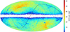 |
Fig. 1 Sky density per square degree for the quasars of Gaia-CRF2 on an equal-area Hammer–Aitoff projection in Galactic coordinates.The Galactic centre is at the origin of coordinates (centre of the map), Galactic north is up, and Galactic longitude increases from right to left. The solid black line shows the ecliptic. The higher density areas are located around the ecliptic poles. |
3 Properties of Gaia-CRF2
This sectiondescribes the overall astrometric and photometric properties in Gaia DR2 of the sources of the Gaia-CRF2, that is, the 556 869 quasars we obtained from the match to the AllWISE AGN catalogue and the ICRF3-prototype. Their sky density is displayed in Fig. 1. The Galactic plane area is filtered out by the AllWISE AGN selection criteria, while areas around the ecliptic poles are higher than the average density, as noted above. Lower density arcs from the WISE survey are also visible, but as a rule, the whole-sky coverage outside the Galactic plane has an average density of about 14 sources per deg2. The few sources in the Galactic plane area come from the ICRF3-prototype.
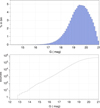 |
Fig. 2 G -magnitude distribution of the Gaia-CRF2 quasars. Percentage per bin of 0.1 mag (top) and cumulative distribution (bottom). |
3.1 Magnitude and colour
Figure 2 shows the magnitude distribution of the Gaia-CRF2 sources. In rounded numbers, there are 27 000 sources with G < 18 mag, 150 000 with G < 19 mag, and 400 000 with G < 20 mag. The average density of one source per square degree is reached at G = 18.2 mag, where it is likely that the sample is nearly complete outside the Galactic plane.
Figure 3 shows the distribution in colour index GBP− GRP (for the definition of the blue and red passbands, BP and RP, see Riello et al. 2018). Of the sources, 2154 (0.4%) have no colour index GBP− GRP in Gaia DR2. The distribution is rather narrow with a median of 0.71 mag and only 1% of the sources bluer than 0.28 mag or redder than 1.75 mag.
The magnitude is not evenly distributed on the sky, as shown in Fig. 4, with on the average fainter sources around the ecliptic poles, where the highest densities are found as well (Fig. 1). These two features result from a combination of the deeper survey of AllWISE in these areas and the more frequent Gaia observations from the scanning law.
3.2 Astrometric quality
In this section we describe the astrometric quality of the Gaia-CRF2 quasars based on the formal positional uncertainties and on the distribution of observed parallaxes and proper motions, which are not expected to be measurable by Gaia at the level of individual sources. We defer a direct comparison of the Gaia positions with VLBI astrometry to Sect. 4.
3.2.1 Formal uncertainty in position
As a single number characterising the positional uncertainty of a source, σpos,max, we take thesemi-major axis of the dispersion ellipse, computed from a combination σα* = σα cosδ, σδ, and the correlation coefficient ϱα,δ:
 (1)
(1)
Because this is also the highest eigenvalue of the 2 × 2 covariance matrix, it is invariant to a change of coordinates. These are formal uncertainties (see Sect. 3.2.2 for a discussion of how real they are) for the reference epoch J2015.5 of Gaia DR2. The results for the whole sample of Gaia-CRF2 quasars and the subset with G < 19 are shown in Fig. 5. The median accuracy is 0.40 mas for the full set and 0.20 mas for the brighter subset. Additional statistics are given in Table 1.
The main factors governing the positional accuracy are the magnitude (Fig. 6) and location on the sky (Fig. 7). The larger-than-average uncertainty along the ecliptic in Fig. 7 is conspicuous; this is a signature of the Gaia scanning law. This feature will also be present in future releases of Gaia astrometry and will remain an important characteristic of the Gaia-CRF.
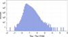 |
Fig. 3 Colour distribution of the Gaia-CRF2 quasars (log scale for the number of sources per bin of 0.1 mag). |
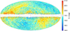 |
Fig. 4 Sky distribution of the Gaia-CRF2 source magnitudes. This map shows the median values of the G magnitude in cells of approximately 0.84 deg2 using an equal-area Hammer–Aitoff projection in Galactic coordinates. The Galactic centre is at the origin of coordinates (centre of the map), Galactic north is up, and Galactic longitude increases from right to left. |
3.2.2 Parallaxes and proper motions
Parallaxes and proper motions are nominally zero for the quasars that were selected for the reference frame (we neglect here the expected global pattern from the Galactic acceleration, which is expected to have an amplitude of 4.5 μas yr−1, see Sect. 3.3). Their statistics are useful as complementary indicators of the global quality of the frame and support the accuracy claim. Here we consider the global statistics before investigating possible systematics in Sect. 3.3. Figure 8 shows the distribution of the parallaxes for different magnitude-limited subsets. As explained in Lindegren (2018), the Gaia DR2 parallaxes have a global zeropoint error of − 0.029 mas, which is notcorrected for in the data available in the Gaia archive. This feature is well visible for the quasar sample and is a real instrumental effect that is not yet eliminated by the calibration models. Fortunately, the offset is similar for the different subsets. The shape of the distributions (best visible in the full set) is clearly non-Gaussian because of the mixture of normal distributions with a large spread in standard deviation, which is primarily linked to the source magnitude. The typical half-widths of the distributions (0.4, 0.3, and 0.2 mas) are of a similar size as the median positional uncertainties in Table 1.
The distribution of the normalised debiased parallaxes, computed as (ϖ +0.029 mas)∕σϖ, should follow a standard normal distribution (zero mean and unit variance) if the errors are Gaussian and the formal uncertainties σϖ are correctly estimated. The actual distribution for the full set of 556 869 quasars is plotted in Fig. 9. The red continuous curve is a normal distribution with zero mean and standard deviation 1.08; that this very closely follows the distribution up to normalised values of ± 3.5 is an amazing feature for real data. The magnitude effect is then fully absorbed by the normalisation, indicating that the Gaia accuracy in this brightness range is dominated by the photon noise. The factor 1.08 means that the formal uncertainties of the parallaxes are too small by 8%.
Similarly, the distributions in Fig. 10 for the normalised components of proper motions are very close to a normal distribution, with zero mean and standard deviations of 1.09 (μα*) and 1.11 (μδ). The extended distributions in log scale are very similar to the parallax and are not plotted.
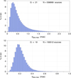 |
Fig. 5 Distribution of positional uncertainties σpos,max for the Gaia-CRF2 quasars: all sources (top) and G < 19 mag (bottom). |
Positional uncertainty σpos,max of the Gaia-CRF2 quasars.
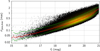 |
Fig. 6 Positional uncertainties σpos,max for the sources in the Gaia-CRF2 as function of the G magnitude. The red solid line is the running median, and the two green lines are the first and ninth decile. |
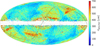 |
Fig. 7 Spatial distribution of the formal position uncertainty in Eq. (1) for the 407 959 sources of the Gaia-CRF2 with G < 20. The map shows the median value in each cell of approximately 0.84deg2, using a Hammer–Aitoff projection in Galactic coordinates with zero longitude at the centre and increasing longitude from right to left. The solid black line shows the ecliptic. |
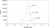 |
Fig. 8 Distribution of parallaxes in the Gaia archive for the Gaia-CRF2 quasars, subdivided by the maximum magnitude. The line at ϖ = −0.029 mas shows the global zeropoint offset. |
3.3 Systematic effects
3.3.1 Spatial distributions
In an ideal world, the errors in position, parallax, and proper motion should be purely random and not display any systematic patterns as function of position on the celestial sphere. While the non-uniform sampling of the sky produced by the Gaia scanning law is reflected in the formal uncertainties of the quasar astrometry, as shown in Fig. 7 for the positions, this does not imply that the errors (i.e. the deviations from the true values) show patterns of a similar nature. In the absence of a reliable external reference for the positions (except for the VLBI subset), the possibility of investigating the true errors in position is limited. However, the positions are derived from the same set of observations as the other astrometric parameters, using the same solution. Since the errors in parallax and proper motion are found to be in good agreement with the formal uncertainties calculated from the solution, we expect this to be the case for the positional errors as well.
Figure 11 shows maps in Galactic coordinates of the median parallax and proper motion components of the Gaia-CRF2 sources, calculated over cells of 4.669 deg2. For cells of this size, the median number of sources per cell is 70, with the exception of low Galactic latitude, where the density is lower (see Fig. 1), resulting in a larger scatter of the median from cell to cell than in other parts of the map. In Fig. 11 this is visible as an increased number of cells with red and blue colours, instead of green and yellow, in the less populated areas.
The median parallaxes shown in the top panel of Fig. 11 were corrected for the global zeropoint of − 29 μas (Sect. 3.2.2). In all three maps, various large-scale patterns are seen for Galactic latitudes |b| ≳ 10–15 deg, while at small angles (cell size), only a mixture of positive or negative offsets is visible that results from normal statistical scatter. The visual interpretation is complicated by large-scale patterns in the amplitude of the statistical scatter, in particular the smaller scatter in the second and fourth quadrants, that is, around the ecliptic poles. This is the result of a combination of the sky distribution of the sources (Fig. 1), their magnitudes (Fig. 4), and the Gaia scanning law (Fig. 7), which all exhibit similar patterns. Quantifying the large-scale systematics therefore requires a more detailed numerical analysis.
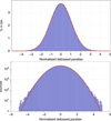 |
Fig. 9 Distribution of the normalised debiased parallaxes, (ϖ + 0.029 mas)∕σϖ, for the Gaia-CRF2 quasars in linear scale (top) and logarithmic (bottom). The red curve is a normal distribution with zero mean and standard deviation 1.08. |
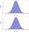 |
Fig. 10 Distributions of the normalised components of proper motions of the QSOs found with Gaia data, with μα* (top) and μδ (bottom) A normal distribution with zero mean and standard deviation of 1.09 for μα* (1.11 for μδ) is drawn in red. |
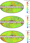 |
Fig. 11 Spatial distributions (in Galactic coordinates) of the parallaxes and proper motions of the Gaia-CRF2 quasars. From top to bottom: parallax (ϖ), proper motion in Galactic longitude (μl*), and proper motion in Galactic latitude (μb). Median values are computed in cells of approximately 5 deg2. Maps are in the Hammer–Aitoff projection with Galactic longitude zero at the centre and increasing from right to left. |
3.3.2 Spectral analysis
The vector field of the proper motions of the Gaia-CRF2 quasars was analysed using expansions on a set of vector spherical harmonics (VSH), as explained in Mignard & Klioner (2012) or Vityazev & Tsvetkov (2014).
In this approach the components of proper motion are projected onto a set of orthogonal functions up to a certain degree lmax. The terms of lower degrees provide global signatures such as the rotation and other important physical effects (secular acceleration, gravitational wave signatures), while harmonics of higher degree hold information on local distortions at different scales. Given the patternsseen in Fig. 11, we expect to see a slow decrease in the power of harmonics with l > 1. The harmonics of degree l = 1 play a special role, since any global rotation of the system of proper motions will be observed in the form of a rotation vector directly extracted from the three components with (l, m) = (1, 0), (1, −1), and (1, +1), where m is the order of the harmonic (|m|≤ l).
Mignard & Klioner (2012) derived a second global term from l = 1 that they called glide. This physically corresponds to a dipolar displacement originating at one point on a sphere and ending at the diametrically opposite point. For the quasar proper motions, this vector field is precisely the expected signature of the the galactocentric acceleration (Fanselow 1983; Bastian 1995; Sovers et al. 1998; Kovalevsky 2003; Titov & Lambert 2013). As summarised in Table 2, several VSH fits were made using different selections of quasars or other configuration parameters. Fit 1 uses all the quasars and fits only the rotation, without glide or harmonics with l > 1. This is very close to the conditions used to achieve the non-rotating frame in the astrometric solution for Gaia DR2. It is therefore not surprising that the rotation we find is much smaller than in the other experiments. The remaining rotation can be explained by differences in the set of sources used, treatment of outliers, and so on. This also illustrates the difficulty of producing a non-rotating frame that is non-rotating for every reasonable subset that a user may wish to select: This is not possible, at least at the level of formal uncertainties. Experiment 2 fits both the rotation and glide to all the data. The very small change in rotation compared with fit 1 shows the stability of the rotation resulting from the regular spatial distribution of the sources and the consequent near-orthogonality of the rotation and glide on this set. Fit 3 includes all harmonics of degree l ≤ 5, that is, 70 fitted parameters. Again the results do not change very much because of the good spatial distribution. The next five fits show the influence of the selection in magnitude and modulus of proper motion, and of not weighting the data by the inverse formal variance. In the next two fits (9a and 9b), the data are divided into two independent subsets, illustrating the statistical uncertainties. Most of these fits use fewer sources with a less regular distribution on the sky.
The last fit, fit 10, uses only the faint sources and has a similar glide but a very different rotation (x and y components, primarily), although it comprises the majority (73%) of the Gaia-CRF2 sources. This agrees with Figs. 3 and 4 in Lindegren (2018), which show a slight dependency on colour and magnitude of the Gaia spin relative to quasars. Again, this illustrates the sensitivity of the determination of the residual spin to the source selection, and at this stage, we cannot offer a better explanation than that a single solid rotation is too simple a model to fit the entire range of magnitudes. No attempt was made to introduce a magnitude equation in the fits.
The formal uncertainty of all the fits using at least a few hundred thousand quasars is of the order of 1 μas yr−1. It is tempting to conclude from this that the residual rotation of the frame with respect to the distant universe is of a similar magnitude. However, the scatter from one fit to the next is considerably larger, with some values exceeding 10 μas yr−1. Clearly, an overall solid rotation does not easily fit all the Gaia data, but gives results that vary with source selection well above the statistical noise. However, the degree of consistency between the various selections allows us to state that the residual rotation rate of the Gaia-CRF is probably not much higher than ± 10 μas yr−1 in each axis for any subset of sources.
The typical glide vector is about (−8, +5, +12) ± 1 μas yr−1 for the components in the ICRS. The expected signature for the galactocentric acceleration is a vector directed towards the Galactic centre with a magnitude of ≃4.50 μas yr−1, or (−0.25, −3.93, −2.18) μas yr−1 in the ICRScomponents. Clearly, the large-scale systematic effects in the Gaia proper motions, being of the order of 10 μas yr−1 at this stage of the data analysis, prevent a fruitful analysis of the quasar proper motion field in terms of the Galactic acceleration. For this purpose, an order-of-magnitude improvement is needed in the level of systematic errors, which may be achieved in future releases of Gaia data based on better instrument calibrations and a longer observation time-span. A similar improvement is needed to achieve the expected estimate of the energy flux of the primordial gravitational waves (Gwinn et al. 1997; Mignard & Klioner 2012; Klioner 2018).
The overall stability of the fits in Table 2 is partly due to the fairly uniform distribution of the Gaia-CRF2 sources over the celestial sphere, and it does not preclude the existence of significant large-scale distortions of the system of proper motions. Such systematics may be quantified by means of the fitted VSH, however, and a convenient synthetic indicator of how much signal is found at different angular scales is given by the total power in each degree l of the VSH expansion. This power  is invariant under orthogonal transformation (change of coordinate system) and therefore describes a more intrinsic, geometric feature than the individual components of the VSH expansion. The degree l corresponds to an angular scale of ~ 180°∕l.
In Fig. 12 (top panel) we plot  in μas yr−1, representing the RMS value of the vector field for the corresponding degree l. The lower panel in Fig. 12 shows the significance level of the power given as the equivalent standard normal variate derived from the asymptotic χ2 distribution; see Mignard & Klioner (2012) for details. The points labelled S and T correspond to the spheroidal and toroidal harmonics, with T&S for their quadratic combination. To illustrate the interpretation of the diagrams, for T1 the RMS value is
 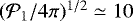 μas yr−1, which should be similar to the magnitude of the rotation vector for fit 3 in Table 2. The significance of this value is
  , corresponding to 7σ of a normal distribution, or a probability below 10−11.
For the low degrees plotted in Fig. 12, the power generally decreases with increasing l (smaller angular scales). This indicates that the systematics are generally dominated by the large angular scales. The total RMS for l ≤ 10 (angular scales ≳18 deg) is 42 μas yr−1.
Lindegren (2018) analysed the large-scale systematics of the Gaia DR2 proper motions of exactly the same quasar sample, using a very different spatial correlation technique. A characteristic angular scale of 20 deg was found, with an RMS amplitude of 28 μas yr−1 per component of proper motion (their Eq. (18)). Since this corresponds to 40 μas yr−1 for the total proper motion, their result is in good agreement with ours. They also found higher-amplitude oscillations with a spatial period of ≃1 deg, which in thepresent context of Gaia-CRF2 are almost indistinguishable from random noise, however.
Large-scale structure of the proper motion field of the Gaia-CRF2 quasars analysed using vector spherical harmonics.
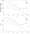 |
Fig. 12 Distributions of the RMS values (top) and their statistical levels of significance (bottom) in the VSH decomposition of the proper motion vector field of the Gaia-CRF2 from l = 1 to 10. S and T refer to the spheroidal and toroidal harmonics, and T&S signifies their quadratic combination. |
4 ICRF3-prototype subset of Gaia-CRF2
This sectiondescribes the subset of 2820 Gaia-CRF2 quasars matched to the ICRF3-prototype (Sect. 2.2), that is, the optical counterparts of compact radio sources with accurate VLBI positions. A comparison between the optical and VLBI positions is in fact a two-way exercise, as useful for understanding the radio frame as it is to Gaia, since neither of the two datasets is significantly better than the other. A similar investigation of the reference frame for Gaia DR1 (Mignard et al. 2016) showed the limitations of ICRF2, the currently available realisation of the ICRS, for such a comparison. A subset ICRF2 sources also had a less extensive VLBI observation record, the accuracy was lower for the best sources, and it would have been only marginally useful for a comparison to the Gaia DR2.
In discussions with the IAU working group in charge of preparing the upcoming ICRF3, which is scheduled for mid-2018, it was agreed that the working group would provide a prototype version of ICRF3 in the form of their best current solution to the Gaia team. This ICRF3-prototype was officially delivered in July 2017 and is particularly relevant in the current context for two reasons.
With the assumption that there is no globally systematic difference between the radio and optical positions, the commonsources allowed the axes of the two reference frames to be aligned, as explained in Lindegren (2018). The existence of radio–optical offsets with random orientation for each source is not a great problem for this purpose as it only adds white noise to the position differences. If large enough, it will be detected in the normalised position differences (Sect. 4.3).
The VLBI sources included in this prototype, together with the associated sets worked out in the X/Ka and K band (not yet released), are the most accurate global astrometric solutions available today that are fully independent of Gaia. The quoted uncertainties are very similar to what is formally achieved in Gaia DR2, and thebest-observed VLBI sources have positions that are nominally better than those from Gaia. This is therefore the only dataset from which the true errors and possible systematics in the positions of either dataset can be assessed and individual cases of truly discrepant positions between the radio and optical domains can be identified. The VLBI positions are less homogeneous in accuracy than the corresponding Gaia data, but the ≃1650 ICRF3-prototype sources with a (formal) position uncertainty <0.2 mas match the Gaia positions of the brighter (G < 18 mag) sources well in quality.
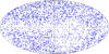 |
Fig. 13 Sky distribution of the 2820 Gaia sources identified as most probable optical counterparts of quasars in the ICRF3-prototype. Hammer–Aitoff projection in Galactic coordinates with origin at the centre of the map and longitude increasing from right to left. |
4.1 Properties of the Gaia sources in the ICRF3-prototype
Figure 13 shows the spatial distribution of the 2820 optical counterparts of ICRF3-prototype sources on the sky. The plot is in Galactic coordinates to facilitate comparison with Fig. 1, showing the full Gaia-CRF2 sample. The area in the lower right quadrant with low density corresponds to the region of the sky at δ < −40 deg with less VLBI coverage. Otherwise the distribution is relatively uniform, but with a slight depletion along the Galactic plane, as expected for an instrument operating at optical wavelengths.
The magnitude distribution of the ICRF3-prototype sources is shown in Fig. 14. The median is 18.8 mag, compared with 19.5 mag for the full Gaia-CRF2 sample shown in Fig. 2. The colour distribution (not shown) is similar to that of the full sample, shown in Fig. 2, only slightly redder: the median GBP − GRP is ≃ 0.8 mag for the ICRF3-prototype subset, compared with 0.7 mag for the full sample.
In terms of astrometric quality, the Gaia DR2 sources in the ICRF3-prototype subset do not differ significantly from other quasars in Gaia-CRF2 at the same magnitude. Figure 15 displays the formal uncertainty in position, computed with Eq. (1), as function of the G magnitude. Both the median relation and the scatter about the median are virtually the same as for the general population of quasars in Gaia-CRF2 shown in Fig. 6. For G ≳ 16.2, only few points in Fig. 15 lie clearly above the main relation. This may be linked to the change in the onboard CCD observation window allocation that occurs at G ≃ 16 (Gaia Collaboration et al. 2016). Four hundred and nine sources are brighter than G = 17.4, where the median position uncertainty as shown on Fig. 15 reaches 100 μas.
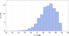 |
Fig. 14 Magnitude distribution of the 2820 Gaia sources identified as likely optical counterparts of quasars in the ICRF3-prototype. |
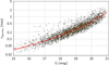 |
Fig. 15 Formal position uncertainty as a function of magnitude for the 2820 Gaia sources identified as optical counterparts of quasars in the ICRF3-prototype. The solid red line is a running median through the data points. |
4.2 Angular separations
We now compare the positions in Gaia DR2 and ICRF3-prototype directly for the 2820 quasars in common. Figure 16 gives in log-scale the distribution of the angular distances computed as
 (2)
(2)
where Δα* = (αGaia − αVLBI)cosδ. While for most of the sources, ρ is lower than 1 mas and very often much below this level, the number of discrepant sources is significant, and a few even have a position difference higher than 10 mas that would require individual examination.
To illustrate the dependence on the solution accuracies, Fig. 17 shows scatter plots of ρ versus the formal uncertainty in the ICRF3-prototype (top) and Gaia-CRF2 (bottom). Several of the most extreme distances in the top diagram are for sources with a large uncertainty in the ICRF3-prototype. However, some sources with nominally good solutions in both datasets exhibit large positional differences. These deserve more attention as the differences could represent real offsets between the centres of emission at optical and radio wavelengths. This is not further investigated in this paper, which is devoted to present the main properties of the Gaia-CRF2. Other explanations for the large differences can be put forward, such as a mismatch on the Gaia side when the optical counterpart is too faint and a distant star happens to be matched instead (unlikely at <10 mas distance); an extended galaxy around the quasar that is misinterpreted by the Gaia detector (should in general produce a poor solution); double or lensed quasars; or simply statistical outliers from the possibly extended tails of random errors. Although the ICRF3-prototype data in Fig. 17 cover a wider range in σpos,max than the Gaia data, the cores of both distributions extend from ≃ 0.1 to 0.5 mas.
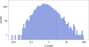 |
Fig. 16 Distribution of the angular separation ρ between Gaia DR2 and the ICRF3-prototype for the 2820 sources in common. Log-log scale plot with bins in ρ having a fractional width of 21∕5. |
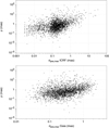 |
Fig. 17 Angular position differences ρ between Gaia DR2 and the ICRF3-prototype as function of the formal uncertainties σpos,max of the ICRF3-prototype (top) and Gaia DR2 (bottom). |
4.3 Normalised separations
The angular separations ρ become statistically more meaningful when scaled with the combined standard uncertainties. In the case of correlated variables, Mignard et al. (2016) have shown how to compute a dimensionless statistic X, called the normalised separation (their Eq. (4)). If the positional errors in both catalogues are Gaussian with the given covariances, then X is expected to follow a standard Rayleigh distribution, and values of X > 3 should be rare (probability ≃0.01). We caution that the normalisation used in this section depends on the reliability of the reported position uncertainties from the Gaia DR2 on one hand and from the ICRF3-prototype on the other hand. The latter are still provisional and purely formal, without noise floor and other overall adjustment, which will be introduced in the final release of the ICRF3.
Figure 18 is a scatter plot of ρ versus X, showing a fairly large subset of sources with X > 3 and even much larger. The most anomalous cases are found in the upper right part of the diagram. Some of the sources with the largest ρ are located in the upper centre of the diagram, with unremarkable X, meaning that their large angular separations are not significant in view of the formal uncertainties.
The diagram in Fig. 19 shows the frequency distribution of the normalised separations X with the standard Rayleigh probability density function superimposed as a solid red line. The frequency diagram includes all the sources, although 148 sources have a normalised separation > 10 and would be outside the frame. The distribution cannot be represented by a standard Rayleigh distribution, even though its mode is not very far from one, but the spread at large normalised separations is much too large. The departure from a pure Rayleigh distribution between VLBI positions and the Gaia DR1 has previously been noted in Petrov & Kovalev 2017 in a comparison using more than 6000 sources with VLBI positions. However, at this stage with the ICRF3-prototype, we cannot draw definite conclusions, and this issue will have to be reconsidered with the official release of ICRF3.
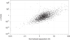 |
Fig. 18 Angular separation (ρ) vs. normalised separation (X) for the ICRF3-prototype subset of Gaia-CRF2. |
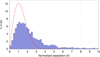 |
Fig. 19 Distribution of the normalised separations X between Gaia DR2 and the ICRF3-prototype. 148 sources have a normalised separation > 10. The red curves show the (standard) Rayleigh distributions for unit standard deviation. |
4.4 Large-scale systematics
In this section we analyse the positional difference between Gaia DR2 and the ICRF3-prototype in terms of large-scale spatial patterns. As in Sect. 3.3, the vector field of position differences is decomposed using VSH, where in particular the coefficients for degree l = 1 give the orientation difference of the two frames and a glide in position. Several fits were made to assess the stability of the orientation rotation against various selections of sources. Nominally, Gaia DR2 has been aligned to the ICRF3-prototype and no significant orientation difference should remain. However, stating that the two frames have been aligned is not the complete story, since the final alignment depends on many details of the fit: weighting scheme, outlier filtering, magnitude selection, and the model used for the fit. Furthermore, as explained in Sect. 2.2, the alignment was made using a slightly different set of ICRF3-prototype sources thancurrently considered. As a consequence of these differences, we often find statistically significant non-zero orientation errors in ourfits. The amplitude of these errors provides the best answer to the question of how precisely the two frames share the same axes.
The results of the various fits are summarised in Table 3. The first fit is similar to the alignment procedure in the astrometric solution for Gaia DR2 in that only the three orientation parameters (otherwise denoted ϵx, ϵy, ϵz) are fitted without a glide component. Of all the fits in the table, this has the overall smallest, statistically most insignificant orientation parameters. It gives a formal uncertainty in the alignment of about 30 μas per axis. Fit2, using the same data set, but fitting the glide as well, reveals a different picture. The orientation parameters remain negligible, but not as close to zero as in fit 1, and the glide components have a significant amplitude. The uncertainty is unchanged at about 30 μas. This is a good illustration of the ambiguity in the alignment when the procedure is not fully implemented.
In fits 3 to 5, only the orientation parameters are estimated, but with different filtering of the data, with or without statistical weighting of the differences. We showed in Sect. 4.1 that a subset of sources has good astrometric quality in both catalogues, but the position differences are not compatible with the formal uncertainties. Removing these sources from the fit greatly improves the formal precision of the fit, while the orientation parameters are changed by a few tens of μas, which is still only marginally significant. More significant changes result from including the glide and higher degrees of VSH (fits 6 to 8), or restricting the sample to the brighter subset (fits 9 and 10) with or without weighting. In these fits particularly the orientation error in x and the glide in y become significant. Finally, cases 11a and b are run on two independent halves of the data to ascertain the sensitivity of the solution to the selection.
Based on these experiments, we state that the axes of the Gaia-CRF2 and the ICRF3-prototype are aligned with an uncertainty of 20 to 30 μas, but no precise value can be provided without agreeing on the detailed model and numerical procedures for determining the orientation errors.
5 Other quasars in Gaia DR2
The cross-match of Gaia DR2 with the AllWISE AGN catalogue provided a very clean and homogeneous sample of quasars that is suitable for the definition of the Gaia-CRF2 and systematic investigation of its properties. However, other catalogues exist that will enlarge the sample of known or probable quasars in Gaia DR2 for other purposes. The Million Quasars Catalogue (MILLIQUAS; Flesch 2015) is a compilation of quasars and AGNs from the literature, including the release of SDSS-DR14 and AllWISE. We have cross-matched MILLIQUAS2 to Gaia DR2 using a matching radius of 5 arcsec, but otherwise applying the same selection criteria as for Gaia-CRF2. This yielded 1 007 920 sources with good five-parameter solutions in Gaia DR2, of which 501 204 are in common with the AllWISE selection in Gaia-CRF2.The magnitude distribution of the 506 716 additional sources is shown in Fig. 20. With a median G ≃ 20.2 mag, these sources are typically one magnitude fainter than the AllWISE AGNs in Gaia-CRF2, with positional uncertainties of about 1 mas.
Obviously, the Gaia DR2 release contains even more quasars. They can be found by cross-matching with other QSO catalogues such as the LQAC (Souchay et al. 2015) and various VLBI catalogues. Ultimately, a self-consistent identification of quasars from photometric and astrometric data of Gaia will be possible in a future release.
Global differences between the Gaia-CRF2 positions of ICRF sources and their positions in the ICRF3-prototype, expressed by the orientation and glide parameters.
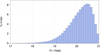 |
Fig. 20 Magnitude distribution for ~507 000 Gaia sources that are not included in Gaia-CRF2, but are tentatively identified as quasars through a cross-match with the MILLIQUAS catalogue. |
6 Conclusions
With Gaia DR2, a long-awaited promise of Gaia has come to fruition: the publication of the first full-fledged optical realisation of the ICRS, that is to say, an optical reference frame built only on extragalactic sources. Comprising more than half a million extragalactic sources that are globally positioned on the sky with a median uncertainty of 0.4 mas on average, this represents a major step in the history of non-rotating celestial reference frames built over the centuries by generations of astronomers. The brighter subset with G < 18 mag, comprising nearly 30 000 quasars with ≃0.12 mas astrometric accuracy, is the best reference frame available today and within relatively easy reach for telescopes of moderate size.
We have summarised the detailed content and mapped the main properties of Gaia-CRF2 as functions of magnitude and position. The quality claims regarding positional accuracy are supported by independent indicators such as the distribution of parallaxes or proper motions. Large-scale systematics are characterised by means of expansions in vector spherical harmonics. Comparison with VLBI positions in a prototype version of the forthcoming ICRF3 shows a globally satisfactory agreement at the level of 20 to 30 μas. Several sources with significant radio–optical differences of several mas require further investigation on a case-by-case basis.
Acknowledgements
This work has made use of data from the ESA space mission Gaia, processed by the Gaia Data Processing and Analysis Consortium (DPAC). We are grateful to the developers of TOPCAT (Taylor 2005) for their software. Funding for the DPAC has been provided by national institutions, in particular the institutions participating in the Gaia Multilateral Agreement. The Gaia mission website is http://www.cosmos.esa.int/gaia. The authors are members of the Gaia DPAC. This work has been supported by the European Space Agency in the framework of the Gaia project; the Centre National d’Etudes Spatiales (CNES); the French Centre National de la Recherche Scientifique (CNRS) and the Programme National GRAM of CNRS/INSU with INP and IN2P3 co-funded by CNES; the German Aerospace Agency DLR under grants 50QG0501, 50QG1401 50QG0601, 50QG0901, and 50QG1402; and the Swedish National Space Board. We gratefully acknowledge the IAU Working Group on ICRF3 for their cooperation during the preparation of this work and for their willingness to let us use an unpublished working version of the ICRF3 (solution from the GSFC).
References
- Andrei, H., Antón, S., Taris, F., et al. 2014, in Journées 2013 “Systèmes de référence spatio-temporels”, ed. N. Capitaine, 84 [Google Scholar]
- Arias, E. F., Charlot, P., Feissel, M., & Lestrade, J.-F. 1995, A&A, 303, 604 [NASA ADS] [Google Scholar]
- Bastian, U. 1995, in Future Possibilities for astrometry in Space, eds. M. A. C. Perryman, & F. van Leeuwen, ESA SP, 379, 99 [NASA ADS] [Google Scholar]
- Fanselow, J. L. 1983, Observation Model and parameter partial for the JPL VLBI parameter Estimation Software “MASTERFIT-V1.0”, Tech. Rep. [Google Scholar]
- Fey, A. L., Gordon, D., Jacobs, C. S., et al. 2015, AJ, 150, 58 [NASA ADS] [CrossRef] [Google Scholar]
- Flesch, E. W. 2015, PASA, 32, e010 [NASA ADS] [CrossRef] [Google Scholar]
- Gaia Collaboration (Prusti, T., et al.) 2016, A&A, 595, A1 [NASA ADS] [CrossRef] [EDP Sciences] [Google Scholar]
- Gaia Collaboration (Brown, A. G. A., et al.) 2018, A&A, 616, A1 (Gaia 2 SI) [NASA ADS] [CrossRef] [EDP Sciences] [Google Scholar]
- Gwinn, C. R., Eubanks, T. M., Pyne, T., Birkinshaw, M., & Matsakis, D. N. 1997, ApJ, 485, 87 [NASA ADS] [CrossRef] [Google Scholar]
- Klioner, S. A. 2018, Class. Quant. Grav., 35, 045005 [NASA ADS] [CrossRef] [Google Scholar]
- Klioner, S. A., & Soffel, M. 1998, A&A, 334, 1123 [NASA ADS] [Google Scholar]
- Kovalevsky, J. 2003, A&A, 404, 743 [NASA ADS] [CrossRef] [EDP Sciences] [Google Scholar]
- Lindegren, L., Lammers, U., Hobbs, D., et al. 2012, A&A, 538, A78 [NASA ADS] [CrossRef] [EDP Sciences] [Google Scholar]
- Lindegren, L., Lammers, U., Bastian, U., et al. 2016, A&A, 595, A4 [NASA ADS] [CrossRef] [EDP Sciences] [Google Scholar]
- Lindegren,, L., Hernández, J., Bombrun, A., et al. 2018, A&A, 616, A2 (Gaia 2 SI) [NASA ADS] [CrossRef] [EDP Sciences] [Google Scholar]
- Ma, C., Arias, E. F., Eubanks, T. M., et al. 1998, AJ, 116, 516 [NASA ADS] [CrossRef] [Google Scholar]
- Mignard, F., & Klioner, S. 2012, A&A, 547, A59 [NASA ADS] [CrossRef] [EDP Sciences] [Google Scholar]
- Mignard, F., Klioner, S., Lindegren, L., et al. 2016, A&A, 595, A5 [NASA ADS] [CrossRef] [EDP Sciences] [Google Scholar]
- Petrov, L., & Kovalev, Y. Y. 2017, MNRAS, 467, L71 [NASA ADS] [Google Scholar]
- Riello, M., De Angeli, F., Evans, D. W., et al. 2018, A&A, 616, A3 (Gaia 2 SI) [NASA ADS] [CrossRef] [EDP Sciences] [Google Scholar]
- Secrest, N. J., Dudik, R. P., Dorland, B. N., et al. 2015, ApJS, 221, 12 [NASA ADS] [CrossRef] [Google Scholar]
- Souchay, J., Andrei, A. H., Barache, C., et al. 2015, A&A, 583, A75 [NASA ADS] [CrossRef] [EDP Sciences] [Google Scholar]
- Sovers, O. J., Fanselow, J. L., & Jacobs, C. S. 1998, Rev. Mod. Phys., 70, 1393 [NASA ADS] [CrossRef] [Google Scholar]
- Taylor, M. B. 2005, in Astronomical Data Analysis Software and Systems XIV, eds. P. Shopbell, M. Britton, & R. Ebert, ASP Conf. Ser., 347, 29 [Google Scholar]
- Titov, O., & Lambert, S. 2013, A&A, 559, A95 [NASA ADS] [CrossRef] [EDP Sciences] [Google Scholar]
- Vityazev, V. V., & Tsvetkov, A. S. 2014, MNRAS, 442, 1249 [NASA ADS] [CrossRef] [Google Scholar]
- Wright, E. L., Eisenhardt, P. R. M., Mainzer, A. K., et al. 2010, AJ, 140, 1868 [NASA ADS] [CrossRef] [Google Scholar]
“Rotation” here refers exclusively to the kinematical rotation of the spatial axes of the barycentric celestial reference system (BCRS), as used in the Gaia catalogue, with respect to distant extragalactic objects (see e.g. Klioner & Soffel 1998). Similarly, “orientation” refers to the (non-) alignment of the axes at the reference epoch J2015.5.
http://quasars.org/milliquas.htm, version of August 2017, containing 1 998 464 entries.
All Tables
Large-scale structure of the proper motion field of the Gaia-CRF2 quasars analysed using vector spherical harmonics.
Global differences between the Gaia-CRF2 positions of ICRF sources and their positions in the ICRF3-prototype, expressed by the orientation and glide parameters.
All Figures
|
Fig. 1 Sky density per square degree for the quasars of Gaia-CRF2 on an equal-area Hammer–Aitoff projection in Galactic coordinates.The Galactic centre is at the origin of coordinates (centre of the map), Galactic north is up, and Galactic longitude increases from right to left. The solid black line shows the ecliptic. The higher density areas are located around the ecliptic poles. |
| In the text | |
|
Fig. 2 G -magnitude distribution of the Gaia-CRF2 quasars. Percentage per bin of 0.1 mag (top) and cumulative distribution (bottom). |
| In the text | |
|
Fig. 3 Colour distribution of the Gaia-CRF2 quasars (log scale for the number of sources per bin of 0.1 mag). |
| In the text | |
|
Fig. 4 Sky distribution of the Gaia-CRF2 source magnitudes. This map shows the median values of the G magnitude in cells of approximately 0.84 deg2 using an equal-area Hammer–Aitoff projection in Galactic coordinates. The Galactic centre is at the origin of coordinates (centre of the map), Galactic north is up, and Galactic longitude increases from right to left. |
| In the text | |
|
Fig. 5 Distribution of positional uncertainties σpos,max for the Gaia-CRF2 quasars: all sources (top) and G < 19 mag (bottom). |
| In the text | |
|
Fig. 6 Positional uncertainties σpos,max for the sources in the Gaia-CRF2 as function of the G magnitude. The red solid line is the running median, and the two green lines are the first and ninth decile. |
| In the text | |
|
Fig. 7 Spatial distribution of the formal position uncertainty in Eq. (1) for the 407 959 sources of the Gaia-CRF2 with G < 20. The map shows the median value in each cell of approximately 0.84deg2, using a Hammer–Aitoff projection in Galactic coordinates with zero longitude at the centre and increasing longitude from right to left. The solid black line shows the ecliptic. |
| In the text | |
|
Fig. 8 Distribution of parallaxes in the Gaia archive for the Gaia-CRF2 quasars, subdivided by the maximum magnitude. The line at ϖ = −0.029 mas shows the global zeropoint offset. |
| In the text | |
|
Fig. 9 Distribution of the normalised debiased parallaxes, (ϖ + 0.029 mas)∕σϖ, for the Gaia-CRF2 quasars in linear scale (top) and logarithmic (bottom). The red curve is a normal distribution with zero mean and standard deviation 1.08. |
| In the text | |
|
Fig. 10 Distributions of the normalised components of proper motions of the QSOs found with Gaia data, with μα* (top) and μδ (bottom) A normal distribution with zero mean and standard deviation of 1.09 for μα* (1.11 for μδ) is drawn in red. |
| In the text | |
|
Fig. 11 Spatial distributions (in Galactic coordinates) of the parallaxes and proper motions of the Gaia-CRF2 quasars. From top to bottom: parallax (ϖ), proper motion in Galactic longitude (μl*), and proper motion in Galactic latitude (μb). Median values are computed in cells of approximately 5 deg2. Maps are in the Hammer–Aitoff projection with Galactic longitude zero at the centre and increasing from right to left. |
| In the text | |
|
Fig. 12 Distributions of the RMS values (top) and their statistical levels of significance (bottom) in the VSH decomposition of the proper motion vector field of the Gaia-CRF2 from l = 1 to 10. S and T refer to the spheroidal and toroidal harmonics, and T&S signifies their quadratic combination. |
| In the text | |
|
Fig. 13 Sky distribution of the 2820 Gaia sources identified as most probable optical counterparts of quasars in the ICRF3-prototype. Hammer–Aitoff projection in Galactic coordinates with origin at the centre of the map and longitude increasing from right to left. |
| In the text | |
|
Fig. 14 Magnitude distribution of the 2820 Gaia sources identified as likely optical counterparts of quasars in the ICRF3-prototype. |
| In the text | |
|
Fig. 15 Formal position uncertainty as a function of magnitude for the 2820 Gaia sources identified as optical counterparts of quasars in the ICRF3-prototype. The solid red line is a running median through the data points. |
| In the text | |
|
Fig. 16 Distribution of the angular separation ρ between Gaia DR2 and the ICRF3-prototype for the 2820 sources in common. Log-log scale plot with bins in ρ having a fractional width of 21∕5. |
| In the text | |
|
Fig. 17 Angular position differences ρ between Gaia DR2 and the ICRF3-prototype as function of the formal uncertainties σpos,max of the ICRF3-prototype (top) and Gaia DR2 (bottom). |
| In the text | |
|
Fig. 18 Angular separation (ρ) vs. normalised separation (X) for the ICRF3-prototype subset of Gaia-CRF2. |
| In the text | |
|
Fig. 19 Distribution of the normalised separations X between Gaia DR2 and the ICRF3-prototype. 148 sources have a normalised separation > 10. The red curves show the (standard) Rayleigh distributions for unit standard deviation. |
| In the text | |
|
Fig. 20 Magnitude distribution for ~507 000 Gaia sources that are not included in Gaia-CRF2, but are tentatively identified as quasars through a cross-match with the MILLIQUAS catalogue. |
| In the text | |
Current usage metrics show cumulative count of Article Views (full-text article views including HTML views, PDF and ePub downloads, according to the available data) and Abstracts Views on Vision4Press platform.
Data correspond to usage on the plateform after 2015. The current usage metrics is available 48-96 hours after online publication and is updated daily on week days.
Initial download of the metrics may take a while.