| Issue |
A&A
Volume 616, August 2018
|
|
|---|---|---|
| Article Number | A54 | |
| Number of page(s) | 7 | |
| Section | Planets and planetary systems | |
| DOI | https://doi.org/10.1051/0004-6361/201832761 | |
| Published online | 15 August 2018 | |
Nucleus of active asteroid 358P/Pan-STARRS (P/2012 T1)
1
Max Planck Institute for Solar System Research,
Justus-von-Liebig-Weg 3,
37077
Göttingen,
Germany
e-mail: This email address is being protected from spambots. You need JavaScript enabled to view it.
2
Lowell Observatory,
1400 W Mars Hill Rd,
Flagstaff,
AZ 86001,
USA
3
Department of Physics and Astronomy, Northern Arizona University,
PO Box 6010,
Flagstaff,
AZ 86011,
USA
Received:
2
February
2018
Accepted:
17
May
2018
Abstract
Context. The dust emission from active asteroids is likely driven by collisions, fast rotation, sublimation of embedded ice, and combinations of these. Characterising these processes leads to a better understanding of their respective influence on the evolution of the asteroid population.
Aims. We study the role of fast rotation in the active asteroid 358P (P 2012/T1).
Methods. We obtained two nights of deep imaging of 358P with SOAR/Goodman and VLT/FORS2. We derived the rotational light curve from time-resolved photometry and searched for large fragments and debris >8 mm in a stacked, ultra-deep image.
Results. The nucleus has an absolute magnitude of mR = 19.68, corresponding to a diameter of 530 m for standard assumptions on the albedo and phase function of a C-type asteroid. We do not detect fragments or debris that would require fast rotation to reduce surface gravity to facilitate their escape. The 10-h light curve does not show an unambiguous periodicity.
Key words: minor planets / asteroids: individual: 358P
© ESO 2018
1 Introduction
Active asteroids have orbits typical of asteroids (with a Tisserand parameter relative to Jupiter >3; Kresák 1972), but temporarily display dust activity similar to comets (Hsieh & Jewitt 2006; Jewitt 2012; Jewitt et al. 2015b). While cometary activity is generally thought to be driven by the sublimation of embedded volatiles (Whipple 1950), the situation is likely more diverse in asteroids. Main belt asteroids have spent most of the time since their formation between the orbits of Mars and Jupiter, where solar heating prevents the persistence of near-surface ice over solar-system age timescales. But water ice can exist in the interiors of main belt asteroids if protected by a mantle of dust and debris (Schorghofer 2008; Prialnik & Rosenberg 2009; Capria et al. 2012).
Currently, five main belt asteroids are known to have ejected dust for extended periods of weeks to months during consecutive perihelion passages (Hsieh et al. 2004, 2015, 2011; Hsieh & Sheppard 2015; Jewitt et al. 2015a; Agarwal et al. 2017). This combination of protracted and recurrent activity is interpreted as a strong indication that the dust was lifted by gas-drag from sublimating ice (Hsieh et al. 2004). This subgroup of active asteroids is therefore also called the main belt comets (MBCs; Hsieh & Jewitt 2006). In some of the other active asteroids, the dust ejection has been an instantaneous process, such as an impact (Ishiguro et al. 2011a,b; Kim et al. 2017) or possibly break-up by fast rotation (Jewitt et al. 2013a; Hirabayashi & Scheeres 2014; Hirabayashi et al. 2014; Drahus et al. 2015). These same processes are also considered as the most likely triggers of sublimation-driven activity in MBCs by excavating ice from the interior (e.g. Haghighipour et al. 2016, 2018). Why sublimation is triggered in some objects and not in others may depend on the abundance and depth of ice, the magnitude of the excavating process, or both. Conversely, fast rotation can support the lifting of dust against gravity by a weak gas flow (Jewitt et al. 2014; Agarwal et al. 2016).
The active asteroid 358P (formerly designated P/2012 T1) was discovered in October 2012 by the Pan-STARRS1 survey (Chambers et al. 2016) owing to its bright cometary appearance (Wainscoat et al. 2012). 358P had passed perihelion at 2.41 AU on 10 September 2012, about one month before its discovery. The brightness of its dust coma first increased and then decreased over the following months, consistent with sublimation-driven activity (Hsieh et al. 2013). Numerical simulations reconstructing the production rate, size distribution, and ejection velocity of dust from the appearance of the dust tail indicate that the activity must have been ongoing for 3–5 months, starting at or one month before perihelion (Moreno et al. 2013). Spectroscopic searches for water vapour yielded an upper limit of 7.63 × 1025 molecules s−1 (O’Rourke et al. 2013; Snodgrass et al. 2017), which is still consistent with weak sublimation of water ice lifting the observed amount of dust.
We have observed 358P in July and August 2017, at true anomaly angles of 291° and 296°, prior to its return to perihelion in April 2018. The purpose of our observations was to (1) characterise the size, rotation and shape of the bare nucleus, which had been hidden in dust during all previous observations, and (2) to search for a debris trail and larger fragments along the orbit of 358P. The goal was to investigate whether fast rotation might be supporting ice sublimation in lifting the dust from 358P. We describe the observations and data analysis in Sect. 2. The results are presented in Sect. 3 and discussed in Sect. 4.
2 Observations and data processing
2.1 SOAR/Goodman
We observed 358P using the Goodman imaging spectrograph (Clemens et al. 2004) mounted on the Southern Astrophysical Research (SOAR) Telescope located on Cerro Pachón, Chile. Observations took place between 27 July 2017 UT 22:11 and 28 July 2017 UT 10:08; the observing geometry is described in Table 1. We used Goodman in imaging mode with 2 × 2 binning (0.3′′ pixel scale) and tracked the telescope at the rate of the target. We used integration times of 120 s (first 20 frames) and 150 s; background stars were trailed by l = 3′′ and l = 4′′, respectively. The goal of the observations was the recovery of the target (3σ positional uncertainty of the orbit at the time of observations: ~ 3′), the measurement of its rotational period using the broadband V R filter (centred at 610 nm with full width at half maximum – FWHM – of 200 nm), and the measurement of its optical colours using Sloan g, r, and i filters to put constraints on its taxonomic classification. Our observations were compromised by highly variable transparency conditions and cloud coverage, allowing for useful observations over only about 2 h out of 9 h. Furthermore, the target turned out to be significantly fainter than the brightness predicted by the JPL Horizons system (Giorgini et al. 1996). We were able to recover the target (Mommert et al. 2017) and extract a partial light curve from our VR observations. The g, r, and i filter observations were excluded from further analysis because of their marginal S/N.
The image data were corrected using bias and dome flat-field images taken on the same night. Astrometry and instrumental aperture photometry were derived from the VR images taken during the clear portion of the night using the PHOTOMETRYPIPELINE (PP; Mommert 2017). The PP provides automated astrometric and photometric analysis for imaging data and has been specifically designed for moving target observations. We photometrically calibrated our observations against Cousins R-band transformed from Pan-STARRS DR1 r magnitudes (Tonry et al. 2012; Flewelling et al. 2016), using no less than five background stars with solar-like colours (0.24 ≤ g − r ≤ 0.64 and − 0.09 ≤ r − i ≤ 0.31 in Sloan gri) in order to minimise systematic effects caused by the use of the V R filter while calibrating against R. Because of the highly variable seeing conditions, we adopted variable apertures for both 358P and the background stars; the full width at half maximum (FWHMbg) of the background stars varies between 0.5′′ and 1.5′′ over the transparent part of the night. We used aperture radii of r = 1.3 × FWHMbg for 358P, and of r = l/2 + 1.3 × FWHMbg for stars. In order to mitigate effects caused by the different aperture sizes, we applied empirical magnitude offsets to the target photometry in such a way as to keep the flux level of five bright stars constant; these corrections are significantly smaller than the typical photometric uncertainties of the target. The measured photometry from our SOAR observations, which is subject to significant noise, is plotted in the top panel of Fig. 1. The weighted average brightness of the target from this partial light curve is mR = 23.84 ± 0.11.
Journal of our observations of 358P.
2.2 VLT/FORS2
We also observed 358P for 10 h beginning on 17 August 2018 UT 23:37, using the FOcal Reducer and low dispersion Spectrograph 2 (FORS2; Appenzeller et al. 1998) mounted on the Unit 1 telescope (UT1) of the European Southern Observatory’s (ESO) Very Large Telescope (VLT) on Cerro Paranal in Chile. We obtained 77 images with an exposure time of 400 s in the R_SPECIAL+76 filter (central wavelength 655 nm, bandwidth 165.0 nm) in 2 × 2 binning mode, corresponding to a linear pixel scale of 0.25′′. The sky conditions were clear, possibly photometric. The geometry and distance at the time of observation are listed in Table 1.
The images were bias-subtracted and flatfielded using the Esorex pipeline, version 3.11.1 (Freudling et al. 2013). We derived the temporal variation of the seeing from profiles of 22 field stars not saturating the CCD detector. Stars were trailed by l = 13.67 pixels because the telescope was tracking the non-siderial motion of 358P, and the trails were inclined by 29° relative to the image x-axis. We fitted brightness profiles measured parallel to the y-axis with a Gaussian function, and used its FWHM, D, as a proxy of that of the seeing disc. The quantity D varied between 3 and 6 pixels (0.75′′ and 1.5′′) over the course of the night.
The data analysis procedure used for the VLT data is very similar to that used for our SOAR observations. Using PP, we performed aperture photometry on background stars using an aperture radius of r = l/2 + 1.3D and derivedthe magnitude zeropoint for each frame calibrated against Pan-STARRS DR1 r photometry transformed to Cousins R, requiring a minimum of three non-saturated background stars with solar-like colours. Target aperture photometry was obtained using a variable aperture with radius r = 1.3D (Fig. 1, bottom). We applied empirical magnitude offsets to the target photometry in such a way as to keep the flux level of ten bright stars constant; these corrections are significantly smaller than the typical photometric uncertainties of the target. To account for the systematic loss of flux due to the small aperture, we corrected the measured magnitudes by subtracting 0.09 (Sect. 3.2). The weighted average brightness of the target derived from all VLT data points shown in Fig. 1 is mR = 23.46 ± 0.01.
Figure 2 shows the measured apparent magnitude as a function of the measured FWHM of the seeing, which is proportional to the employed aperture radius. The Pearson correlation coefficient between the corresponding flux and the FWHM is R = 0.17, indicating a weak correlation between the measured flux and employed aperture size.
 |
Fig. 1 Light curve of 358P on 28 July 2017 observed with SOAR/Goodman (top panel) and on 18 August 2017 observed with VLT/FORS2 (bottom panel). The flux was measured in apertures of radius 1.3D, and for the VLT data set corrected by an offset of –0.09 mag to account for the loss of flux due to the small aperture. This correction was not applied for the SOARdata set because the FWHM was measured as average over the moderately trailed stars. The loss of flux due to the small aperture was therefore less than in the FORS data. The correction would have been small compared to the large scatter and error bars of the data. Open symbols in the bottom panel indicate data obtained after UT 8:00 for comparison with Fig. 2. The scale on the right-hand side vertical axes indicates the derived absolute magnitude according to Eq. (1) and for G = 0.15. The shaded areas in both panels indicate the range of absolute magnitudes covered by the VLT data. |
3 Results
3.1 Light curve
To assess the rotational properties of 358P, we concentrate on the VLT data, which have a longer time coverage than the SOAR data and smaller photometric uncertainties. Using an implementation of the Lomb–Scargle periodogram provided by astropy (Astropy Collaboration et al. 2013), we investigate periodicity in the brightness variations plotted in Fig. 1 (bottom). Since the amplitude of the variation is of the order of a few 0.1 mag, which is only slightly higher than the typical photometricuncertainty, we take a statistical approach. We account for the photometric uncertainties, by varying the measured brightness in each frame in a Gaussian way, according to the derived uncertainties. We apply the Lomb–Scargle algorithm to this randomised data set and derive the power-frequency distribution for potential light curve periods between 1 and 10 h (the duration of the observations). By repeating this method for 1000 randomised data sets and summing upthe individual power-frequency distributions, we obtain a distribution that accounts for the significant photometricuncertainties in the data. Because of the unknown complexity of the rotational light curve (Fourier order n), we repeat this analysis for a range of Fourier orders (1 ≤ n ≤ 5).
The resulting spectral power distributions are shown in Fig. 3. Relative power maxima independent of the Fourier order n appear at approximately 2 and 4 h. For n >1, additional power maxima appear in between, all of which have comparable strength. The 4 h periodicity, which would indicate an 8 h rotation period for a double-peaked light curve, agrees with the light curve behaviour observed during the first 8 h of our VLT/FORS2 observations (filled symbols in Figs.1 and 2). Data from the last 2 h (open symbols in Figs. 1 and 2) were obtained under deterioratedseeing conditions and may be less reliable. From Fig. 3 we are unable to derive an unambiguous rotational period for 358P. Potential explanations are that the object is rather spherical or observed from a polar perspective, leading to a light curve amplitude that is smaller than our photometric uncertatinties, or that the object’s rotational period is significantly longer than 10 h. We discuss this result in detail in Sect. 4.
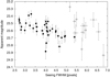 |
Fig. 2 Measured magnitude from VLT data as a function of the seeing FWHM, which is proportional to the aperture radius. The two quantities show a weak degree of statistical dependence (R = 0.17). Open symbols indicate data points obtained after UT 8:00 (see Fig. 1.) |
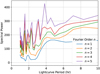 |
Fig. 3 Spectral power distributions for the light curve period (which corresponds to half the rotation period for a shape-induced double-peaked light curve) of 358P using a statistical approach. For any period in the range, the distributions provide the spectral power as derived with a Lomb–Scargle algorithm; the coloured lines denote different Fourier orders. We are unable to identify a clear periodicity in the period range that was probed. |
3.2 Radial profile and dust coma
To search for dust near the nucleus in the FORS2 images, we compared radial flux profiles of 358P with those of field stars. Since stars were trailed in the exposures targeting 358P, we used two calibration exposures of standard star fields obtained at siderial tracking at the beginning and end of the night, respectively, to measure the stellar radial profiles. We averaged the normalised profiles of 14 and 26 non-saturated field stars, respectively. For comparison, we selected exposures of 358P obtained under similar seeing conditions (as indicated by the FITS header keyword FWHMLINOBS). The keyword FWHMLINOBS seems to have generic values for the first 21 frames of the data, which we consider unreliable. For the remaining 56 frames, the values of FWHMLINOBS and our measured D are well correlated with a Pearson correlation coefficient of 0.88. The frames we used for comparison to the standard star fields are from this second part of the data set. We used a single 358P exposure (frame 40) for comparison with the first standard star field, and six exposures (frames 70 + 73–77) for the second star field that we averaged in the co-moving frame. Figure 4 shows the resulting radial profiles. For both values of the seeing parameter D, the profiles of 358P and the stars are similar, and they are also similar for different seeing conditions if expressed in units of D. The radial profile of 358P is consistent with that of a point source. It does not show evidence of broadening by dust. Figure 4 shows that the percentage of flux enclosed in a given multiple of D is independent of the value of D. At a radius of 1.3D, the aperture encloses 92% of the total flux, requiring a magnitude correction of Δ M = –0.09 (cf. Fig. 1).
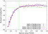 |
Fig. 4 Normalised radial profiles of 358P and field stars in the FORS2 data, measured for two different values of the seeing FWHM, D. The green lines indicate the aperture radius in which the light curve (Fig. 1) was measured and the corresponding flux level of 92%. The x-axis is in units of the FWHM at observation, i.e. a unit interval corresponds to 3.4 pixels for the blue dots and 5.4 pixels for the red dots. |
3.3 Nucleus size
We constrain the size of the nucleus from the VLT/FORS2 observations only, since they cover a longer fraction of the target’s light curve and we assume these observations provide a better approximation of its mean brightness than the SOAR/Goodman observations. The absolute magnitude, HR (corresponding to rh = Δ = 1 AU and α = 0) is given by
 (1)
(1)
where Φ(α) is the phase function describing the ratio of the scattered light at phase angle α to that at α = 0°. We used the HG approximation of Φ(α) with G = 0.15 corresponding to C-type asteroids (Bowell et al. 1989). The measured apparent magnitude of mR = 23.46 ± 0.01 (Sect. 2.2) corresponds to an absolute magnitude of HR = 19.68 ± 0.01. Assuming an S-type phase function with G = 0.25 would result in HR = 19.74 ± 0.01 instead. The absolute magnitude derived from the average brightness in the SOAR/Goodman data (mR = 23.84 ± 0.11) is HR = 19.84 ± 0.11 (G = 0.15) or HR = 19.91 ± 0.11 (G = 0.25). Since the stated uncertainties of the mean correspond to 1σ, the two measurements are marginally consistent.
We base our following estimate of the nucleus size on the value HR = 19.68 ± 0.01 measured from the VLT data and assuming a C-type phase function. For a geometric albedo of pV = 0.06 (we approximate pR with pV, which is reasonably close for low albedos) typical for C-type asteroids (Nugent et al. 2016), the absolute magnitude corresponds to an equivalent-sphere radius of
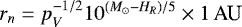 (2)
(2)
(e.g. Harris & Lagerros 2002). For a solar magnitude of M⊙ = −27.15 in Cousins R-band (Binney & Merrifield 1998), we obtain rn = 263 m. The main source of uncertainty is the unknown albedo of 358P. The C-type albedos given in Nugent et al. (2016) vary within a factor of 3, which leads to a radius uncertainty of a factor 1.7. The unknown phase function, by contrast, induces only a small uncertainty due to the low phase angle at the time of observation. The radius derived for G = 0.25 would only be 3% smaller than for G = 0.15. The radius uncertainty introduced by the photometric uncertainty is also 3%. The escape speed from the surface of a non-rotating body of sub-km size and assuming a density of ρ = 1500 kg m−3 (Hanuš et al. 2017) is vesc = 0.2 m s−1. The densityreported by Hanuš et al. (2017) was measured for C-type asteroids >100 km in diameter.We use this value for the much smaller 358P owing to the lack of measurements for a C-type object of this size. An asteroid with known density and comparable in size to 358P is the S-type (25143) Itokawa. Its density ρ = 1900 kg m−3 (Fujiwara et al. 2006) is near the lower end of the interval of (2000–4000) kg m−3 observed for S-types by Hanuš et al. (2017), which is a result of Itokawa’s high macroporosity and rubble-pile nature (Fujiwara et al. 2006).
3.4 Upper limits for trail brightness and fragment size
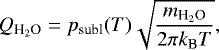
We searchedfor a faint dust trail in a deep composite image of all 77 FORS2 exposures. To obtain the composite, we first scaled each background-subtracted exposure, i, with a factor fi = 100.4ΔMi to compensate for the variable atmospheric extinction, where ΔMi is the offset of the averaged instrumental magnitude of a set of field stars from an (arbitrary) reference magnitude. Subsequently, we averaged all frames in the siderial reference frame rejecting the faintest and the three brightest values at each position, and subtracted the resulting stellar composite from each exposure. Finally, we averaged all frames in the co-moving frame of 358P with the same rejection rule. Figures 5 and 6 show the resulting deep image of 358P.
To derive an upper limit for the surface brightness of the debris trail, we assume that an extended linear object having S∕N = 1 per pixel is easily detectable to the human eye (Agarwal et al. 2010), and that the trail surface brightness must therefore be smaller than the local standard deviation of the background flux, σ = 20 ADU, in the composite image (Fig. 5). This corresponds to an upper limit on the surface brightness of 28.4 mag arcsec−2 in Cousins R, which is three magnitudes fainter than the surface brightness of the debris trails of the active asteroids P/2010 A2 (Jewitt et al. 2013b) and 331P (Drahus et al. 2015).
We proceed to infer an upper limit on the size of individual large fragments assuming that point sources with S∕N > 3 would be detectable. Following Makovoz & Marleau (2005), we use  , where f is the total flux from the point source and r is the radius of theaperture. For r = 4 pixels, we find that f > 425 ADU is required, corresponding to a limiting apparent magnitude of 27.8 in Cousins R-band. At the position of 358P during our VLT/FORS2 observations, this corresponds to an absolute magnitude of 24.0 (Eq. (1)) or a diameter of 72 m (Eq. (2)).
 |
Fig. 5 358P in a composite of 77 FORS2 exposures, averaged in the co-moving frame of the asteroid. The brightness scale is inverted and linear, and the arrows indicate the anti-solar direction and the projected negative orbital velocity vector. No indication of a debris trail (which should be parallel to the negative velocity vector) is visible. |
 |
Fig. 6 Zoom-in on Fig. 5. The brightness scale is inverted and logarithmic, and the size of the image is 35′′ × 21′′. |
3.5 Production of cm-sized debris
Whether a particle ejected in 2012 remains in the FOV of our 2017 observation depends on its velocity component, ve, parallel to the orbital motion of 358P upon decoupling from its gravitational influence (Müller et al. 2001), and on the ratio of solar radiation pressure to local solar gravity, β = 5.77 × 10⁻⁴Qpr∕(ρa), where a and ρ are the radius and bulk density of the particle and the dimensionless parameter Qpr characterises the optical properties of the material (Burns et al. 1979). We numerically simulated the motion of test particles ejected during the 2012 perihelion passage that have a wide range of values for β and ve, and calculated their positions relative to 358P at the time of our FORS2 observation in August 2017. Only particles that have
 (3)
(3)
would still be in the FOV of our observations, where vb = −ve is positive towards the direction opposite to the orbital motion of 358P. Particles ejected to this direction stay closer to the nucleus than particles ejected to the forward direction at the same relative speed because backward ejection decreases the orbital energy and period of the particle, counteracting radiation pressure. The hatched blue area in Fig. 7 shows possible backward ejection speeds as a function of particle size.
In the following, we derive the maximum particle speed consistent with the measured upper limit of the water production rate Qmax = 7.63 × 1025 molecules s−1 (O’Rourke et al. 2013), assuming that the activity was confined to a patch on the surface. The temperature of a sublimating surface containing water ice at the heliocentric distance rh is given from the equilibrium of solar irradiation with cooling by radiation and sublimation,
 (4)
(4)
where ϵ and AB are the emissivity and Bond albedo of the surface, σ and NA the Stefan–Boltzmann and Avogadro constants, L = 51 000 J mol−1 the latent heat of water ice,  the molecular mass of water, and θ the angle between the surface normal and solar direction. The value
  is the sublimation rate of water ice in vacuum in kg s−1 m−2 given by
 (5)
(5)
where the sublimation pressure is given by psubl(T) = Aexp(−B∕T) with A = 3.56 × 10¹² Pa and B = 6141 K (Fanale & Salvail 1984).
Assuming extreme values of ϵ = 1, AB = 0 and normal incidence (θ = 0), we obtain an upper limit for the temperature Tmax = 191 K at the perihelion distance of 358P (rh = 2.41 AU), and a sublimation rate of  = 1.74 × 10²¹ molecules s−1 m−2. Assuming that the activity was confined to a circular patch on the surface, and that this patch was not illuminated and inactive for 50% of each diurnal cycle, the observational upper limit Qmax translates to a maximum patch radius of 170 m, or 10% of the surface.
From a patch of this size, assuming a bulk density of 1500 kg m−3 for both dust and nucleus and a unit gas drag coefficient, the maximum escaping grain size would be 5 cm (Eq. (A6) in Jewitt et al. 2014; cf. Fig. 7). The maximum liftable grain radius scales about linearly with the patch radius. Assuming instead a comet-like density of 500 kg m−3 for both dust and nucleus would increase the maximum liftable grain radius to ~35 cm.
The sizeand velocity ranges compatible with both the gas production and dynamical constraint (overlapping red and hatched areas in Fig. 7) are consistent with the velocity-size relation used by Moreno et al. (2013), that is
 (6)
(6)
where v0 = 25 m s−1. Figure 7 indicates that our observations are sensitive to particles in the size range 8 mm < a < 5 cm.
Adopting Eq. (6) and assuming isotropic ejection, we derive an upper limit on the production rate of such particles from our detection limit of the trail surface brightness. We found that the 2017 position of particles depends only weakly on the actual emission time within an interval of a few months around perihelion, and therefore studied only the motion of grains ejected at perihelion. We calculated the image position as a function of size and the corresponding surface brightness for a given total dust production using the computer code described in Agarwal et al. (2010).
For differential size distribution exponents α > −4.5, the surface brightness has a maximum near the eastern end of the trail, while for α < −4.5, it increases towards the west. For α = –3.5, the maximum surface brightness would be at distances between 70′′ and 100′′. Particles with a > 8 mm would be located >20′′ west of the nucleus.
Assuming α = –3.5 and the same phase function and albedo as for 358P, our detection limit of 28.4 mag arcsec−2 corresponds to an upper limit of 52 × 106 kg of particles having 8 mm < a < 5 cm ejected over the whole 2012 period of activity. The total R-band magnitude of particles in the 2017 FORS2 FOV would have been > Mmin = 21.7, and their velocities would have been of the order 20 cm s−1 (Fig. 7). They would have remained within an aperture of 3′′ for 6 months in 2012 (1′′ ~ 1000 km). We derive an upper limit of  = 1 cm (A’Hearn et al. 1995) contributed by particles acceptable in the 2017 FOV to the A f ρobs ~ 12 cm measured within an aperture of 5′′ (Hsieh et al. 2013).
Our observations imply that the contribution of particles with a > 8 mm to the coma brightness observed in 2012 must have been small, while we cannot constrain the production rates of particles with a < 8 mm. The model described by Moreno et al. (2013) implies a mass of ~15 × 106 kg of particles in the 1–10 cm size range, which corresponds to A f ρm ~ 0.3 cm; this value isconsistent with our upper limit, but represents 75% of the total produced mass. This shows that despite their low surface brightness, such particles could have carried a significant percentage of the ejected dust mass.
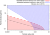 |
Fig. 7 Possible terminal velocities as a function of particle size. The blue hatched area shows velocities towards the negative orbital direction that would enable a particle of given size to remain in the FOV of FORS2 in August 2017. The red area indicates velocities consistent with the observed upper limit of the gas production rate according to Eq. (A5) in Jewitt et al. (2014) and for the parameters described in the text. The overlap region corresponds to combinations of size and backward ejection velocity for particles that could be expected in our image. The solid line represents the velocity-size relationship from Moreno et al. (2013) given in Eq. (6) assuming a bulk density of 1500 kg m−3 and v0 = 25 m s−1. |
4 Summary and discussion
We observed the active asteroid 358P at true anomaly angles of 290.8° and 295.7° and obtain the following key results:
-
The peak-to-peak amplitude of the rotational light curve in August 2017 was likely ~0.2 mag, but might be smaller than that.
-
The 10 h VLT/FORS2 light curve observation does not show an obvious periodicity but might marginally indicate a rotation period of ~8 h.
-
The radial profile of 358P in August 2017 was consistent with that of a point source, showing no evidence of broadening by dust.
-
We derive an average absolute magnitude HR = 19.68 ± 0.01 assuming a C-type phase function, and HR = 19.74 ± 0.01 for an S-type phase function.
-
Assuming a geometric albedo of 0.06, this corresponds to a cross section equivalent sphere of 530 m diameter that has an uncertainty of a factor 1.7 owing to the unknown albedo.
-
For a density of 1500 kg m−3, the surface escape velocity is 0.2 m s−1.
-
Our observation was sensitive to individual fragments >70 m in diameter, which we did not detect.
-
We did not detect a debris trail along the projected orbit, and derive an upper limit to its surface brightness in Cousins R-band of 28.4 mag arcsec−2, three magnitudes fainter than for active asteroids with known debris trails.
-
Our observation is sensitive to dust particles in the size range 8 mm–5 cm, for which we derive an upper limit of 52 × 106 kg produced during the 2012 perihelion passage.
-
The contribution of such particles to the coma brightness in 2012 must have been <10%, while they may still have carried a significant percentage of the ejected mass.
Our primary goal was to study the rotation state of 358P and its possible inter-relation with the activity. We approached this question both directly by measuring the rotational light curve, and indirectly through the size and velocities of the ejected dust.
The latter approach did not yield any indication that fast rotation would be needed to explain the ejection of refractory material. We do not detect large fragments or debris >8 mm, and the derived upper limits are consistent with acceleration by gas drag only.
The direct measurement of the rotational light curve was limited by the unexpected faintness of 358P and the likely small amplitude of the light curve. Our attempt at deriving the rotation period of the target was inconclusive. While a rotation period of ~ 8 h seems compatible with some of our data, it is incompatible with other parts obtained at unfavourable seeing. Our ability to derive a conclusive rotational period might be hampered by the fact that the actual light curve amplitude of the target issmaller than the variability that we measured. This possible explanation is underlined by the fact that our photometric uncertainties are of the same order of magnitude. A different possible explanation for our failing to derive the rotational period might be that the rotation is insufficiently sampled. The period might be much longerthan the 10 h interval for which we observed 358P, or it might be small compared to our cadence (~ 10 min). The latter seems unlikely because it would imply that 358P rotates faster than the critical 2.2 h period applicable for rubble piles, although its size indicates a high probability that 358P is a rubble pile (Warner et al. 2009).
We find some indication of a discrepancy between the average absolute brightness of 358P during our SOAR/Goodman and VLT/FORS2 observations (Sect. 2). A significant variability in brightness is also seen in additional photometry obtained with Gemini South (Mommert et al. 2017), where the corresponding absolute magnitudes fluctuate of the order of 1 mag over the course of several weeks. This might support the idea that the light curve period is longer than the duration of our observation (10 h) or that 358P deviates from a simple periodicity owing to presently unknown reasons. Possible factors adding complexity to the light curve could be the existence of a binary partner, or non-principal axis rotation (“tumbling”). We conclude that we cannot rule out a rotation faster than 10 h if the light curve amplitude (peak-to-peak) is less than ~ 0.2 mag, nor a slow rotation with a period longer than 10 h.
Acknowledgements
J.A. was supported in part by the European Research Council (ERC) Starting Grant No. 757390. M.M. was supported in part by NASA grant No. NNX17AG88G from the Near Earth Object Observations programme. This work is based in part on observationsobtained at the Southern Astrophysical Research (SOAR) telescope, which is a joint project of the Ministério da Ciência, Tecnologia, Inovaçãos e Comunicaçãoes (MCTIC) do Brasil, the U.S. National Optical Astronomy Observatory (NOAO), the University of North Carolina at Chapel Hill (UNC), and Michigan State University (MSU). The results presented in this work are based in part on observations made with ESO Telescopes at the La Silla Paranal Observatory under programme ID 099.C-0530(A). We thank the night astronomer Jesus M. Corral-Santana and the VLT staff for their outstanding work in carrying out the FORS2 observations. We thank the referee for the comments that significantly helped to improve the manuscript. This research has made use of NASA’s Astrophysics Data System Bibliographic Services.
References
- Agarwal, J., Müller, M., Reach, W. T., et al. 2010, Icarus, 207, 992 [NASA ADS] [CrossRef] [Google Scholar]
- Agarwal, J., Jewitt, D., Weaver, H., Mutchler, M., & Larson, S. 2016, AJ, 151, 12 [NASA ADS] [CrossRef] [Google Scholar]
- Agarwal, J., Jewitt, D., Mutchler, M., Weaver, H., & Larson, S. 2017, Nature, 549, 357 [NASA ADS] [CrossRef] [Google Scholar]
- A’Hearn, M. F., Millis, R. L., Schleicher, D. G., Osip, D. J., & Birch, P. V. 1995, Icarus, 118, 223 [NASA ADS] [CrossRef] [Google Scholar]
- Appenzeller, I., Fricke, K., Fürtig, W., et al. 1998, Messenger, 94, 1 [Google Scholar]
- Astropy Collaboration, Robitaille, T. P., Tollerud, E. J., et al. 2013, A&A, 558, A33 [NASA ADS] [CrossRef] [EDP Sciences] [Google Scholar]
- Binney, J., & Merrifield, M. 1998, Galactic Astronomy (Princeton: Princeton University Press) [Google Scholar]
- Bowell, E., Hapke, B., Domingue, D., et al. 1989, in Asteroids II, eds. R. P. Binzel, T. Gehrels, & M. S. Matthews, 524 [Google Scholar]
- Burns, J. A., Lamy, P. L., & Soter, S. 1979, Icarus, 40, 1 [NASA ADS] [CrossRef] [Google Scholar]
- Capria, M. T., Marchi, S., de Sanctis, M. C., Coradini, A., & Ammannito, E. 2012, A&A, 537, A71 [NASA ADS] [CrossRef] [EDP Sciences] [Google Scholar]
- Chambers, K. C., Magnier, E. A., Metcalfe, N., et al. 2016, ArXiv e-prints [arXiv:1612.05560] [Google Scholar]
- Clemens, J. C., Crain, J. A., & Anderson, R. 2004, Proc. SPIE, 5492, 331 [Google Scholar]
- Drahus, M., Waniak, W., Tendulkar, S., et al. 2015, ApJ, 802, L8 [NASA ADS] [CrossRef] [Google Scholar]
- Fanale, F. P., & Salvail, J. R. 1984, Icarus, 60, 476 [NASA ADS] [CrossRef] [Google Scholar]
- Flewelling, H. A., Magnier, E. A., Chambers, K. C., et al. 2016, ArXiv e-prints [arXiv:1612.05243] [Google Scholar]
- Freudling, W., Romaniello, M., Bramich, D. M., et al. 2013, A&A, 559, A96 [NASA ADS] [CrossRef] [EDP Sciences] [Google Scholar]
- Fujiwara, A., Kawaguchi, J., Yeomans, D. K., et al. 2006, Science, 312, 1330 [NASA ADS] [CrossRef] [PubMed] [Google Scholar]
- Giorgini, J. D., Yeomans, D. K., Chamberlin, A. B., et al. 1996, Bull. Am. Astron. Soc., 28, 1158 [Google Scholar]
- Haghighipour, N., Maindl, T. I., Schäfer, C., Speith, R., & Dvorak, R. 2016, ApJ, 830, 22 [NASA ADS] [CrossRef] [Google Scholar]
- Haghighipour, N., Maindl, T. I., Schaefer, C. M., & Wandel, O. J. 2018, ApJ, 855, 60 [NASA ADS] [CrossRef] [Google Scholar]
- Hanuš, J., Viikinkoski, M., Marchis, F., et al. 2017, A&A, 601, A114 [NASA ADS] [CrossRef] [EDP Sciences] [Google Scholar]
- Harris, A. W.,& Lagerros, J. S. V. 2002, Asteroids in the Thermal Infrared, eds. W. F. Bottke, Jr., A. Cellino, P. Paolicchi, & R. P. Binzel, 205 [Google Scholar]
- Hirabayashi, M., & Scheeres, D. J. 2014, ApJ, 780, 160 [NASA ADS] [CrossRef] [Google Scholar]
- Hirabayashi, M., Scheeres, D. J., Sánchez, D. P., & Gabriel, T. 2014, ApJ, 789, L12 [NASA ADS] [CrossRef] [Google Scholar]
- Hsieh, H. H., & Jewitt, D. 2006, Science, 312, 561 [NASA ADS] [CrossRef] [PubMed] [Google Scholar]
- Hsieh, H. H., & Sheppard, S. S. 2015, MNRAS, 454, L81 [NASA ADS] [CrossRef] [Google Scholar]
- Hsieh, H. H., Jewitt, D. C., & Fernández Y. R. 2004, AJ, 127, 2997 [NASA ADS] [CrossRef] [Google Scholar]
- Hsieh, H. H., Meech, K. J., & Pittichová, J. 2011, ApJ, 736, L18 [NASA ADS] [CrossRef] [Google Scholar]
- Hsieh, H. H., Kaluna, H. M., Novaković, B., et al. 2013, ApJ, 771, L1 [NASA ADS] [CrossRef] [Google Scholar]
- Hsieh, H. H., Hainaut, O., Novaković, B., et al. 2015, ApJ, 800, L16 [NASA ADS] [CrossRef] [Google Scholar]
- Ishiguro, M., Hanayama, H., Hasegawa, S., et al. 2011a, ApJ, 740, L11 [NASA ADS] [CrossRef] [Google Scholar]
- Ishiguro, M., Hanayama, H., Hasegawa, S., et al. 2011b, ApJ, 741, L24 [NASA ADS] [CrossRef] [Google Scholar]
- Jewitt, D. 2012, AJ, 143, 66 [NASA ADS] [CrossRef] [Google Scholar]
- Jewitt, D., Agarwal, J., Weaver, H., Mutchler, M., & Larson, S. 2013a, ApJ, 778, L21 [NASA ADS] [CrossRef] [Google Scholar]
- Jewitt, D., Ishiguro, M., & Agarwal, J. 2013b, ApJ, 764, L5 [NASA ADS] [CrossRef] [Google Scholar]
- Jewitt, D., Ishiguro, M., Weaver, H., et al. 2014, AJ, 147, 117 [NASA ADS] [CrossRef] [Google Scholar]
- Jewitt, D., Agarwal, J., Peixinho, N., et al. 2015a, AJ, 149, 81 [NASA ADS] [CrossRef] [Google Scholar]
- Jewitt, D., Hsieh, H., & Agarwal, J. 2015b, in Asteroids IV, eds. P. Michel, F. E. DeMeo, & W. F. Bottke, 221 [Google Scholar]
- Kim, Y., Ishiguro, M., Michikami, T., & Nakamura, A. M. 2017, AJ, 153, 228 [NASA ADS] [CrossRef] [Google Scholar]
- Kresák, L. 1972, Bull. Astr. Inst. Czechosl., 23, 1 [NASA ADS] [Google Scholar]
- Müller, M., Green, S. F., & McBride, N. 2001, in ESA SP-495: Meteoroids 2001 Conference, 47 [Google Scholar]
- Makovoz, D., & Marleau, F. R. 2005, PASP, 117, 1113 [NASA ADS] [CrossRef] [Google Scholar]
- Mommert, M. 2017, Astron. Comput., 18, 47 [NASA ADS] [CrossRef] [Google Scholar]
- Mommert, M., Agarwal, J., Hsieh, H. H., et al. 2017, Cent. Bur. Electronic Tel., 4425, 1 [Google Scholar]
- Moreno, F., Cabrera-Lavers, A., Vaduvescu, O., Licandro, J., & Pozuelos, F. 2013, ApJ, 770, L30 [NASA ADS] [CrossRef] [Google Scholar]
- Nugent, C. R., Mainzer, A., Bauer, J., et al. 2016, AJ, 152, 63 [NASA ADS] [CrossRef] [Google Scholar]
- O’Rourke, L., Snodgrass, C., de Val-Borro, M., et al. 2013, ApJ, 774, L13 [NASA ADS] [CrossRef] [Google Scholar]
- Prialnik, D., & Rosenberg, E. D. 2009, MNRAS, 399, L79 [NASA ADS] [CrossRef] [Google Scholar]
- Schorghofer, N. 2008, ApJ, 682, 697 [NASA ADS] [CrossRef] [Google Scholar]
- Snodgrass, C., Yang, B., & Fitzsimmons, A. 2017, A&A, 605, A56 [NASA ADS] [CrossRef] [EDP Sciences] [Google Scholar]
- Tonry, J. L., Stubbs, C. W., Lykke, K. R., et al. 2012, ApJ, 750, 99 [NASA ADS] [CrossRef] [Google Scholar]
- Wainscoat, R., Hsieh, H., Denneau, L., et al. 2012, Cent. Bur. Electronic Tel., 3252, 1 [NASA ADS] [Google Scholar]
- Warner, B. D., Harris, A. W., & Pravec, P. 2009, Icarus, 202, 134 [NASA ADS] [CrossRef] [Google Scholar]
- Whipple, F. L. 1950, ApJ, 111, 375 [NASA ADS] [CrossRef] [Google Scholar]
All Tables
All Figures
|
Fig. 1 Light curve of 358P on 28 July 2017 observed with SOAR/Goodman (top panel) and on 18 August 2017 observed with VLT/FORS2 (bottom panel). The flux was measured in apertures of radius 1.3D, and for the VLT data set corrected by an offset of –0.09 mag to account for the loss of flux due to the small aperture. This correction was not applied for the SOARdata set because the FWHM was measured as average over the moderately trailed stars. The loss of flux due to the small aperture was therefore less than in the FORS data. The correction would have been small compared to the large scatter and error bars of the data. Open symbols in the bottom panel indicate data obtained after UT 8:00 for comparison with Fig. 2. The scale on the right-hand side vertical axes indicates the derived absolute magnitude according to Eq. (1) and for G = 0.15. The shaded areas in both panels indicate the range of absolute magnitudes covered by the VLT data. |
| In the text | |
|
Fig. 2 Measured magnitude from VLT data as a function of the seeing FWHM, which is proportional to the aperture radius. The two quantities show a weak degree of statistical dependence (R = 0.17). Open symbols indicate data points obtained after UT 8:00 (see Fig. 1.) |
| In the text | |
|
Fig. 3 Spectral power distributions for the light curve period (which corresponds to half the rotation period for a shape-induced double-peaked light curve) of 358P using a statistical approach. For any period in the range, the distributions provide the spectral power as derived with a Lomb–Scargle algorithm; the coloured lines denote different Fourier orders. We are unable to identify a clear periodicity in the period range that was probed. |
| In the text | |
|
Fig. 4 Normalised radial profiles of 358P and field stars in the FORS2 data, measured for two different values of the seeing FWHM, D. The green lines indicate the aperture radius in which the light curve (Fig. 1) was measured and the corresponding flux level of 92%. The x-axis is in units of the FWHM at observation, i.e. a unit interval corresponds to 3.4 pixels for the blue dots and 5.4 pixels for the red dots. |
| In the text | |
|
Fig. 5 358P in a composite of 77 FORS2 exposures, averaged in the co-moving frame of the asteroid. The brightness scale is inverted and linear, and the arrows indicate the anti-solar direction and the projected negative orbital velocity vector. No indication of a debris trail (which should be parallel to the negative velocity vector) is visible. |
| In the text | |
|
Fig. 6 Zoom-in on Fig. 5. The brightness scale is inverted and logarithmic, and the size of the image is 35′′ × 21′′. |
| In the text | |
|
Fig. 7 Possible terminal velocities as a function of particle size. The blue hatched area shows velocities towards the negative orbital direction that would enable a particle of given size to remain in the FOV of FORS2 in August 2017. The red area indicates velocities consistent with the observed upper limit of the gas production rate according to Eq. (A5) in Jewitt et al. (2014) and for the parameters described in the text. The overlap region corresponds to combinations of size and backward ejection velocity for particles that could be expected in our image. The solid line represents the velocity-size relationship from Moreno et al. (2013) given in Eq. (6) assuming a bulk density of 1500 kg m−3 and v0 = 25 m s−1. |
| In the text | |
Current usage metrics show cumulative count of Article Views (full-text article views including HTML views, PDF and ePub downloads, according to the available data) and Abstracts Views on Vision4Press platform.
Data correspond to usage on the plateform after 2015. The current usage metrics is available 48-96 hours after online publication and is updated daily on week days.
Initial download of the metrics may take a while.