| Issue |
A&A
Volume 616, August 2018
|
|
|---|---|---|
| Article Number | A125 | |
| Number of page(s) | 12 | |
| Section | The Sun | |
| DOI | https://doi.org/10.1051/0004-6361/201732251 | |
| Published online | 29 August 2018 | |
Contribution of phase-mixing of Alfvén waves to coronal heating in multi-harmonic loop oscillations
1
School of Mathematics and Statistics, University of St Andrews, North Haugh, St Andrews, Fife, KY16 9SS, UK
e-mail: This email address is being protected from spambots. You need JavaScript enabled to view it.
2
Centre for Fusion, Space and Astrophysics, Department of Physics, University of Warwick, CV4 7AL Coventry, UK
3
Centre for Mathematical Plasma Astrophysics, Mathematics Department, KU Leuven, Celestijnenlaan 200B bus 2400, 3001 Leuven, Belgium
e-mail: This email address is being protected from spambots. You need JavaScript enabled to view it.
Received:
7
November
2017
Accepted:
26
April
2018
Abstract
Context. Kink oscillations of a coronal loop are observed and studied in detail because they provide a unique probe into the structure of coronal loops through magnetohydrodynamics (MHD) seismology and a potential test of coronal heating through the phase mixing of Alfvén waves. In particular, recent observations show that standing oscillations of loops often involve higher harmonics in addition to the fundamental mode. The damping of these kink oscillations is explained by mode coupling with Alfvén waves.
Aims. We investigate the consequences for wave-based coronal heating of higher harmonics and which coronal heating observational signatures we may use to infer the presence of higher harmonic kink oscillations.
Methods. We performed a set of non-ideal MHD simulations in which we modelled the damping of the kink oscillation of a flux tube via mode coupling. We based our MHD simulation parameters on the seismological inversion of an observation for which the first three harmonics are detected. We studied the phase mixing of Alfvén waves, which leads to the deposition of heat in the system, and we applied seismological inversion techniques to the MHD simulation output.
Results. We find that the heating due to phase mixing of Alfvén waves triggered by the damping of kink oscillation is relatively small. We can however illustrate how the heating location drifts from subsequent damping of lower order harmonics. We also address the role of higher order harmonics and the width of the boundary shell in the energy deposition.
Conclusions. We conclude that the coronal heating due to phase mixing does not seem to provide enough energy to maintain the thermal structure of the solar corona even when multi-harmonic oscillations are included; these oscillations play an inhibiting role in the development of smaller scale structures.
Key words: Sun: corona / Sun: helioseismology / Sun: oscillations / Sun: magnetic fields / magnetohydrodynamics (MHD) / waves
© ESO 2018
1. Introduction
The solar corona is a highly dynamic and complex environment where magnetic fields play a key role in shaping coronal structures. Specifically, magnetic loops are ubiquitous in the solar corona and are present in varying lengths and sizes, even if their internal structure remains elusive. Reale (2010) provided a review on the nature of these structures. At the same time, magnetic loops represent a unique laboratory to test coronal heating models owing to their relatively simple structure. To this end coronal seismology is a great support for these investigations as it provides essential information about the properties and geometry of these structures. De Moortel & Browning (2015) and Parnell & De Moortel (2012) provided overviews of the coronal heating problem and the open questions that still need to be addressed.
Many models of coronal heating have relied on the conversion of Alfvén wave energy into thermal energy (see review by Arregui 2015), and in particular the roles of phase mixing of Alfvén waves (Heyvaerts & Priest 1983) and resonant absorption (Goossens et al. 1992, 2002) have been scrutinised.
For these reasons, oscillations of coronal loops have been studied in detail to derive information on the internal structure of the loop and the processes ongoing during the oscillations (Aschwanden et al. 1999, 2002; Aschwanden & Schrijver 2011). Some oscillations are long lived and have minimal damping (e.g. Nisticò et al. 2013; Anfinogentov et al. 2013, 2015; Antolin et al. 2016), while in other circumstances observations clearly show damped oscillations (e.g. Nakariakov et al. 1999; Nisticò et al. 2013; Pascoe et al. 2016b,a). Numerical studies (e.g. Terradas et al. 2008b; Pascoe et al. 2010, 2011) have shown that mode coupling is a viable mechanism to concentrate Alfvén wave energy in thin boundary shells in which small scale structures can form and have suggested that the phase mixing can then convert the wave energy. However, recently Tsiklauri (2016) has claimed that any heating induced by phase mixing is significantly reduced when taking into account plasma flows.
De Moortel & Nakariakov (2012) provided a review of the recent achievement of coronal seismology and Brooks et al. (2012) discussed the structure of coronal loops. In particular, by means of the seismology inversion technique described in Pascoe et al. (2013), which takes into account the Gaussian regime of resonant absorption (Pascoe et al. 2012, 2013; Hood et al. 2013; Ruderman & Terradas 2013), it was possible to derive the properties of the loop and background corona in which the loop oscillation takes place (Pascoe et al. 2016b).
Additionally, there have been indications that the triggering of loop oscillation does not only involve the fundamental kink oscillation mode, but higher parallel harmonics are possibly excited (De Moortel & Brady 2007; Wang et al. 2008; Van Doorsselaere et al. 2007b; Pascoe et al. 2016a). Pascoe et al. (2016b, 2017a) performed detailed analysis of loop oscillations from the catalogue of Zimovets & Nakariakov (2015) and Goddard et al. (2016). The oscillations of the loop were observed with the instrument AIA on board Solar Dynamics Observatory (SDO; Lemen et al. 2012) and were triggered by a nearby eruption. Using Bayesian analysis, Pascoe et al. (2017a) discovered evidence of the second and/or third parallel harmonics being excited for kink oscillations generated by external perturbations (consistent with the numerical simulations by Pascoe et al. 2009 and Pascoe & De Moortel 2014). However, the same analysis found evidence against the existence of higher parallel harmonics for a kink oscillation generated by the postflare implosion (Pascoe et al. 2017c).
These studies have shown that multiple harmonics oscillations are not uncommon in the solar corona and are detectable with current instruments and modelling techniques. Therefore, considering the ongoing investigation on the wave-based heating mechanisms and recent observations of multi-harmonics loop oscillations, we aim to study the effects and observational signatures of additional harmonics on coronal heating.
To carry out our investigation we devise a set of non-ideal magnetohydrodynamic (MHD) simulations in which we model a coronal loop with an inhomogeneous magnetic flux tube whose properties are based on the loop system whose observations are discussed in Pascoe et al. (2017a). Further details on the links between the modelling and observation can be found in Sect. 2. We prescribe a transverse velocity profile along the magnetic flux tube to model the excitation of standing kink oscillations, where the parameters of the initial velocity field are chosen to reproduce the observed multi-harmonic oscillations. The resulting kink oscillations are composed of the first three harmonics of the magnetic flux tube system and they undergo mode coupling by resonant absorption, leading to phase mixing and plasma heating. In order to highlight the role of the higher order harmonics in coronal heating, we consider the heating distribution in time and space correlated with the evolution of each harmonic. From this analysis we derive potential observational signatures of multi-harmonic oscillations related to coronal heating, also comparing different MHD simulations with a different number of harmonics.
The paper is structured as follows. In Sect. 2 we address our MHD modelling and the observation on which particular loop parameters are based. In Sect. 3 we describe the MHD simulations we carry out. In Sect. 4 we carry out a seismology inversion on the output of the MHD simulation and we compare the results with the observations, and we finally discuss results and draw some conclusions in Sect. 5.
2. Model and connection with observation
In order to describe the transverse kink oscillation of a coronal loop and the subsequent mode coupling with Alfvén waves and phase mixing, we devised a model with a magnetised cylinder anchored at each end. The density and Alfvén speed vary across the cylinder and the initial velocity field is used to trigger the transverse kink oscillations. The properties of the flux tube and its oscillation are based on “Loop #1”, which was first analysed seismologically in Pascoe et al. (2016b) and later in Pascoe et al. (2017a); this more recent study extended the method, in particular by considering the presence of parallel harmonics in addition to the fundamental standing mode. Details follow in Sect. 2.1 and Sect. 2.2 for the initial flux tube properties and the initial kink oscillations, respectively.
2.1. Initial condition
We consider a cylindrical flux tube in which we define an interior region, boundary shell, and exterior region (Fig. 1). The system is set in a Cartesian reference frame, where z is the direction along the cylinder axis and x and y define the plane across the cylinder cross section. The origin of the axes is placed at the centre of the cylinder, which corresponds to the loop apex.
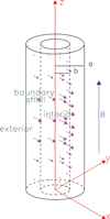 |
Fig. 1. Sketch to illustrate the geometry of our system and the Cartesian axes (red arrows). The blue arrow represents the direction of the magnetic field and the magenta arrows represent the plasma velocity vectors associated with a kink oscillation. The black lines identify the different regions of the loop. |
In the seismological analysis performed on “Loop #1” in Pascoe et al. (2016a), the observations help to constrain the geometrical properties of the loop, such as the loop length, radius, and size of the boundary shell, plasma and magnetic field properties, and density contrast between the interior and exterior regions. The loop length and minor radius were estimated using SDO/AIA 171Å images, which were also used to create time-distance (TD) map showing the loop oscillation. Fitting the position of the loop produced a time series for the loop motion, which allows seismological analysis through the measurement of the period of oscillation and shape of the damping profile. Based on the interpretation in terms of a kink oscillation damped by resonant absorption, these oscillation properties were used to calculate seismological estimates for the loop density contrast ratio and width of the boundary shell. These values are summarised in Table 1, where L is the length of the cylinder, R is the radius of the cylinder, and ∈ is the ratio of the width of the boundary shell to the radius. We relate the radius of the interior region, a, and boundary shell region, b as a = R − 0.5∈R and b = R + 0.5∈R. The value VA is the Alfvén speed in the exterior region, B0 the magnetic field intensity in the same region, and ρc the density contrast ratio of the interior to exterior region. We can derive the density in the exterior region,  , and in the interior, ρi = ρeρc. Finally, we uniformly assign the temperature T0.
In our simulations we modelled the boundary shell using the same density profile as in Pagano & De Moortel (2017)
 (1)
(1)
We note that the density profile in Eq. (1) (depending on tanh) is different from the linear transition layer density profile used in the analysis by Pascoe et al. (2016b), and therefore the definition of the width of the boundary shell. By comparing the two different density profiles we find that the profile above is equivalent to a linear transition layer density profile that is ~10% thinner than the one used in this simulation, for which the damping of kink oscillations by mode coupling is slightly weaker.
The magnetic field is set to have a uniform strength B0 and directed along the z direction, and we set a uniform thermal pressure across the flux tube (2)
(2)
where mp is the proton mass and kb is the Boltzmann constant. These assumptions lead to a magnetohydrostatic configuration in which the temperature varies across the flux tube. Figure 2 shows density and Alfvén speed profile across the centre of the flux tube.
 |
Fig. 2. Profile of density and Alfvén velocity across the cylinder. Dashed lines indicate the borders of the boundary shell a and b. The radius of the cylinder R corresponds to the centre of the boundary shell. |
Parameters obtained from the observations and used for our loop modelling.
2.2. Kink oscillation
To trigger the transverse kink oscillation in the flux tube, we imposed a velocity field in the domain, which corresponds to the linear superposition of the first three standing modes along the extension of the flux tube. The velocity field is uniform within the interior and boundary shell region and the plasma is at rest in the exterior region.
Therefore, in our coordinate system the velocity field inside the interior and boundary shell region only depends on the coordinate z and the three standing modes (n = 1, 2, 3) can be written as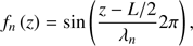 (3)
(3)
where (4)
(4)
In Pascoe et al. (2016a, 2017a) the transverse displacement of Loop #1 is followed at z ≈ 0.4L and in this way it is possible to derive the period of the fundamental mode (the 1st harmonic) and the spatial amplitude of each standing mode. The measured oscillation period of the fundamental mode is P1 = 280 s for the fundamental mode, and consequently the periods for the second (P2 = P1/2) and third mode (P3 = P1/3) can be calculated. The amplitudes for the first three standing modes are estimated as A1 = 1.05 Mm, A2 = 0.35 Mm, and A3 = 0.15 Mm.
In order to model the kink oscillation with an initial velocity field, we transformed these spatial displacement amplitudes into velocity amplitudes by deriving the maximum displacement of the centre of the flux tube from its rest position from the following simple kinematic relation: (5)
(5)
where t is time and Vn is the oscillation velocity amplitude of the nth harmonic. This gives (6)
(6)
However, this simple derivation does not take into account the geometry of the flux tube, the reaction of the plasma surrounding the tube, and the inevitable numerical effects due to the finite resolution. From a test simulation we empirically concluded that we need to multiply Vn, by a factor of 2 to match the modelled displacement at z = 0.4L with the measured value from observation. Table 2 summarises the parameters for the initial velocity field (already multiplied by 2). Figure 3 shows the initial velocity profile along the flux tube that triggers the kink oscillation.
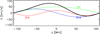 |
Fig. 3. Initial velocity profile along the flux tube (black line) and the contribution from each of the three parallel harmonics: fundamental (green), second (blue), and third (red). |
Parameters oscillation
2.3. MHD numerical set-up
In order to study the evolution of the system after the transverse kink oscillations are initiated, we used the MPI-AMRVAC software (Porth et al. 2014) to solve the MHD equations, where thermal conduction, magnetic diffusion, and joule heating are treated as the following source terms: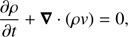 (7)
(7)
 (8)
(8)
 (9)
(9)
 (10)
(10)
where v is the velocity, η the magnetic resistivity, c the speed of light,  the current density, and Fc the conductive flux (Spitzer 1962). The total energy density e is given by
 (11)
(11)
where γ = 5/3 denotes the ratio of specific heats. In our numerical experiments we adopted a value of η that is set uniformly as η = 109ηS , where ηS is the classical value at T = 2 MK (Spitzer 1962).
In order to verify that this value of resistivity leads to appreciable effects above the numerical diffusivity we performed a test simulation with η = 0. We found that a value of η = 109ηS is sufficient to develop significant effects. To better address the evolution of the plasma during the MHD simulation we used tracers to follow the evolution of the plasma that is initially in the interior region (tri), boundary shell (trbs), and exterior region (tre). The tracers tri, trbs, tre can have values between 0 when the tracer is absent and 1 when only the tracer is present and tri + trbs + tre = 1.
The computational domain is composed of 512 × 320 × 256 cells distributed on a uniform grid. The simulation domain extends from x = −8 Mm to x = 8 Mm, from y = −10 Mm to y = 0 Mm (where we model only half of a flux tube), and from z = −110 Mm to z = 110 Mm in the direction of the initial magnetic field. The boundary conditions are implemented using ghost cells, and we set periodic boundary conditions in x, reflective boundary conditions at the y boundary crossing the centre of the flux tube, and outflow boundary conditions at the other y boundary, and fixed boundary conditions at both z boundaries coherently with the oscillation of the standing modes.
3. Results of MHD simulations
In our study we ran a MHD simulation of a transverse kink oscillation of a flux tube where the density and Alfvén speed vary across a boundary shell and the initial kink velocity field is the result of the contribution from the first three harmonics. We focussed our analysis on the generation of Alfvén waves (azimuthal oscillations) in the boundary shell and on the following phase mixing and dissipation of wave energy as heat.
Figure 4 shows maps of density ρ, the x component of the velocity, and the tracers distribution at t = 0, t = P/4, and t = 3P/4 in a projection of the 3D simulation box in which we cut two vertical planes at x = 0 and y = 0 to show the initial oscillation of the flux tube.
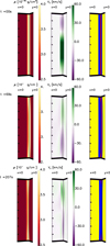 |
Fig. 4. Three-dimensional cuts of the MHD simulation domain showing maps of density ρ (left column), vx (centre column), and the tracers distribution (right column, tri shown in red, trbs shown in blue, and tre shown in yellow) on the x = 0 and y = 0 plane at t = 0 (top row), t = P/4 (middle row), and t = 3P/4 (bottom row). |
We followed the evolution of the system over 5.5 cycles of the fundamental mode, corresponding to approximately 26 min. The oscillation of the flux tube is damped and energy is converted into thermal energy. We verify that energy is conserved within the simulation domain and find that total energy is conserved within 10−3 times its initial value (see Fig. 5).
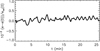 |
Fig. 5. Variation of total energy with time (normalised by its initial value). |
3.1. Evolution of harmonics
The damping of the kink oscillations occurs at different times for different modes owing to the frequency dependence of mode coupling (independent of the damping regime, e.g. the Gaussian or exponential regimes explained in Pascoe et al. 2015). To verify this, we used a minimisation technique to find the best set of parameters to describe the oscillation, both as displacement and as a velocity perturbation.
First, we define the displacement of the flux tube as a function of z and t using the centre of mass of the tracer of the interior region tri as follows: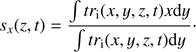 (12)
(12)
At any time t we numerically find the coefficients ws1(t), ws2(t), and ws3(t) that minimise the following function with an accuracy substantially better than the numerical resolution, i.e. (13)
(13)
In other terms we find the best fit for the function sx(z, t) in terms of the three parallel harmonics we initially excited. The same method can be applied to the x component of the velocity perturbation ux
defined as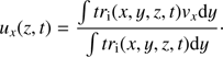 (14)
(14)
To find wu1(t), wu2(t), and wu3(t) we minimise the function χu(t) with an accuracy again substantially better than the numerical accuracy.
Figure 6 shows the evolution of the function χs(t) and χu(t) normalised by the maximum value of the integral of the functions sx(z, t)2 and ux(z, t)2 along the z direction, respectively.
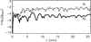 |
Fig. 6. Log of χs(t) (Eq. 13) and χu(t) as a function of time divided by the maximum value of the integral of function sx(z, t)2 and ux(z, t)2 along the z-direction, respectively. |
In Fig. 6 the values of χs(t) and χu(t) remain about three orders of magnitude smaller than the maximum of the functions sx(z, t)2 and ux(z, t)2. This means that the error of representing the oscillation in terms of the first three harmonics is less than 1%. This error is nearly absent at t = 0 when the initial analytic profile can be reconstructed, but it then rises and remains constant. Also, χu(t) remains about an order of magnitude larger than χs(t), as the velocity profile is more complex than the displacement.
Figure 7 shows the evolution of the coefficients ws1(t), ws2(t), and ws3(t) (top panel) and wu1(t), wu2(t), and wu3(t) (bottom panel). Analysing the oscillation either from the point of view of the displacement or velocity perturbation, it is evident that the three parallel harmonics are damped in time and this occurs at different rates. The third harmonic (red line) is the most strongly damped, followed by the second harmonic (blue line), and finally the first harmonic (green line), which remains measurable and is not completely damped by the end of the simulation. The second and third harmonics take between 4 and 5 cycles to be damped. The oscillations in ux are significantly more noisy than those in sx .
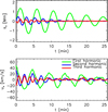 |
Fig. 7. Coefficients for the first three harmonics to fit the displacement of the loop (ws1(t), ws2(t), and ws3(t) – top panel) and the velocity of the loop (wu1(t), wu2(t), and wu3(t) – bottom panel) as a function of time. |
The different damping times of the three harmonics are explained by their different periods. The kink oscillation harmonics are damped as they transfer energy to Alfvén modes in the cylinder boundary and the efficiency of this mode coupling depends linearly on the period of the kink mode (e.g. thin tube approximation by Ruderman & Roberts 2002). If we define the damping time (τn) of the nth harmonic as the time when its maximum oscillation displacement is reduced to about a third of the initial displacement, we find that τ1 = 1480 s, τ2 = 600 s, and τ3 = 355 s. These values depart slightly from a linear dependence, however we note that (i) our flux tube departs from the thin flux tube approximation, (ii) we solve a nonideal MHD equation. and (iii) and our initial kink oscillations is weakly non-linear. Thus our numerical experiment does not entirely satisfy the approximations of analytical approaches such as Ruderman & Roberts (2002).
3.2. Heating
Our model naturally leads to the phase mixing of Alfvén waves generated by mode coupling from the initial kink oscillation of the flux tube. Therefore, the temperature mostly increases where the Alfvén speed has steepest gradients, as larger inhomogeneities favour the phase-mixing rate. In Fig. 8 we show simultaneously the gradient of Alfvén speed and temperature variation from the initial condition in a portion of the x = 0 plane at t = 2P and t = 4P.
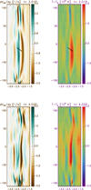 |
Fig. 8. Maps of Alfvén speed gradients (left column) and temperature increase (right column) at t = 2P (top panels) and t = 4P (bottom panels). The arrows in the top panels show where the phase mixing initially develops and leads to a temperature increase. |
We find that at any time there is an evident correlation between the location of steep Alfvén speed gradients and the temperature increase, as the patterns are very similar in the two maps. Additionally, we also find that both Alfvén speed gradient and temperature variation patterns lack symmetry about the z = 0 plane because of the initial asymmetric kink oscillation. The phase mixing quickly develops (top panels) close to z = −20 Mm where the initial peak of the kink velocity is located, as the Alfvén speed gradient is large (either negative or positive) and the temperature increases significantly. At a later stage (bottom panels) the heating is more pronounced near to the centre of the flux tube after the second and third harmonics have been dissipated.
Therefore, we find that the plasma heating connected to the phase mixing of Alfvén waves primarily occurs where the oscillations are stronger and because the Alfvén speed varies only across the boundary shell, we can focus on this specific tracer to investigate this plasma heating process. This approach means that we focussed on the heating due to the actual change of temperature of the plasma and our analysis is not affected by apparent heating such as plasma mixing (due to KHI as in Fig. 11).
In Fig. 9 we plot the average temperature increase for the boundary shell tracer trbs as a function of the coordinate z at different times, where we use different colours for subsequent oscillation cycles.
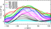 |
Fig. 9. Average temperature increase for the boundary shell tracer trbs as function of z at different times. Different colours denote different oscillation cycles. |
The temperature starts to increase during the first few cycles (light blue and black lines) close to z = −20 Mm, where the initial velocity peak is located. However, in the subsequent cycles we find a higher temperature increase close to z = 0, as the oscillatory motion is dominated by the first harmonic at this stage. Finally, for the last couple of cycles (green and red lines) we see that the temperature increase is saturated close to z = 0 as the lines overlap. At the same time the distribution of temperature increase becomes less peaked and more distributed around the centre. The timescale of this change in the temperature distribution is comparable with the timescale of thermal conduction to thermalise the plasma over approximately 25 Mm.
However, we concluded that the presence of additional harmonics influences the location of the heating as the interference between different harmonics and the different damping times lead to a non-stationary velocity distribution along the flux tube as the velocity peak drifts in time.
A similar behaviour is found on a global scale, i.e. averaging the plasma temperature variation for the boundary shell tracer across the whole domain, as shown in Fig. 10. We see that the temperature remains unaltered for the first 4 min (corresponding to the first cycle) and then it starts to increase roughly linearly in time. After 20 min (approximately 5P), the profile starts to saturate and the temperature increase plateaus at about 40 000 K. This temperature increase corresponds to a very modest deposition of thermal energy in the plasma. A simple estimation of radiative losses (Rosner et al. 1978) over the same time span shows that the energy radiated by the plasma would be about three orders of magnitude larger than the energy deposited by heating.
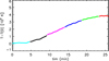 |
Fig. 10. Average temperature increase of the boundary shell tracer as a function of time. The colour table represents different oscillation cycles. |
At the same time, the structure of the flux tube is modified by the development of smaller scale deformations on the boundary layer due to the Kelvin-Helmholtz instabilities (KHI) generated by the azimuthal motions (e.g Terradas et al. 2008a; Antolin et al. 2015; Howson et al. 2017). In Fig. 11 we show the development of these structures at t = 5P on some characteristic cross sections, namely the anti-nodes of the second harmonic (first column) and the anti-nodes of the third harmonic (second column). As expected, the KHI structures lead to a partial fragmentation of the flux tube structure and some mixing of plasma. We also find that the KHI structures do not develop symmetrically about the apex (z = 0) owing to the asymmetric oscillation. As expected, they are more developed on the half of the flux tube where the initial plasma velocity is higher. By comparing the patterns in the cross sections of density and temperature we find that the regions of increased temperature match with those in which the KHI are also more developed, and that the oscillatory motion displaces high temperature regions out of the phase-mixing plane (x = 0).
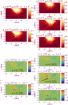 |
Fig. 11. Cross sections of density (top panels) and temperature variation (bottom panels) at t = 5P for different locations. First column: antinodes of the second harmonic. Second column: anti-nodes of the third (and first) harmonic. |
3.3. Fundamental mode simulation
In order to further address how additional parallel harmonics influence the flux tube oscillation dynamics and the following heating we performed a simulation in which only the fundamental mode of the kink oscillation is excited. In this simulation we triggered the initial oscillation with the same kinetic energy that we have initially input in the simulation described in Sect. 3, i.e. 6.7 × 10³ ergs. In this way we aim to determine how the heating deposition is affected by the different harmonics while keeping the initial energy budget unchanged.
Figure 12 summarises this simulation, showing the time dependent evolution of the fundamental mode (as in Fig. 7). We find that the oscillation undergoes more modest damping and that the second and third harmonics are not excited (as expected). In this simulation, the damping of the oscillation is slower than in our reference simulation because the fundamental mode has slower damping times than the higher harmonics whose energy is more quickly transferred to Aflvén modes.
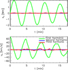 |
Fig. 12. Coefficients for the first three harmonics to fit the displacement of the loop and velocity of the loop as a function of time for the simulation with only the fundamental mode excited by the initial perturbation. |
Moreover, the distribution of the temperature increase is affected by the different velocity profile. Figure 13 shows the temperature increase (for the boundary shell tracer, thus addressing only actual plasma temperature changes) averaged over one period time span for subsequent cycles and compared for the two simulations. We find that the temperature increase peaks at z = 0 in the simulation with only the fundamental mode and it remains symmetric about z = 0. For the first couple of cycles, there seems to be no difference in the total temperature increase, although the heating occurs at different locations. However, from the third cycle the temperature increases more when we excite only the fundamental mode.
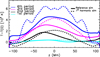 |
Fig. 13. Temperature difference as a function of z averaged over one period. Continuous and dashed lines correspond to simulations with three harmonics or the fundamental mode alone, respectively. |
This is more evident if we plot the averaged temperature increase over the entire numerical domain as function of time (Fig. 14). We find that the temperature increases in a very similar way for the first couple of periods and then the simulation where only the fundamental harmonic is excited shows a temperature increase about 20% larger than the reference simulation.
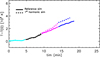 |
Fig. 14. Average temperature increase of the boundary shell tracer as a function of time. The colour table represents different oscillation cycles as in Fig. 9. The continuous line represents the simulation with additional harmonics, while the dashed line represents the simulation with the fundamental mode alone. |
This can be explained by the different initial velocity profiles and how they affect the development of KHI. Figure 15 shows the cross section of density at z = 0 and t = 3.7P for the two simulations. The simulation with only one harmonic shows more developed KHI than that with three harmonics. This also implies that when only the fundamental harmonic is excited, smaller scales develop faster and thus the heating developing from KHI triggers earlier. This can account for the different temperature increase evolution. When only the fundamental harmonic is excited, KHI are generated more efficiently because the damping of this mode by mode coupling is slower than for higher order harmonics and thus higher velocity shears can persist longer. Additionally, the interference between the three harmonics is not always constructive and at times this can reduce the shear velocity between the oscillating flux tube and its surroundings. A coherent fundamental mode oscillation is not affected by that.
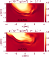 |
Fig. 15. Comparison of the cross sections of the density for the simulations with 3 harmonics (top panel) and with 1 harmonic (bottom panel) at the centre of the flux tube z = 0 at t = 3.7 P, which shows the different development of the KHI in the two simulations. |
3.4. Boundary shell
We also considered the role of the width of the boundary shell in the phase-mixing heating process. We performed an additional simulation with a boundary layer half the size of that used in the simulation presented in Sect. 3.
As discussed in Pagano & De Moortel (2017), the width of the boundary shell plays two competing roles in this set-up. On one hand, the efficiency of the mode coupling from kink oscillations to Alfvén waves is proportional to the width of the boundary shell. On the other hand the efficiency of the phase-mixing mechanism is inversely proportional to the width of the boundary shell. Thus the energy deposition is not significantly affected by the width of the boundary shell, while the temperature increase is slightly affected, as roughly the same amount of energy is deposited in a smaller volume.
This behaviour is also confirmed in this study. In Fig. 16, we plot the temperature variation (for the boundary shell tracer, thus addressing only actual plasma temperature changes) along the flux tube averaged over each cycle. We find that the two simulations behave very similarly and only develop a significant difference after five cycles when the small scales generated by KHI are more diffused.
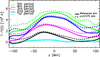 |
Fig. 16. Temperature change with respect to the initial value as a function of z averaged over one period oscillation for subsequent oscillations identified with various colours. Continuous line for simulation with ∈ = 1.15 and dashed line for simulation with ∈ = 0.575. |
By following the temperature increase averaged over the whole domain (Fig. 17) we find that the two simulations show a very similar temperature increase and that the thinner boundary simulation shows only a 2% larger temperature increase. The energy deposited by the mode coupling and then phase mixing is not dependent on the width of the boundary shell. However, a thinner boundary shell leads to higher temperatures since the same thermal energy is deposited in a smaller region.
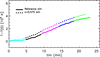 |
Fig. 17. Average temperature change with respect to the initial value of the boundary shell tracer plasma as a function of time. The colour table represents various oscillation cycles as in Fig. 9. The continuous and dashed lines represent simulations with thicker and thinner boundary shells, respectively. |
4. Comparison with observations
In this section, we analyse our simulation data using the seismological techniques from Pascoe et al. (2017b). These techniques are based on the analysis of extreme ultraviolet (EUV) imaging data. We may use our simulation data to generate the forward-modelled EUV intensity for a particular instrument and bandpass such as SDO/AIA 171Å used in the observational analysis. However, for the purpose of this study we use a simpler approximation of calculating the intensity as ρ2T integrated along the line of sight (y coordinate). We create a TD map for z = −22 Mm, which corresponds to the position 0.4L and is comparable to the position of the observational slit used for Loop #1 in Pascoe et al. (2016a). This allows us to generate a TD map that may be used in the same observational analysis routines used for observational data, but preserving the greater spatial resolution provided by our numerical data.
Figures 18 and 19 show the results of estimating the transverse density profile by forward modelling of the EUV intensity profile (Pascoe et al. 2017b; Goddard et al. 2017); we note that the effect of the point spread function is not considered. Figure 18 shows the TD map with the position of the loop shown by the green line corresponding to the maximum a posteriori probability value returned by Markov chain Monte Carlo (MCMC) sampling. Figure 19 shows the variation of R, ∈, A, and the normalised leg mass (per unit length) during the oscillation. We find a gradual increase in ∈ after about a period of oscillation. These results are consistent with (Goddard et al. in prep.) who find the signatures of KHI on a forward modelled loop core to include a widening inhomogeneous layer and an approximately stationary radius. However, in contrast to that study, we find an increasing rather than decreasing intensity associated with the loop heating. Localised KHI structures are also responsible for the rapid changes in ∈ values, whereas our fit is based on a single loop without this fine structuring. We also note that Fig. 18 shows additional waves outside the loop corresponding to propagating fast waves. These can contribute to the variation of density profile parameters with a short periodicity determined by the small size of the numerical domain in the directions transverse to the loop axis. Also Antolin et al. (2017) found that the onset of KHI leads to the apparent broadening of the boundary shell in forward-modelled observations.
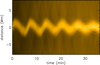 |
Fig. 18. Time-distance map of the quantity ρ2T integrated along the LOS at z = 0.4L. |
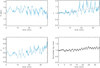 |
Fig. 19. Time-dependence of the transverse density profile parameters R (top left), ∈ (top right), and A (bottom left) estimated by forward modelling of the transverse intensity profile. The symbols indicate the maximum a posteriori probability values and the shaded regions correspond to the 95% credible intervals. The bottom right panel shows the variation in leg mass per unit length. |
There is also a gradual increase of approximately 10% in the leg mass by the end of the simulation and a short period oscillation that begins at the same time as the KHI onset time. This is consistent with KHI generating fine structuring in the inhomogeneous layer, which affects the estimate of the monolithic loop profile used by the forward modelling method and based on the linear transition layer profile.
Figure 20 shows the results of the seismological analysis of the kink oscillation. These panels may be compared with Fig. 6 of Pascoe et al. (2017a) with which there is good agreement. The dashed lines correspond to limiting approximations based on the Gaussian damping profile being dominant for low density contrasts and the exponential damping profile for high density contrasts (Hood et al. 2013; Pascoe et al. 2013). As in the case of the observational data, because the oscillation is well described by a Gaussian damping profile implies a loop with a low density contrast ratio. This provides an estimate of the upper limit of ρ0/ρe ≲ 2, in addition to the lower limit prescribed by the overall damping rate. On the other hand, for the low density contrast regime the inhomogeneous layer width is weakly constrained by the seismological method to ∈ ≳ 0.5 due to the asymptotic behaviour (e.g. Arregui et al. 2007). The estimated density contrasts are slightly lower than the density contrast of ρc = 1.7 used in the MHD initial condition. However, this method is based on the thin boundary approximation, whereas our simulation is for ∈χ 1. The difference of approximately 20% is consistent with the study of the effect of large inhomogeneous layers on the resonant absorption damping time (for the exponential damping regime) performed by Van Doorsselaere et al. (2004).
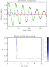 |
Fig. 20. Results of the seismological analysis of the loop oscillation. The top panel shows the detrended loop position (symbols) with the first (green), second (blue), and third (red) parallel harmonics. The bottom panel shows the density profile parameters determined by the oscillation damping envelope. The dashed lines correspond to estimates for the lower limits of the density contrast ratio and inhomogeneous layer width. |
5. Discussion and conclusions
In this work we have carried out MHD simulations to study how the excitation of multiple parallel harmonics of standing kink oscillations in coronal loops influences the heating associated with the phase mixing of Alfvén waves. The work is motivated by the observation of multi-harmonics oscillations in Pascoe et al. (2017a). Our modelling focusses on a magnetised flux tube anchored at its footpoints, where an initial velocity field is set to trigger the oscillation of the first three kink oscillation harmonics. The properties of the flux tube and the initial velocity distribution are based on a particular kink oscillation observed in Pascoe et al. (2017a), namely a loop with a low density contrast ratio, a wide inhomogenous layer, and observed to support three standing kink mode harmonics.
In order to study the heating of the plasma due to the phase mixing of Alfvén waves, we first performed an analysis where we fit the flux tube oscillation with the first three harmonics. We additionally ran a set of MHD simulations, where we varied the number of harmonics initially excited, as well at the width of the boundary shell. Moreover, we also applied a seismology inversion to the MHD data to test the robustness of our model and to highlight what information can be derived from the seismology on the internal structure of coronal loops.
In the present study, we have found that the plasma heating that follows from the phase mixing of Alfvén waves is a marginal portion of the energy budget needed to maintain the thermal structure of coronal loops, as the energy deposited is much smaller than the energy lost by radiation by the plasma, where the model energy input was not arbitrary but constrained by the oscillations observed by Pascoe et al. (2016b, 2017a). Previously Cargill et al. (2016) and Pagano & De Moortel (2017) raised concerns about whether phase mixing could be effective in providing the energy budget to support the coronal thermal structure. At the same time, it is still possible that oscillations are only a component of the process that leads to coronal heating, which is ultimately enhanced by turbulence or reconnection phenomena, as suggested by several modelling studies, such as Reale et al. (2016) and Dahlburg et al. (2016). Therefore, it is still not possible to rule out phase mixing as a heating mechanism without high spatial resolution and high cadence observations providing better estimates of the wave energy that is present in the solar corona (e.g. De Moortel & Pascoe 2012).
Nonetheless, some useful information can be gained from the analysis of the flux tube oscillation dynamics when higher order harmonics are included. We find that the presence of multiple harmonics affects the heating of the flux tube in two ways. Firstly, it affects the location of the heating the deposition. The heating is mostly localised in the position along the flux tube where more kinetic energy is initially available for conversion. This is a consequence of the fact that the phase mixing of Alfvén waves is a process that starts while the mode coupling of the kink oscillation is still ongoing, i.e. the mode coupling and phase mixing are not occurring consecutively, but rather simultaneously. Therefore, depending on the relative amplitude and phase of the harmonics involved, the heating is mostly localised in the position along the flux tube where the kink velocity profile peaks. Moreover, as different harmonics have different damping times in the mode coupling process, the location of the velocity peak changes as higher harmonics disappear. In our study this leads to a drift of the heating location towards the apex of the coronal loop, as the fundamental harmonic has the longest damping time.
Secondly, when the kink oscillation kinetic energy is distributed among multiple harmonics, the heating process is less effective if KHI is also involved in the process. In fact, we found that the coherent motion of one single harmonic leads to the highest velocity difference between the loop structure and the environment, thus allowing the strongest development of KHI in the boundary layer. After the small scale structures are developed, the heating becomes more efficient. In contrast, the interference between several harmonics is not always constructive and this results in lower oscillatory motion and thus slower formation of KHI. A number of studies have already shown that KHI is sensitive to the relative motion between the oscillating structures and the environment (Browning & Priest 1984; Terradas et al. 2008a; Foullon et al. 2011; Antolin et al. 2015; Okamoto et al. 2015; Magyar & Van Doorsselaere 2016; Howson et al. 2017; Karampelas et al. 2017). Our work implies that the presence of higher order harmonics is one of the factors that inhibits or delays the formation of KHI and it should be taken into account when deriving loop properties from the development of small scale structures. Goddard & Nakariakov (2016) also found that smaller amplitude oscillations persist for longer, also suggesting that non-linear effects (such as the development of small scales) accelerate the damping of the oscillation.
Karampelas et al. (2017) and Van Doorsselaere et al. (2007a) argued that heating directly due to resistivity and viscosity can take place at different locations of the flux tube, as the first occurs through the dissipation of electric currents and the second of velocity shears. Our simulation partially confirms this suggestion. In fact, by comparing our simulation with a simulation where we set η = 0 we find that the effect of resistivity is more visible at the footpoints, where currents induced by the oscillation are stronger, than near to the centre of the flux tube, where the current is smaller, but the velocity shear is higher. At the same time, a known effect of mode coupling of Alfvén waves is to eventually concentrate energy into a small region and the main effect of KHI is to further fragment these structures and to generate new currents, while the currents induced by oscillations become weaker because of the damping of the kink modes. Therefore, it is reasonable to assume that in this scenario the heat deposition at the centre of the flux tube eventually prevails on the footpoint heating. This also suggests that our results are due to a combination of the effects of numerical viscosity whose impact increases with high velocity gradients and the effects of magnetic resistivity dissipating the small scale currents developed by phase mixing and KHI.
It should also be noted that the line-tied boundary conditions used in MHD simulations to model the behaviour of loop footpoints probably lead to an overestimation of the electric currents generated at these locations by standing modes, as it has not been thoroughly investigated whether coronal loops are perfectly anchored at their coronal footpoints during kink oscillations.
It is also worth addressing the differences between our model and the observations that inspired our MHD simulation parameters. In our simulation the oscillation of the fundamental mode is still visible after 5P, while it is not the case in the observation that is nearly completely damped after 4P. There are several modelling parameters that can justify this discrepancy that cannot be resolved by the observations, but still affect the exact dynamics of the loop. One is the density profile we have assumed Sect. 2.1. However, seismological techniques developed thus far are also based on the thin boundary approximation, which is not applicable to our simulations specifically, and coronal loops in general (e.g. statistical study by Goddard et al. 2017). The consequence of this approximation is an error of ~ 20% in current seismological inversions. The damping rate in our simulations is also affected by numerical effects due to finite resolution.
Finally, this study also hints that details of the loop internal structure, such as the radius of the internal structure or the width of the boundary shell, may be inferred from seismological and forward modelling techniques (see Fig. 19), which shows changes in the estimates of ∈ and R occur following the development of KHI.
Acknowledgments
This research has received funding from the Science and Technology Facilities Council (UK) through the consolidated grant ST/N000609/1 and the European Research Council (ERC) under the European Union’s Horizon 2020 research and innovation programme (grant agreement No. 647214). This work is supported by the European Research Council under the SeismoSun Research Project No. 321141 (DJP). This project has received funding from the European Research Council (ERC) under the European Union’s Horizon 2020 research and innovation programme (grant agreement No 724326). This work used the DiRAC Data Centric system at Durham University, operated by the Institute for Computational Cosmology on behalf of the STFC DiRAC HPC Facility (www.dirac.ac.uk). This equipment was funded by a BIS National E-infrastructure capital grant ST/K00042X/1, STFC capital grant ST/K00087X/1, DiRAC Operations grant ST/K003267/1 and Durham University. DiRAC is part of the National E-Infrastructure. We acknowledge the use of the open source (gitorious.org/amrvac) MPI-AMRVAC software, relying on coding efforts from C. Xia, O. Porth, R. Keppens.
References
- Anfinogentov, S., Nisticò, G., & Nakariakov, V. M. 2013, A&A, 560, A107 [NASA ADS] [CrossRef] [EDP Sciences] [Google Scholar]
- Anfinogentov, S. A., Nakariakov, V. M., & Nisticò, G. 2015, A&A, 583, A136 [NASA ADS] [CrossRef] [EDP Sciences] [Google Scholar]
- Antolin, P., Okamoto, T. J., De Pontieu, B., et al. 2015, ApJ, 809, 72 [NASA ADS] [CrossRef] [Google Scholar]
- Antolin, P., De Moortel, I., Van Doorsselaere, T., & Yokoyama, T. 2016, ApJ, 830, L22 [Google Scholar]
- Antolin, P., De Moortel, I., Van Doorsselaere, T., & Yokoyama, T. 2017, ApJ, 836, 219 [NASA ADS] [CrossRef] [Google Scholar]
- Arregui, I. 2015, Philos. Trans. R. Soc. London, Ser. A, 373, 20140261 [Google Scholar]
- Arregui, I., Andries, J., Van Doorsselaere, T., Goossens, M., & Poedts, S. 2007, A&A, 463, 333 [NASA ADS] [CrossRef] [EDP Sciences] [Google Scholar]
- Aschwanden, M. J., & Schrijver, C. J. 2011, ApJ, 736, 102 [NASA ADS] [CrossRef] [Google Scholar]
- Aschwanden, M. J., Fletcher, L., Schrijver, C. J., & Alexander, D. 1999, ApJ, 520, 880 [NASA ADS] [CrossRef] [Google Scholar]
- Aschwanden, M. J., de Pontieu, B., Schrijver, C. J., & Title, A. M. 2002, Sol. Phys., 206, 99 [NASA ADS] [CrossRef] [Google Scholar]
- Brooks, D. H., Warren, H. P., & Ugarte-Urra, I. 2012, ApJ, 755, L33 [NASA ADS] [CrossRef] [Google Scholar]
- Browning, P. K., & Priest, E. R. 1984, A&A, 131, 283 [NASA ADS] [Google Scholar]
- Cargill, P. J., De Moortel, I., & Kiddie, G. 2016, ApJ, 823, 31 [NASA ADS] [CrossRef] [Google Scholar]
- Dahlburg, R. B., Einaudi, G., Taylor, B. D., et al. 2016, ApJ, 817, 47 [NASA ADS] [CrossRef] [Google Scholar]
- De Moortel, I., & Brady, C. S. 2007, ApJ, 664, 1210 [NASA ADS] [CrossRef] [Google Scholar]
- De Moortel, I., & Browning, P. 2015, Philos. Trans. R. Soc. London, Ser. A, 373, 20140269 [Google Scholar]
- De Moortel, I., & Nakariakov, V. M. 2012, Philos. Trans. R. Soc. London, Ser. A, 370, 3193 [Google Scholar]
- De Moortel, I., & Pascoe, D. J. 2012, ApJ, 746, 31 [NASA ADS] [CrossRef] [Google Scholar]
- Foullon, C., Verwichte, E., Nakariakov, V. M., Nykyri, K., & Farrugia, C. J. 2011, ApJ, 729, L8 [NASA ADS] [CrossRef] [Google Scholar]
- Goddard, C. R., & Nakariakov, V. M. 2016, A&A, 590, L5 [NASA ADS] [CrossRef] [EDP Sciences] [Google Scholar]
- Goddard, C. R., Nisticò, G., Nakariakov, V. M., & Zimovets, I. V. 2016, A&A, 585, A137 [NASA ADS] [CrossRef] [EDP Sciences] [Google Scholar]
- Goddard, C. R., Pascoe, D. J., Anfinogentov, S., & Nakariakov, V. M. 2017, A&A, 605, A65 [NASA ADS] [CrossRef] [EDP Sciences] [Google Scholar]
- Goossens, M., Hollweg, J. V., & Sakurai, T. 1992, Sol. Phys., 138, 233 [NASA ADS] [CrossRef] [Google Scholar]
- Goossens, M., Andries, J., & Aschwanden, M. J. 2002, A&A, 394, L39 [NASA ADS] [CrossRef] [EDP Sciences] [Google Scholar]
- Heyvaerts, J., & Priest, E. R. 1983, A&A, 117, 220 [NASA ADS] [Google Scholar]
- Hood, A. W., Ruderman, M., Pascoe, D. J., et al. 2013, A&A, 551, A39 [NASA ADS] [CrossRef] [EDP Sciences] [Google Scholar]
- Howson, T. A., De Moortel, I., & Antolin, P. 2017, A&A, 602, A74 [NASA ADS] [CrossRef] [EDP Sciences] [Google Scholar]
- Karampelas, K., Van Doorsselaere, T., & Antolin, P. 2017, A&A, 604, A130 [NASA ADS] [CrossRef] [EDP Sciences] [Google Scholar]
- Lemen, J. R., Title, A. M., Akin, D. J., et al. 2012, Sol. Phys., 275, 17 [NASA ADS] [CrossRef] [Google Scholar]
- Magyar, N., & Van Doorsselaere, T. 2016, A&A, 595, A81 [NASA ADS] [CrossRef] [EDP Sciences] [Google Scholar]
- Nakariakov, V. M., Ofman, L., Deluca, E. E., Roberts, B., & Davila, J. M. 1999, Science, 285, 862 [NASA ADS] [CrossRef] [PubMed] [Google Scholar]
- Nisticò, G., Nakariakov, V. M., & Verwichte, E. 2013, A&A, 552, A57 [NASA ADS] [CrossRef] [EDP Sciences] [Google Scholar]
- Okamoto, T. J., Antolin, P., De Pontieu, B., et al. 2015, ApJ, 809, 71 [NASA ADS] [CrossRef] [Google Scholar]
- Pagano, P., & De Moortel, I. 2017, A&A, 601, A107 [NASA ADS] [CrossRef] [EDP Sciences] [Google Scholar]
- Parnell, C. E., & De Moortel, I. 2012, Philos. Trans. R. Soc. London, Ser. A, 370, 3217 [Google Scholar]
- Pascoe, D. J., & De Moortel, I. 2014, ApJ, 784, 101 [NASA ADS] [CrossRef] [Google Scholar]
- Pascoe, D. J., de Moortel, I., & McLaughlin, J. A. 2009, A&A, 505, 319 [NASA ADS] [CrossRef] [EDP Sciences] [Google Scholar]
- Pascoe, D. J., Wright, A. N., & De Moortel, I. 2010, ApJ, 711, 990 [NASA ADS] [CrossRef] [Google Scholar]
- Pascoe, D. J., Wright, A. N., & De Moortel, I. 2011, ApJ, 731, 73 [NASA ADS] [CrossRef] [Google Scholar]
- Pascoe, D. J., Hood, A. W., de Moortel, I., & Wright, A. N. 2012, A&A, 539, A37 [NASA ADS] [CrossRef] [EDP Sciences] [Google Scholar]
- Pascoe, D. J., Hood, A. W., De Moortel, I., & Wright, A. N. 2013, A&A, 551, A40 [NASA ADS] [CrossRef] [EDP Sciences] [Google Scholar]
- Pascoe, D. J., Wright, A. N., De Moortel, I., & Hood, A. W. 2015, A&A, 578, A99 [NASA ADS] [CrossRef] [EDP Sciences] [Google Scholar]
- Pascoe, D. J., Goddard, C. R., & Nakariakov, V. M. 2016a, A&A, 593, A53 [NASA ADS] [CrossRef] [EDP Sciences] [Google Scholar]
- Pascoe, D. J., Goddard, C. R., Nisticò, G., Anfinogentov, S., & Nakariakov, V. M. 2016b, A&A, 589, A136 [NASA ADS] [CrossRef] [EDP Sciences] [Google Scholar]
- Pascoe, D. J., Anfinogentov, S., Nisticò, G., Goddard, C. R., & Nakariakov, V. M. 2017a, A&A, 600, A78 [NASA ADS] [CrossRef] [EDP Sciences] [Google Scholar]
- Pascoe, D. J., Goddard, C. R., Anfinogentov, S., & Nakariakov, V. M. 2017b, A&A, 600, L7 [NASA ADS] [CrossRef] [EDP Sciences] [Google Scholar]
- Pascoe, D. J., Russell, A. J. B., Anfinogentov, S. A., et al. 2017c, A&A, 607, A8 [NASA ADS] [CrossRef] [EDP Sciences] [Google Scholar]
- Porth, O., Xia, C., Hendrix, T., Moschou, S. P., & Keppens, R. 2014, ApJS, 214, 4 [Google Scholar]
- Reale, F. 2010, Liv. Rev. Sol. Phys., 7, 5 [Google Scholar]
- Reale, F., Orlando, S., Guarrasi, M., et al. 2016, ApJ, 830, 21 [NASA ADS] [CrossRef] [Google Scholar]
- Rosner, R., Tucker, W. H., & Vaiana, G. S. 1978, ApJ, 220, 643 [NASA ADS] [CrossRef] [Google Scholar]
- Ruderman, M. S., & Roberts, B. 2002, ApJ, 577, 475 [NASA ADS] [CrossRef] [Google Scholar]
- Ruderman, M. S., & Terradas, J. 2013, A&A, 555, A27 [NASA ADS] [CrossRef] [EDP Sciences] [Google Scholar]
- Spitzer, L. 1962, in Physics of Fully Ionized Gases, 2nd edition (New York: Interscience) [Google Scholar]
- Terradas, J., Andries, J., Goossens, M., et al. 2008a, ApJ, 687, L115 [Google Scholar]
- Terradas, J., Arregui, I., Oliver, R., et al. 2008b, ApJ, 679, 1611 [NASA ADS] [CrossRef] [Google Scholar]
- Tsiklauri, D. 2016, A&A, 586, A95 [NASA ADS] [CrossRef] [EDP Sciences] [Google Scholar]
- Van Doorsselaere, T., Andries, J., Poedts, S., & Goossens, M. 2004, ApJ, 606, 1223 [NASA ADS] [CrossRef] [Google Scholar]
- Van Doorsselaere, T., Andries, J., & Poedts, S. 2007a, A&A, 471, 311 [NASA ADS] [CrossRef] [EDP Sciences] [Google Scholar]
- Van Doorsselaere, T., Nakariakov, V. M., & Verwichte, E. 2007b, A&A, 473, 959 [NASA ADS] [CrossRef] [EDP Sciences] [Google Scholar]
- Wang, T. J., Solanki, S. K., & Selwa, M. 2008, A&A, 489, 1307 [NASA ADS] [CrossRef] [EDP Sciences] [Google Scholar]
- Zimovets, I. V., & Nakariakov, V. M. 2015, A&A, 577, A4 [NASA ADS] [CrossRef] [EDP Sciences] [Google Scholar]
All Tables
All Figures
|
Fig. 1. Sketch to illustrate the geometry of our system and the Cartesian axes (red arrows). The blue arrow represents the direction of the magnetic field and the magenta arrows represent the plasma velocity vectors associated with a kink oscillation. The black lines identify the different regions of the loop. |
| In the text | |
|
Fig. 2. Profile of density and Alfvén velocity across the cylinder. Dashed lines indicate the borders of the boundary shell a and b. The radius of the cylinder R corresponds to the centre of the boundary shell. |
| In the text | |
|
Fig. 3. Initial velocity profile along the flux tube (black line) and the contribution from each of the three parallel harmonics: fundamental (green), second (blue), and third (red). |
| In the text | |
|
Fig. 4. Three-dimensional cuts of the MHD simulation domain showing maps of density ρ (left column), vx (centre column), and the tracers distribution (right column, tri shown in red, trbs shown in blue, and tre shown in yellow) on the x = 0 and y = 0 plane at t = 0 (top row), t = P/4 (middle row), and t = 3P/4 (bottom row). |
| In the text | |
|
Fig. 5. Variation of total energy with time (normalised by its initial value). |
| In the text | |
|
Fig. 6. Log of χs(t) (Eq. 13) and χu(t) as a function of time divided by the maximum value of the integral of function sx(z, t)2 and ux(z, t)2 along the z-direction, respectively. |
| In the text | |
|
Fig. 7. Coefficients for the first three harmonics to fit the displacement of the loop (ws1(t), ws2(t), and ws3(t) – top panel) and the velocity of the loop (wu1(t), wu2(t), and wu3(t) – bottom panel) as a function of time. |
| In the text | |
|
Fig. 8. Maps of Alfvén speed gradients (left column) and temperature increase (right column) at t = 2P (top panels) and t = 4P (bottom panels). The arrows in the top panels show where the phase mixing initially develops and leads to a temperature increase. |
| In the text | |
|
Fig. 9. Average temperature increase for the boundary shell tracer trbs as function of z at different times. Different colours denote different oscillation cycles. |
| In the text | |
|
Fig. 10. Average temperature increase of the boundary shell tracer as a function of time. The colour table represents different oscillation cycles. |
| In the text | |
|
Fig. 11. Cross sections of density (top panels) and temperature variation (bottom panels) at t = 5P for different locations. First column: antinodes of the second harmonic. Second column: anti-nodes of the third (and first) harmonic. |
| In the text | |
|
Fig. 12. Coefficients for the first three harmonics to fit the displacement of the loop and velocity of the loop as a function of time for the simulation with only the fundamental mode excited by the initial perturbation. |
| In the text | |
|
Fig. 13. Temperature difference as a function of z averaged over one period. Continuous and dashed lines correspond to simulations with three harmonics or the fundamental mode alone, respectively. |
| In the text | |
|
Fig. 14. Average temperature increase of the boundary shell tracer as a function of time. The colour table represents different oscillation cycles as in Fig. 9. The continuous line represents the simulation with additional harmonics, while the dashed line represents the simulation with the fundamental mode alone. |
| In the text | |
|
Fig. 15. Comparison of the cross sections of the density for the simulations with 3 harmonics (top panel) and with 1 harmonic (bottom panel) at the centre of the flux tube z = 0 at t = 3.7 P, which shows the different development of the KHI in the two simulations. |
| In the text | |
|
Fig. 16. Temperature change with respect to the initial value as a function of z averaged over one period oscillation for subsequent oscillations identified with various colours. Continuous line for simulation with ∈ = 1.15 and dashed line for simulation with ∈ = 0.575. |
| In the text | |
|
Fig. 17. Average temperature change with respect to the initial value of the boundary shell tracer plasma as a function of time. The colour table represents various oscillation cycles as in Fig. 9. The continuous and dashed lines represent simulations with thicker and thinner boundary shells, respectively. |
| In the text | |
|
Fig. 18. Time-distance map of the quantity ρ2T integrated along the LOS at z = 0.4L. |
| In the text | |
|
Fig. 19. Time-dependence of the transverse density profile parameters R (top left), ∈ (top right), and A (bottom left) estimated by forward modelling of the transverse intensity profile. The symbols indicate the maximum a posteriori probability values and the shaded regions correspond to the 95% credible intervals. The bottom right panel shows the variation in leg mass per unit length. |
| In the text | |
|
Fig. 20. Results of the seismological analysis of the loop oscillation. The top panel shows the detrended loop position (symbols) with the first (green), second (blue), and third (red) parallel harmonics. The bottom panel shows the density profile parameters determined by the oscillation damping envelope. The dashed lines correspond to estimates for the lower limits of the density contrast ratio and inhomogeneous layer width. |
| In the text | |
Current usage metrics show cumulative count of Article Views (full-text article views including HTML views, PDF and ePub downloads, according to the available data) and Abstracts Views on Vision4Press platform.
Data correspond to usage on the plateform after 2015. The current usage metrics is available 48-96 hours after online publication and is updated daily on week days.
Initial download of the metrics may take a while.