| Issue |
A&A
Volume 616, August 2018
|
|
|---|---|---|
| Article Number | A99 | |
| Number of page(s) | 8 | |
| Section | The Sun | |
| DOI | https://doi.org/10.1051/0004-6361/201730990 | |
| Published online | 27 August 2018 | |
Rotating network jets in the quiet Sun as observed by IRIS
1
Group of Astrophysics, University of Maria Curie-Skłodowska,
ul. Radziszewskiego 10,
20-031
Lublin, Poland
2
Department of Physics, Indian Institute of Technology (Banaras Hindu University),
Varanasi
22105, India
Received:
16
April
2017
Accepted:
3
May
2018
Abstract
Aims. We perform a detailed observational analysis of network jets to understand their kinematics, rotational motion, and underlying triggering mechanism(s). We analyzed the quiet-Sun (QS) data.
Methods. IRIS high-resolution imaging and spectral observations (slit-jaw images: Si IV 1400.0 Å; raster: Si IV 1393.75 Å) were used to analyze the omnipresent rotating network jets in the transition region (TR). In addition, we also used observations from the Atmospheric Imaging Assembly (AIA) on board the Solar Dynamic Observation (SDO).
Results. The statistical analysis of 51 network jets is performed to understand their various mean properties, e.g., apparent speed (140.16 ± 39.41 km s−1), length (3.16 ± 1.18 Mm), and lifetimes (105.49 ± 51.75 s). The Si IV 1393.75 Å line has a secondary component along with its main Gaussian, which is formed due to the high-speed plasma flows (i.e., network jets). The variation in Doppler velocity across these jets (i.e., blueshift on one edge and redshift on the other) signify the presence of inherited rotational motion. The statistical analysis predicts that the mean rotational velocity (i.e., ΔV) is 49.56 km s−1. The network jets have high-angular velocity in comparison to the other class of solar jets.
Conclusions. The signature of network jets is inherited in TR spectral lines in terms of the secondary component of the Si IV 1393.75 Å line. The rotational motion of network jets is omnipresent, which is reported first for this class of jet-like features. The magnetic reconnection seems to be the most favorable mechanism for the formation of these network jets.
Key words: Sun: activity / Sun: corona / Sun: transition region / magnetohydrodynamics (MHD) / methods: numerical
© ESO 2018
1 Introduction
Various kinds of jet-like structures (spicules, chromospheric anemone jets, macrospicules, surges, X-ray/UV/EUV jets, etc.) are episodically present in the solar atmosphere. The study of these jet-like structures is one of the important areas in solar physics research using observations/numerical simulations. Therefore, our depth of knowledge about them and their formation, evolution, plasma properties, etc., is continuously improving (e.g., Bohlin et al. 1975; Schmieder et al. 1995; Yokoyama & Shibata 1995; Canfield et al. 1996; Yokoyama & Shibata 1996; Chae et al. 1999; Wilhelm 2000; De Pontieu et al. 2004, 2007; Cirtain et al. 2007; Shibata et al. 2007; Nishizuka et al. 2008; Murawski & Zaqarashvili 2010; Srivastava & Murawski 2011; Murawski et al. 2011; Morton et al. 2012; Kayshap et al. 2013b,a; Pereira et al. 2014; Cheung et al. 2015; Mulay et al. 2017, 2016; Rao et al. 2017). It is important to note that the jet acceleration mechanisms strongly depend on the height of the drivers (e.g., Shibata et al. 2007; Takasao et al. 2013). Recently, Raouafi et al. (2016) have reviewed various aspects of the solar coronal jets in observations, theory and numerical modeling.
Recently, one more class of jet-like structures was discovered using IRIS coronal hole (CH) observations (network jets; Tian et al. 2014). Network jets are typically a transition region (TR) phenomena. The TR, which is an interface between the relatively cool chromosphere (~6 × 10³ K) and the hot corona (~106 K), is a very complex and dynamic layer (Kayshap et al. 2015). The TR has not been studied in fine detail, due to the unavailability of high-resolution observations. Now, the IRIS mission is providing slit-jaw images (SJIs) and spectral observations, and is particularly dedicated to the TR (De Pontieu et al. 2014). The network jets are well observed in the TR filters (e.g., IRIS/SJI: C II 1330 Å and Si IV 1400 Å) as they are the most dominant/prominent features of the TR. The network jets have an apparent speed of 80–250 km s−1 with lifetimes of 20–80 s and length of 4–10 Mm (Tian et al. 2014). The width of these network jets is ≤300 km as reported by Tian et al. (2014). In addition to the properties of these network jets, the magnetic reconnection as inferred from very high speeds and associated footpoint brightenings is reported as a triggering mechanism for these jets (Tian et al. 2014). In an another work, it was reported that network jets also occur in the quiet Sun (QS), and certainly not only in the CHs (Narang et al. 2016). Interestingly, Narang et al. (2016) also reported that the network jets are faster and longer in CH than in the QS. This can be directly attributed to a difference in the magnetic field configuration between QS and CH regions, and to the height of the TR.
The rotating motion is a very well-known property of the jet-like structures. The specific Doppler shifts pattern of jet-like structures (i.e., blue on one edge and red on the other edge) predicts the presence of rotating motion (e.g., Pike & Mason 1998; Curdt & Tian 2011; Cheung et al. 2015). The magnetic reconnection between emerging magnetic bi-pole and pre-existing magnetic fields produces the rotating jets (e.g., Fang et al. 2014; Cheung et al. 2015; Lee et al. 2015). In addition, the photospheric horizontal motions can also add the twist to the magnetic fields which finally produces the helical jet through magnetic reconnection (e.g., Pariat et al. 2009, 2010). Recently, De Pontieu et al. (2014) have reported the prevalence of small-scale twists in the solar chromosphere and TR, which is very important from the perspective of the heating of the lower atmosphere.
In the present work, we use IRIS spectroscopic/imaging observations for the statistical analysis of network jets in the context of rotating motion and other associated properties (e.g., speed, length, lifetime). The observations and data analysis are presented in Sect 2. Section 3 describes the observational results. The discussion and conclusions are described in the last section.
Date and time, field of view (FOV), and exposure time (in seconds) for SJI and raster for all three sets of observations.
2 Observations and data analysis
The IRIS mission provides high-resolution imaging and spectroscopic observations from the photosphere up to the corona (De Pontieu et al. 2014). The C II 1330 Å and Si IV 1400 Å imaging filters (SJI) capture the emissions from the TR. The network jets are bestseen in the TR; therefore, imaging observations from these two filters (C II and Si IV) capture the dynamics ofrecently discovered network jets (Tian et al. 2014). We used three different observations for the study of thedynamics of network jets. The details of the used observations are given in Table 1, where we have outlined necessary information: date and time, field of view (FOV), and exposure times of SJI and raster.
The Si IV and C II spectral lines originate from the TR. The C II resonance lines (i.e., 1334.53 and 1335.71 Å) are optically thick lines; however, the Si IV 1393.75 Å is an optically thin line under normal conditions. Therefore, we used the Si IV 1393.75 Å line to infer the Doppler velocities of these network jets. The level-2 data files from IRIS are the standard scientific products (De Pontieu et al. 2014) that are used in the present analysis. The imaging and spectrogram are already aligned with each other in these level-2 files; however, we have also checked this alignment using fiducial marks and found that the data are well aligned. In addition, we have also used the observations from AIA (Lemen et al. 2012). The IRIS/SJI C II 1330 Å filter captures the significant emissions from the continuum. Therefore, we have used the cross-correlation between IRIS/SJI C II 1330 Å and AIA 1600 Å filter observations for the alignment between the IRIS and AIA observations. The IRIS/SJI Si IV 1400 Å observations are used to draw the various properties (e.g., speed, lifetime, and length) of these network jets. We utilize the space-time technique to draw various properties of these network jets.
The single Gaussian can easily characterize the Si IV 1393.75 Å due to its optically thin nature. However, almost all of the Si IV 1393.75 Å spectral profiles are double-peaked or asymmetric in the vicinity of network jets. So, these profiles are not well fitted by a single Gaussian. The double Gaussian provides a more reliable fitting on the observed spectral profiles. The estimation of the rest wavelength is another crucial issue as it can directly affect the estimated Doppler velocity. To estimate the rest wavelength, a very quiet area is selected from each raster. The wavelength from the averaged spectra of the quiet areas, which are free from any kind of dynamics, represents the rest wavelength of Si IV 1393.75 Å.
3 Observational results
IRIS high-resolution spectral/imaging observations are important in order to diagnose the very dynamic network jets of the TR. We have visually identified a total of 51 network jets (19-Obs_A; 19-Obs_B; 12-Obs_C) from the three different observations. The selection of these jets was made in such a way that each jet should be very well isolated from the others. It was also necessary that the each jet should be visible in three image frames. We adopted these criteria to avoid any possible error associated with jet identification in our analysis. In the light of these criteria, we selected 51 well-isolated network jets for this work. As stated earlier, the IRIS/SJI Si IV 1400 Å and Si IV 1393.75 Å spectral lines were used to diagnose the Doppler velocity and other associated properties (e.g., lifetime, speed, and length) of these network jets.
3.1 Temporal evolution and kinematics of the network jets
3.1.1 Temporal evolution of network jets
In Fig. 1, we show the evolution of three different network jets in IRIS/SJI Si IV 1400 Å. Panels (a) – (d) in the top row of Fig. 1 show the evolution of a network jet that is taken from the first observation (Obs_A; Table 1). The network jets originate from the bright patches (magnetic network; Tian et al. 2014; Narang et al. 2016). The extended bright patch is visible in the vicinity of this network jet in IRIS/SJI Si IV 1400 Å. The jet starts at 16:12:28 UT from one edge of bright patch (panel a). The jet begins growing and acquires the maximum phase at 16:23:41 UT (panel c). The red rectangular box outlines the network jet. At later times, the jet fades from view (panel d). The network jet reaches up to 2.8 Mm from its base within the lifetime of approximately 244.0 s.
In the middle row, we show the evolution of another network jet (panels e–h) taken from the second observation (Obs_B; Table 1). The bright patch is visible in the vicinity of this network jet, which is similar to the first jet. The jet starts to form at 18:22:08 UT on 24 January 2014 from one edge of the magnetic network. The jet further grows obliquely from its initiationsite, which is outlined by the red rectangular box (panel f). The black vertical line shows the slit position, which is used to takethe spectra. The jet attains its maximum phase after 136 s (18:23:24; panel g). In the later times, the network jet fades from view (panel h). The network jet reaches up to 5.7 Mm within its total lifetime of 197.0 s.
Finally, in the bottom row, we show the temporal evolution of one more network jet (panels i – l) taken from the third observation (Obs_C; Table 1). The bright patch is visible in the vicinity of the jet’s base, which supports the base of jet being located in the magnetic network. The jet starts at 08:03:32 UT from the brightened area (panel i). The jet evolves further in a nearly vertical direction. The red rectangular box outlines the jet and black vertical line is the slit position (panel k). The maximum phase of this particular jet occurs at 08:04:35 UT (panel k). The jet attains its maximum length of 3.7 Mm within its total lifetime of around 95 s. The jet fades from view in the decay phase (panel l). We can thus say that network jets follow the typical evolution and fade from the view in the decay phase. Most importantly, these network jets always have a brightened base and originate from the magnetic networks.
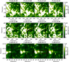 |
Fig. 1 Top panels: evolution of a network jet taken from first observation (Obs_A). The jet originates at 16:22:18 UT on 14 December 2014 from the edge of the magnetic network (panel a) with its maximum phase around 16:23:41 UT (panel c; as outlined by the red rectangle). The jet fades from view in the last phase (panel d). Middle panels: evolution of another network jet taken from second observation (Obs_ B). The jet is shown by the red rectangle. Bottom panels: evolution of one more network jet which is taken from the third observation (Obs_C). |
3.1.2 Kinematics of network jets
The space-time technique is used to evaluate the kinematics of these network jets (e.g., speed, height, and lifetime). Figure 2 shows the height-time diagram for the jet from Obs_A (first row; Fig. 1). The slit position is overplotted on the IRIS/SJI 1400 Å intensity image by red asterisk signs, which is shown in the left panel of Fig. 2. Using this path along the network jet, we used three pixels in the transverse direction to create the space-time diagram of this network jet (right panel of Fig. 2). We drew a path (white dashed line) on the space-time diagram to measure the speed of this jet, which is about 64.57 km s−1. The lifetime of the jet is 244 s; however, the jet reaches up to 4 Mm. Another network jet also appears from the same site, which indicates the concurrent energy release at the origin site.
The parameters from all 51 network jets are estimated using space-time technique; we have produced the histogram for apparent speed (panel a; Fig. 3), lifetime (panel b; Fig. 3), and length (panel c; Fig. 3). The mean speed is 140.16 km s−1 with its standard deviation of 39.41 km s−1. However, the apparent speed can vary from 50.0 to 200 km s−1. The network jet can have a lifetime that ranges from 40.0 to 250.0 s. However, the lifetime histogram of network jets predicts that the mean lifetime is 105.49 s with the standard deviation of 51.75 s. The histogram for the length of these network jets predicts the mean value of 3.16 Mm with the standard deviation of 1.18 Mm. It should also be noted that the length of these network jets can vary from 1.2 to 5.8 Mm. In addition, we also investigated the correlation between the speed and length of these jets, which is shown in panel (d). It is clearly visible that the speed and length of these jets are very positively correlated. This correlation has also been investigated by Narang et al. (2016) and they also report the positive correlation between the speed and length.
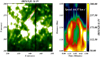 |
Fig. 2 Left panel: slit-jaw image of Si IV 1400 Å passband of IRIS during the maximum phase of the jet along the selected path (overplotted red plus signs), which is used to produce the height-time diagram. Right panel: height-timediagram of the network jet, which shows that the speed and lifetime of the network jet are ~64.57 km s−1 and 244.0 s, respectively. |
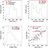 |
Fig. 3 Distribution of apparent speed (panel a), lifetime (panel b), and length (panel c) of the observed network jets. The mean speed of the network jets is 140.16 km s−1 with mean lifetime of 105.49 s. The mean length is 3.16 Mm. Panel d: the positive correlation between speed and length, as revealed by the high Pearson coefficient (R = 0.644). |
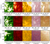 |
Fig. 4 Top (from left to right): network jet from Obs_A (first jet; Fig. 1) in IRIS/SJI Si IV 1400 Å, AIA-304 Å, AIA 171 Å, AIA 211 Å, and AIA 193 Å. Middle and bottom panels: network jet from Obs_B (second jet; Fig. 1) and from Obs_C (third jet; Fig. 1), respectively, in the same IRIS and AIA filter. It is clearly evident that network jets do not possess hot counterparts. |
3.1.3 Hot counterparts of network jets
The IRIS/SJI Si IV 1400 Å observations (Fig. 1) show the temporal evolution of three network jets (Sect. 3.1.1). The various filters from the AIA observations were used to investigate the possible hot counterparts of these network jets. However, previous works have already reported that the network jets are strictly TR phenomena and hot counterparts are not present in the solar atmosphere (e.g., Tian et al. 2014; Narang et al. 2016).
We investigated AIA 304 Å, AIA-171 Å, AIA-211 Å, and AIA-193 Å to check for the possibility of hot counterparts of the observed network jets. The top row of Fig. 4 shows the IRIS/SJI Si IV 1400 Å, AIA 304 Å, 171 Å, 211 Å, and 193 Å images for a network jet taken from Obs_A. It is clearly visible that jet is not observed in AIA filters (see red rectangular area). However, some traces of the network jet is visible in AIA 304 Å. The temperature response of the AIA 304 Å filter is very wide and it can sample some low-temperature plasma as well. The middle row shows the second jet (Obs_b) in IRIS and various AIA filters, which also predict no hot counterparts of this network jet. Similarly, the bottom row shows the network jet in different filters (AIA and IRIS) and, also similarly, no hot counterpart for this network jet is visible. Therefore, we can say thatthe network jets are clearly visible in the IRIS-SJI Si IV 1400 Å (first panel in each row; Fig. 4); however, we do not see any signature of these network jets in the hot temperature filters. We have investigated the hot temperaturefilters for all network jets (i.e., 51 network jets) and we do not see the signature of network jets in these AIA filters. Therefore, these observations predict that network jets are typically cool TR features, and our observationsare consistent with the previously reported results on this aspect (Tian et al. 2014; Narang et al. 2016).
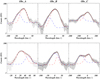 |
Fig. 5 Sample spectral profiles and their fitting from Obs_A (left column), Obs_B (middle column), and Obs_ C (right column). The black diamonds show the observed profiles, while the solid red line represents the corresponding fitting. The red dashed line shows the main Gaussian, while the blue dashed line shows the secondary Gaussian. The double-Gaussian fitting leads to very reliable fits to the observed profiles. |
3.2 Rotational nature of the network jets
The rotational motion is an important property of the jet-like structures in the solar atmosphere. On the basis of Doppler velocity/Dopplergram analysis, it has been reported that the typical coronal/chromospheric jets reveal blueshifts at one edge, while the plasma on the other side experiences redshifts (e.g., Pike & Mason 1998; Curdt & Tian 2011; Cheung et al. 2015, and references cited therein). This spatial pattern of Doppler velocity/Dopplergram reveals the rotating nature of the jet plasma column. In addition, the variations in Doppler velocity across the jet are also a signature of rotating motion of jet plasma column (e.g., Pariat et al. 2010; Young & Muglach 2014).
We utilize the optically thin TR line (Si IV 1393.75 Å) to understand the Doppler velocity pattern for these network jets. We selected Si IV 1393.75 Å spectral profiles across these network jetsfor each jet. After selecting these spectral profiles, we averaged them using a running average of two consecutive spectral profiles to increase the signal-to-noise (S/N) ratio. We found that the spectral profiles are significantly asymmetric within the vicinity of the network jets. The spectral profile appears as a double-peaked profile (bottom panel; Fig. 5) in some network jets. So, we used a double-Gaussian fitting (i.e., weak and main) to characterize the observed line. A few sample profiles along with their double-Gaussian fittings are shown in Fig. 5 from Obs_A (left column), Obs_B (middle column), and Obs_C (right column). Young & Muglach (2014) have reported the occurrence of a weak Gaussian (towards the high-velocity wing) along with the main Gaussian, which occurs in polar jets due to their very high speed. So, the secondary Gaussian basically contributes to the asymmetry of the line. The network jets are also very high-speed plasma structures within the TR, which lead to the secondary Gaussian along with main peak of Si IV 1393.75 Å. The high-velocity component of this TR line is directly attributed to the very high speed of network jets. Therefore, the secondary Gaussian of Si IV 1393.75 Å line shows the true line-of-sight (LOS) Doppler velocity of these network jets. Interestingly, we have found that the double-Gaussian fitting leads to very reliablefitting of the observed profiles (see Fig. 5). In Fig. 5, the black diamonds show the observed profile along with their errors. The overplotted solid red line represents the fitted profile. However, the red dashed line shows the main Gaussian and blue dashed line shows the secondary Gaussian. So, from all these spectral profiles, we can see that the double-Gaussian fitting leads to very reliable fitting on these observed spectral profiles.
The variation in Doppler velocity across the jet is extremely important in the context of their rotational motion. In the left panel of Fig. 6, the variations in Doppler velocity across the first jet (Obs_A, jet 1; black solid line), second jet (Obs_B, jet 2; blue line), and third jet (Obs_C, jet 3; red line) are shown. The first and second jets (jet 1 and jet 2) show that the redshift transforms into a blueshift from one edge of the jet to the other, which is a typical signature of rotational motion (e.g., Pike & Mason 1998; Curdt & Tian 2011; Cheung et al. 2015). However, jet 3 shows the increase in the Doppler velocity from one edge to its another edge. The increase or decrease in the Doppler velocity from one edge to the other also signifies the presence of rotational motion within the jet body (Young & Muglach 2014). Using this procedure, we investigated the Doppler velocity across these jets. We find that in most of the network jets, the typical spatial pattern of Doppler velocity (i.e., blueshifts on one edge and redshifts on the other) emerges. However, others have significant variations in the Doppler velocity from one edge of the network jets to the other edge. Therefore, these results successfully predict the omnipresence of the rotational motion within these network jets.
To quantify the rational motion of these network jets, we took the difference in the Doppler velocity (Δ V) between edges of any particular jet. Young & Muglach (2014) have demonstrated that the Δ V reflects the amount the rotation inherited in any particular network jet. We estimated the Δ V for each network jet to investigate their distribution. Finally, we produced the histogram of Δ V (right panel; Fig. 6), which shows the mean value of ΔV is 49.56 km s−1 with their standard deviation of 27.99 km s−1. However, the ΔV can vary from 20.0 to 100.0 km s−1. The angle between the jet’s axis and the observer (LOS direction) must be known to estimate the angular speed. However, the estimation of this angleis not possible from the used observational data. It should be noted that the angular speed is directly proportional to the ΔV; therefore, it reflects the amount of rotational motion inherited in these network jets.
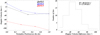 |
Fig. 6 Left panel: variation in Doppler velocity across the first jet (Obs_A; black line), second jet (Obs_B; blue line), and third jet (Obs_C; red line). Weshow the distribution of ΔV in the right panel. The mean ΔV is 49.56 km s−1 with a standard deviation of 27.99 km s−1. |
4 Discussion and conclusions
The high-resolution imaging observations of TR from IRIS reveal the ubiquitous presence of network jets. We have used three different IRIS observations of the quiet sun, which are located near the disk center. On the basis of careful inspection, 51 network jets are identified from three QS observations and used for further analysis. These 51 network jets are very well resolved and are not affected by the dynamics of other jets. The study is focused on the rotating motion of network jets along with the estimation of their other properties (speed, height, and lifetime). The mean speed, as predicted by statistical distributions of the speed, is 140.16 km s−1 with a standard deviation of 39.41 km s−1. The mean speed of network jets is very similar, as reported in previous works (e.g., Tian et al. 2014; Narang et al. 2016). However, in case of their lifetimes, we found a value that is almost double (105.49 s) that of the previously reported mean lifetime of the network jets (49.6 s; Tian et al. 2014). As mentioned above, we took only those network jets that are very well resolved in space and in the time; these criteria exclude short lifetime network jets. Therefore, our statistical distribution of the lifetime predicts a higher mean lifetime. The mean length of the network jets is 3.16 Mm with a standard deviation of 1.18 Mm. In the case of CH network jets, Tian et al. (2014) have reported that most of the network jets have lengths from 4.0 to 10.0 Mm. However, the mean length for QS network jets is smaller (3.53 Mm; Narang et al. 2016). So, the mean length for QS network jets from the present work is in good agreement with Narang et al. (2016). In addition, the apparent speed and length of these network jets are positively correlated, which is very similar to what has already been reported in previous works (Narang et al. 2016). Finally, we can say that these networks jets are very dynamic features of the solar TR, as revealed by their estimated properties.
The spectral profiles from TR were investigated extensively using space-based observations. There are some noticeable features in spectral profiles of the TR, e.g., two distinct satellites to the blue and red indicating bi-directional flows during explosive events (Dere et al. 1989), and enhanced emission in the wings above the networks (Peter 2000). In addition, Peter (2000) demonstrated that the double-Gaussian fitting yields a reliable fitting on TR spectral profiles and the secondary component is much more informative regarding the ongoing physical process. Recently, Peter (2010) reported the asymmetry in coronal extreme ultraviolet lines in the vicinity of an active region. The Si IV 1393.75 Å spectral profiles are significantly asymmetric within the observed network jets. The presence of high plasma flow at any particular jet produces the secondary component along with the main component of the line profile, which leads to the asymmetry of the spectral lines (Peter 2010). Therefore, the secondary component of the Si IV 1393.75 Å line, as observed in 51 jets in the present work, is most likely the result of high-speed plasma flows (i.e., network jets). The LOS Doppler velocity of the secondary component represents the real LOS Doppler velocity from these networks jets. The occurrence of a secondary component within the network jets is reported for first time in the present work. Our study shows that most of the network jets have opposite Doppler shifts on their edges, which is a typical signature of rotating motion of the jet plasma column (e.g., Pike & Mason 1998; Curdt & Tian 2011; Cheung et al. 2015). In addition, higher LOS Doppler velocity on one side than on the other side also predicts the rotational motion (e.g., Pariat et al. 2010; Young & Muglach 2014) in these observed jets. We have found that some network jets show this pattern, which also justifies rotational motion. So, it is clear that all the observed network jets have rotating motion. The statistical analysis predicts the mean rotational motion (Δ V) is 49.56 km s−1 with a standard deviation of 28.78 km s−1. In case of a polar jet, Young & Muglach (2014) reported that Δ V ≈ 60.0 km s1 (similar to the network jets) with a width of 4.5 arcsec. However, in the present analysis, the statistical analysis of widths shows that the mean width is 0.62 arcsec, which is almost seven times lower than the width of the polar jet. Qualitatively we can say that the angular speed of these network jets is higher than that of the usual solar jets (e.g., Shen et al. 2011; Chen et al. 2012; Young & Muglach 2014). Therefore, these network jets consist of more helical magnetic fields than the other solar jets.
In addition, the observed properties of these network jets also help us to speculate on their triggering mechanism. The magnetic reconnection between the twisted magnetic field and the pre-existing magnetic field may trigger the rotating motion (e.g., Pariat et al. 2009, 2016; Fang et al. 2014). In a numerical model Fang et al. (2014), the magnetic reconnection between twisted magnetic fields and pre-existing magnetic field can transfer the twist on newly reconnected field lines, and plasma flows along these twisted magnetic field lines. However, another numerical model (Pariat et al. 2009) is based on photospheric motion, which can transfer the twist onto the magnetic field lines and finally produce the helical jet after the magnetic reconnection due to losing the equilibrium of the flux system. The present analysis predicts the ubiquitous presence of twists within these network jets. We have also found that the network jetshave a recurrent nature (i.e., many jets are triggered at the same location) that may be the result of oscillatory magnetic reconnection, as proposed by Murray et al. (2009) and McLaughlin et al. (2012). In addition, Goodman (2014) has reported that Lorentz force-driven (i.e., magnetic acceleration) jets can have speeds of 66–397 km s−1. However, the pressure-driven jets can also achieve the maximum speed of ≈60 km s−1 (e.g., Martínez-Sykora et al. 2011). We tend to believe that the pressure-driven jet may be able to account for the speed, but not the rotational motion. Therefore, the rotating motion, recurrent nature, and apparent high speed of the observed network jets (140.16 km s−1) suggest that the magnetic reconnection is the most likely triggering mechanism in the present case. The similar aspect of the triggering mechanisms of these network jets (i.e., the recurrent nature and high apparent speed) have also been reported in some previous studies, which confirm the occurrence of magnetic reconnection in support of the formation of network jets (e.g., Tian et al. 2014; Narang et al. 2016). However, very few network jets with lower velocities (less than 60.0 km s−1) may be formed due to gas pressure acceleration (Shibata et al. 1982).
We conclude that spectral analysis predicts the omnipresence of rotational motion in the network jets, which is reported for the first time for this class of jet-like structures. The helicity (amount of rotation) is high in the observed network jets compared to the other solar jets. In addition, the magnetic reconnection/acceleration is the most likely factor leading to the formation of these network jets.
Acknowledgements
The work of P.K. and K.M. work was done in the framework of the project from the National Science Centre, Poland (NCN), Grant No. 2014/15/B/ST9/00106. IRIS is a NASA small explorer mission developed and operated by LMSAL with mission operations executed at the NASA Ames Research Center and major contributions to downlink communications funded by ESA and the Norwegian Space Centre. We also acknowledge the use of SDO/AIA observations for this study. The data provided are courtesy of NASA/SDO, LMSAL, and the AIA, EVE, and HMI science teams. A.K.S. and B.N.D. acknowledgethe RESPOND-ISRO project, and A.K.S. acknowledges the SERB-DST young scientist project grant. A.K.S. also acknowledges support by ISSI/ISSI-BJ to the team on “Pulsations in solar flares: matching observations and models”.
References
- Bohlin, J. D., Vogel, S. N., Purcell, J. D., et al. 1975, ApJ, 197, L133 [NASA ADS] [CrossRef] [Google Scholar]
- Canfield, R. C., Reardon, K. P., Leka, K. D., et al. 1996, ApJ, 464, 1016 [NASA ADS] [CrossRef] [Google Scholar]
- Chae, J., Qiu, J., Wang, H., & Goode, P. R. 1999, ApJ, 513, L75 [NASA ADS] [CrossRef] [Google Scholar]
- Chen, H.-D., Zhang, J., & Ma, S.-L. 2012, Res. Astron. Astrophys., 12, 573 [NASA ADS] [CrossRef] [Google Scholar]
- Cheung, M. C. M., De Pontieu, B., Tarbell, T. D., et al. 2015, ApJ, 801, 83 [NASA ADS] [CrossRef] [Google Scholar]
- Cirtain, J. W., Golub, L., Lundquist, L., et al. 2007, Science, 318, 1580 [NASA ADS] [CrossRef] [PubMed] [Google Scholar]
- Curdt, W., & Tian, H. 2011, A&A, 532, L9 [NASA ADS] [CrossRef] [EDP Sciences] [Google Scholar]
- De Pontieu, B., Erdélyi, R., & James, S. P. 2004, Nature, 430, 536 [NASA ADS] [CrossRef] [PubMed] [Google Scholar]
- De Pontieu, B., McIntosh, S., Hansteen, V. H., et al. 2007, PASJ, 59, S655 [Google Scholar]
- De Pontieu B., Rouppe van der Voort, L., McIntosh, S. W., et al. 2014, Science, 346, 1255732 [CrossRef] [Google Scholar]
- Dere, K. P., Bartoe, J.-D. F., & Brueckner, G. E. 1989, Sol. Phys., 123, 41 [NASA ADS] [CrossRef] [Google Scholar]
- Fang, F., Fan, Y., & McIntosh, S. W. 2014, ApJ, 789, L19 [NASA ADS] [CrossRef] [Google Scholar]
- Goodman, M. L. 2014, ApJ, 785, 87 [NASA ADS] [CrossRef] [Google Scholar]
- Kamio, S., Hara, H., Watanabe, T., et al. 2007, PASJ, 59, S757 [NASA ADS] [CrossRef] [Google Scholar]
- Kayshap, P., Srivastava, A. K., & Murawski, K. 2013a, ApJ, 763, 24 [NASA ADS] [CrossRef] [Google Scholar]
- Kayshap, P., Srivastava, A. K., Murawski, K., & Tripathi, D. 2013b, ApJ, 770, L3 [NASA ADS] [CrossRef] [Google Scholar]
- Kayshap, P., Banerjee, D., & Srivastava, A. K. 2015, Sol. Phys., 290, 2889 [NASA ADS] [CrossRef] [Google Scholar]
- Lee, E. J., Archontis, V., & Hood, A. W. 2015, ApJ, 798, L10 [NASA ADS] [CrossRef] [Google Scholar]
- Lemen, J. R., Title, A. M., Akin, D. J., et al. 2012, Sol. Phys., 275, 17 [NASA ADS] [CrossRef] [Google Scholar]
- Martínez-Sykora, J., Hansteen, V., & Moreno-Insertis, F. 2011, ApJ, 736, 9 [NASA ADS] [CrossRef] [Google Scholar]
- McLaughlin, J. A., Verth, G., Fedun, V., & Erdélyi, R. 2012, ApJ, 749, 30 [NASA ADS] [CrossRef] [Google Scholar]
- Morton, R. J., Srivastava, A. K., & Erdélyi, R. 2012, A&A, 542, A70 [NASA ADS] [CrossRef] [EDP Sciences] [Google Scholar]
- Mulay, S. M., Tripathi, D., Del Zanna, G., & Mason, H. 2016, A&A, 589, A79 [NASA ADS] [CrossRef] [EDP Sciences] [Google Scholar]
- Mulay, S. M., Del Zanna, G., & Mason, H. 2017, A&A, 598, A11 [NASA ADS] [CrossRef] [EDP Sciences] [Google Scholar]
- Murawski, K., & Zaqarashvili, T. V. 2010, A&A, 519, A8 [NASA ADS] [CrossRef] [EDP Sciences] [Google Scholar]
- Murawski, K., Srivastava, A. K., & Zaqarashvili, T. V. 2011, A&A, 535, A58 [NASA ADS] [CrossRef] [EDP Sciences] [Google Scholar]
- Murray, M. J., van Driel-Gesztelyi, L., & Baker, D. 2009, A&A, 494, 329 [NASA ADS] [CrossRef] [EDP Sciences] [Google Scholar]
- Narang, N., Arbacher, R. T., Tian, H., et al. 2016, Sol. Phys., 291, 1129 [NASA ADS] [CrossRef] [Google Scholar]
- Nishizuka, N., Shimizu, M., Nakamura, T., et al. 2008, ApJ, 683, L83 [NASA ADS] [CrossRef] [Google Scholar]
- Pariat, E., Antiochos, S. K., & DeVore, C. R. 2009, ApJ, 691, 61 [NASA ADS] [CrossRef] [Google Scholar]
- Pariat, E., Antiochos, S. K., & DeVore, C. R. 2010, ApJ, 714, 1762 [NASA ADS] [CrossRef] [Google Scholar]
- Pariat, E., Dalmasse, K., DeVore, C. R., Antiochos, S. K., & Karpen, J. T. 2016, A&A, 596, A36 [NASA ADS] [CrossRef] [EDP Sciences] [Google Scholar]
- Pereira, T. M. D., De Pontieu, B., Carlsson, M., et al. 2014, ApJ, 792, L15 [NASA ADS] [CrossRef] [Google Scholar]
- Peter, H. 2000, A&A, 360, 761 [NASA ADS] [Google Scholar]
- Peter, H. 2010, A&A, 521, A51 [NASA ADS] [CrossRef] [EDP Sciences] [Google Scholar]
- Pike, C. D., & Mason, H. E. 1998, Sol. Phys., 182, 333 [NASA ADS] [CrossRef] [Google Scholar]
- Rao, Y. K., Srivastava, A. K., Doyle, J. G., & Dwivedi, B. N. 2017, MNRAS, 470, 2449 [NASA ADS] [CrossRef] [Google Scholar]
- Raouafi, N. E., Patsourakos, S., Pariat, E., et al. 2016, Space Sci. Rev., 201, 1 [NASA ADS] [CrossRef] [Google Scholar]
- Schmieder, B., Shibata, K., van Driel-Gesztelyi, L., & Freeland, S. 1995, Sol. Phys., 156, 245 [NASA ADS] [CrossRef] [MathSciNet] [Google Scholar]
- Shen, Y., Liu, Y., Su, J., & Ibrahim, A. 2011, ApJ, 735, L43 [NASA ADS] [CrossRef] [Google Scholar]
- Shibata, K., Nishikawa, T., Kitai, R., & Suematsu, Y. 1982, Sol. Phys., 77, 121 [NASA ADS] [CrossRef] [Google Scholar]
- Shibata, K., Nakamura, T., Matsumoto, T., et al. 2007, Science, 318, 1591 [NASA ADS] [CrossRef] [Google Scholar]
- Srivastava, A. K., & Murawski, K. 2011, A&A, 534, A62 [NASA ADS] [CrossRef] [EDP Sciences] [Google Scholar]
- Takasao, S., Isobe, H., & Shibata, K. 2013, PASJ, 65, 62 [NASA ADS] [CrossRef] [Google Scholar]
- Tian, H., DeLuca, E. E., Cranmer, S. R., et al. 2014, Science, 346, 1255711 [Google Scholar]
- Wilhelm, K. 2000, A&A, 360, 351 [NASA ADS] [Google Scholar]
- Yokoyama, T.,& Shibata, K. 1995, Nature, 375, 42 [NASA ADS] [CrossRef] [Google Scholar]
- Yokoyama, T.,& Shibata, K. 1996, PASJ, 48, 353 [NASA ADS] [CrossRef] [Google Scholar]
- Young, P. R., & Muglach, K. 2014, PASJ, 66, S12 [NASA ADS] [CrossRef] [Google Scholar]
All Tables
Date and time, field of view (FOV), and exposure time (in seconds) for SJI and raster for all three sets of observations.
All Figures
|
Fig. 1 Top panels: evolution of a network jet taken from first observation (Obs_A). The jet originates at 16:22:18 UT on 14 December 2014 from the edge of the magnetic network (panel a) with its maximum phase around 16:23:41 UT (panel c; as outlined by the red rectangle). The jet fades from view in the last phase (panel d). Middle panels: evolution of another network jet taken from second observation (Obs_ B). The jet is shown by the red rectangle. Bottom panels: evolution of one more network jet which is taken from the third observation (Obs_C). |
| In the text | |
|
Fig. 2 Left panel: slit-jaw image of Si IV 1400 Å passband of IRIS during the maximum phase of the jet along the selected path (overplotted red plus signs), which is used to produce the height-time diagram. Right panel: height-timediagram of the network jet, which shows that the speed and lifetime of the network jet are ~64.57 km s−1 and 244.0 s, respectively. |
| In the text | |
|
Fig. 3 Distribution of apparent speed (panel a), lifetime (panel b), and length (panel c) of the observed network jets. The mean speed of the network jets is 140.16 km s−1 with mean lifetime of 105.49 s. The mean length is 3.16 Mm. Panel d: the positive correlation between speed and length, as revealed by the high Pearson coefficient (R = 0.644). |
| In the text | |
|
Fig. 4 Top (from left to right): network jet from Obs_A (first jet; Fig. 1) in IRIS/SJI Si IV 1400 Å, AIA-304 Å, AIA 171 Å, AIA 211 Å, and AIA 193 Å. Middle and bottom panels: network jet from Obs_B (second jet; Fig. 1) and from Obs_C (third jet; Fig. 1), respectively, in the same IRIS and AIA filter. It is clearly evident that network jets do not possess hot counterparts. |
| In the text | |
|
Fig. 5 Sample spectral profiles and their fitting from Obs_A (left column), Obs_B (middle column), and Obs_ C (right column). The black diamonds show the observed profiles, while the solid red line represents the corresponding fitting. The red dashed line shows the main Gaussian, while the blue dashed line shows the secondary Gaussian. The double-Gaussian fitting leads to very reliable fits to the observed profiles. |
| In the text | |
|
Fig. 6 Left panel: variation in Doppler velocity across the first jet (Obs_A; black line), second jet (Obs_B; blue line), and third jet (Obs_C; red line). Weshow the distribution of ΔV in the right panel. The mean ΔV is 49.56 km s−1 with a standard deviation of 27.99 km s−1. |
| In the text | |
Current usage metrics show cumulative count of Article Views (full-text article views including HTML views, PDF and ePub downloads, according to the available data) and Abstracts Views on Vision4Press platform.
Data correspond to usage on the plateform after 2015. The current usage metrics is available 48-96 hours after online publication and is updated daily on week days.
Initial download of the metrics may take a while.