| Issue |
A&A
Volume 615, July 2018
|
|
|---|---|---|
| Article Number | A92 | |
| Number of page(s) | 11 | |
| Section | Astronomical instrumentation | |
| DOI | https://doi.org/10.1051/0004-6361/201832973 | |
| Published online | 19 July 2018 | |
Astrometric and photometric accuracies in high contrast imaging: The SPHERE speckle calibration tool (SpeCal)⋆
1
Lesia, Observatoire de Paris, PSL Research University, CNRS, Sorbonne Universités, Univ. Paris Diderot, UPMC Univ. Paris 06, Sorbonne Paris Cité, 5 place Jules Janssen, 92190
Meudon, France
e-mail: This email address is being protected from spambots. You need JavaScript enabled to view it.
2
INAF – Osservatorio Astronomico di Padova, Vicolo della Osservatorio 5, 35122
Padova, Italy
3
INCT, Universidad De Atacama, calle Copayapu 485, Copiapó, Atacama, Chile
4
Université Grenoble Alpes, CNRS, IPAG, 38000
Grenoble, France
5
Aix-Marseille Université, CNRS, LAM (Laboratoire d’Astrophysique de Marseille) UMR 7326, 13388
Marseille, France
6
CRAL, UMR 5574, CNRS, Université de Lyon, Ecole Normale Supérieure de Lyon, 46 Allée d’Italie, 69364
Lyon Cedex 07, France
7
Max-Planck-Institut für Astronomie, Königstuhl 17, 69117
Heidelberg, Germany
8
Institute for Astronomy, University of Edinburgh, Blackford Hill, Edinburgh EH9 3HJ, UK
9
Department of Astronomy, Stockholm University, 106 91
Stockholm, Sweden
10
Université Côte d’Azur, OCA, CNRS, Lagrange, France
11
Universidad de Chile, Camino el Observatorio 1515, Santiago, Chile
12
Núcleo de Astronomía, Facultad de Ingeniería, Universidad Diego Portales, Av. Ejercito 441, Santiago, Chile
13
Millenium Nucleus “Protoplanetary Disks in ALMA Early Science”, Valparaiso, Chile
14
Geneva Observatory, University of Geneva, Chemin des Mailettes 51, 1290
Versoix, Switzerland
Received:
7
March
2018
Accepted:
21
April
2018
Abstract
Context. The consortium of the Spectro-Polarimetric High-contrast Exoplanet REsearch installed at the Very Large Telescope (SPHERE/VLT) has been operating its guaranteed observation time (260 nights over five years) since February 2015. The main part of this time (200 nights) is dedicated to the detection and characterization of young and giant exoplanets on wide orbits.
Aims. The large amount of data must be uniformly processed so that accurate and homogeneous measurements of photometry and astrometry can be obtained for any source in the field.
Methods. To complement the European Southern Observatory pipeline, the SPHERE consortium developed a dedicated piece of software to process the data. First, the software corrects for instrumental artifacts. Then, it uses the speckle calibration tool (SpeCal) to minimize the stellar light halo that prevents us from detecting faint sources like exoplanets or circumstellar disks. SpeCal is meant to extract the astrometry and photometry of detected point-like sources (exoplanets, brown dwarfs, or background sources). SpeCal was intensively tested to ensure the consistency of all reduced images (cADI, Loci, TLoci, PCA, and others) for any SPHERE observing strategy (ADI, SDI, ASDI as well as the accuracy of the astrometry and photometry of detected point-like sources.
Results. SpeCal is robust, user friendly, and efficient at detecting and characterizing point-like sources in high contrast images. It is used to process all SPHERE data systematically, and its outputs have been used for most of the SPHERE consortium papers to date. SpeCal is also a useful framework to compare different algorithms using various sets of data (different observing modes and conditions). Finally, our tests show that the extracted astrometry and photometry are accurate and not biased.
Key words: instrumentation: high angular resolution / methods: observational / techniques: image processing / planets and satellites: detection
Based on observations collected at the European Organisation for Astronomical Research in the Southern Hemisphere under ESO programme 097.C-0865.
e-mail: This email address is being protected from spambots. You need JavaScript enabled to view it.
© ESO 2018
 Open Access article, published by EDP Sciences, under the terms of the Creative Commons Attribution License (http://creativecommons.org/licenses/by/4.0), which permits unrestricted use, distribution, and reproduction in any medium, provided the original work is properly cited.
1. Introduction
The Spectro-Polarimetric High-contrast Exoplanet REsearch (SPHERE; Beuzit et al. 2008) is a facility-class instrument at the Very Large Telescope (VLT) dedicated to directly imaging and spectroscopically characterizing exoplanets and circumstellar disks. It combines a high-order adaptive-optics system with diverse coronagraphs. Three instruments are available: an infrared dual-band imager (IRDIS, Dohlen et al. 2008), an infrared integral field spectrometer (IFS, Claudi et al. 2008), and a visible imaging polarimeter (Zimpol, Thalmann et al. 2008).
Since first light in May 2014, SPHERE has been performing well in all observational modes, enabling numerous follow-up studies of known sub-stellar companions to stars and circumstellar disks as well as new discoveries (e.g., Boccaletti et al. 2015; de Boer et al. 2016; Ginski et al. 2016; Lagrange et al. 2016; Maire et al. 2016a, 2017; Mesa et al. 2016, 2017; Perrot et al. 2016; Vigan et al. 2016; Zurlo et al. 2016; Chauvin et al. 2017; Bonnefoy et al. 2017; Feldt et al. 2017; Samland et al. 2017). The good performance to date results from the stability of the instrument over time and a dedicated and sophisticated software for data reduction.
The SPHERE reduction software uses the data reduction handling pipeline (DRH, Pavlov et al. 2008) that was delivered to ESO with the instrument as well as upgraded tools optimized using the first SPHERE data to derive accurate spectrophotometric and astrometric calibrations (Mesa et al. 2015; Maire et al. 2016b). The software that is implemented at the SPHERE data center (Delorme et al. 2017a) first assembles tens to thousands of images or spectra into calibrated datacubes, removing or correcting for instrumental artifacts. This includes image processing steps such as flat-fielding, bad pixels, background, frame selection, anamorphism correction, true north alignment, frame centring, and spectral transmission. The outputs of these first steps are temporal and spectral sequences of images organized in datacubes with four dimensions hereafter: coronagraphic images and the associated point-spread functions (PSF). Then, the software uses the speckle calibration tool (SpeCal) written in the IDL language and described in this paper. SpeCal was developed in the context of the SpHere INfrared survey of Exoplanets (SHINE), which is the main part of the SPHERE guaranteed observation time (GTO) and is now used to process all SPHERE data obtained with IRDIS and IFS systematically. SpeCal uses data processing algorithms proposed in the literature. Data from the Zurich imaging polarimeter (ZIMPOL) will be implemented in the future.
In Sect. 2, we describe the algorithms that SpeCal uses to optimize the exoplanet detection, while in Sect. 3 we explain how SpeCal algorithms estimate the astrometry and photometry of point-like sources like exoplanets or brown dwarfs. To address the accuracies of the data reduction in terms of astrometry and photometry we use SpeCal to reduce two sequences recorded with IRDIS (Sect. 4) and IFS (Sect. 5) during the SPHERE guaranteed time observations.
2. Calibration of the speckle pattern
2.1. Differential imaging strategies
Current high contrast imaging instruments dedicated to exoplanet detection combine an adaptive optics system to compensate for the atmospheric turbulence and coronagraphs to attenuate the flux of the central bright source (i.e. the star). Because the adaptive optics system is not perfect and because of aberrations in the optics of the telescope and instrument, part of the stellar light reaches the science detector, creating spatial interference patterns called speckles. The speckles mimic images of off-axis point-like sources, especially in narrow band filters. Other factors let stellar light go through the coronagraph preventing the detection of faint sources in the raw data: chromatism of the coronagraph, atmospheric dispersion, diffraction effects from the secondary mirror and from spiders, low wind effect, and so on. Hereafter, for convenience, the stellar speckle pattern will refer to any type of stellar light that reaches the detector even if it is not in the form of speckles.
Strategies that are routinely used to discriminate exoplanet images from the stellar speckle pattern include angular differential imaging (ADI, Marois et al. 2006), dual-band imaging, and spectral differential imaging (SDI, Rosenthal et al. 1996; Racine et al. 1999; Marois et al. 2004; Thatte et al. 2007), reference differential imaging (RDI, Beuzit et al. 1997), and polarization differential imaging (PDI, Baba & Murakami 2003; Baba et al. 2005). Each strategy relies on specific assumptions about the speckle pattern, and the efficiency of extracting the planet signal from the speckle pattern is directly related to the strengths and limitations of these assumptions. When using ADI, we assume most of the optical aberrations come from planes that are optically conjugated to the pupil plane and remain static in the course of the observation. Keeping the pupil orientation fixed (pupil tracking mode), we record a sequence of images that show a stable speckle pattern while the field of view, including an off-axis exoplanet image, rotates around the central star. Using dual-band imaging, we assume the spectrum of the star (and so, the speckles) is different from the exoplanet spectrum. Using SDI, we assume the speckles are induced by an achromatic optical path difference in a pupil plane so that we can predict the evolution of the phase aberrations that induce the speckles with wavelength. Using RDI, we observe several similar stars with a similar instrumental set-up assuming the speckle pattern is stable in time. Finally, the PDI technique assumes that, unlike the star light, the light coming from the planet is polarized. For each strategy, several algorithms exist to process the data.
The SPHERE instrument can record coronagraphic images simultaneously in two spectral filters using the IRDIS subsystem for dual-band imaging (Vigan et al. 2010) or in 39 narrow spectral channels using the IFS for SDI (Zurlo et al. 2014; Mesa et al. 2015). During the observations, ADI, dual-band imaging, and SDI can be used so that the SPHERE instrument records fourdimensional datacubes, called I(x, y, θ, λ): two spatial dimensions (x, y, sky coordinates), one angular dimension (θ, orientation with respect to the north direction, which evolves with time in pupil tracking mode), and one spectral dimension (λ, wavelength). In the rest of the paper, we use “spectral channel” to refer to the spectral dimension, and “angular channel” to refer to the angular dimension. Also, we use SDI for both SDI and dual-band imaging.
The SpeCal tool was developed so that all the SHINE SPHERE GTO data can be uniformly processed. We remind readers that this tool uses data processing techniques that were previously proposed in the literature. The interest of the tool is that all these techniques have been tested on several datasets to ensure that all the products are consistent (contrast curves, measurements of astrometry, and photometry of detected pointlike sources). SpeCal can process data recorded using ADI, SDI, RDI, or the combination of ADI and SDI that is called ASDI hereafter (see Table 1). When SDI or ASDI is chosen, the frames I(x, y, θ, λ) are spatially scaled with wavelength to compensate for the spectral dispersion of the speckle position and size, the reference wavelength being the shortest one. The resulting frames are called I s(x, y, θ, λ). The scaling changes the spatial sampling. An inverse scaling is performed at the end of the data processing. The ASDI option usually minimizes the speckle pattern more efficiently but it can strongly bias the photometry of the objects that are detected, as demonstrated in Maire et al. (2014) and Rameau et al. (2015).
Acronyms of the strategies of observation.
Numerous algorithms were proposed to minimize the speckle pattern in coronagraphic images so that point-like sources (e.g., exoplanets) or extended sources (e.g., circumstellar disks) can be detected. SpeCal offers several algorithms depending on the observing strategy: classical ADI (cADI, Marois et al. 2006), classical reference differential imaging (cRDI), subtraction of a radial profile (radPro), locally optimized combination of images (Loci, Lafrenière et al. 2007), LociRDI, template-Loci (TLoci, Marois et al. 2014), principal component analysis (PCA, Soummer et al. 2012; Amara & Quanz 2012), and classical averaging with no subtraction (ClasImg). The objective of each algorithm, except ClasImg, is the determination of one speckle pattern A(x, y, θ, λ) that is then subtracted from I(x, y, θ, λ) to obtain a datacube R(x, y, θ, λ) where the stellar intensity is reduced: (1)
(1)
The pattern A can be a function of the spectral dimension, of the angular dimension, and of the sky coordinates.
In the ADI cases, once the A pattern is subtracted, all frames of R are rotated to align their north axis. In the SDI case, the R frames are spatially scaled to recover the initial sampling. In the ASDI case, the R frames are both spatially scaled and rotated. Then, the frames are mean-combined to sum up the offaxis source signal. The result is a datacube Ifinal(x, y, λ). SpeCal also uses a median combination of the R frames. Hence, there are two final images for each spectral channel.
The following sections describe how SpeCal calculates the A pattern for each algorithm, the acronyms for which are given in Table 2.
Acronyms and names of algorithms used to process the data recorded using a given strategy of observation (third column).
2.2. Classical averaging
SpeCal can provide the average and median combinations of the rotated R frames using A = 0. This algorithm (ClasIm) can be useful to optimize the signal-to-noise (S/N) ratio of detections in parts of the image that are dominated by background instead of speckles.
2.3. cADI
In classical ADI, SpeCal averages the cube of frames over the angular dimension for each spectral channel (λ): (2)
(2)
Equation (1) is applied and the R frames are rotated and then averaged to produce one final image Ifinal,a per spectral channel.
SpeCal can also remove the median of the frames instead of the average: (3)
(3)
Then, it uses Am in Eq. (1), rotates the R frames, and then applies a median combination. The final image Ifinal,m is less sensitive than Ifinal,a to uncorrected hot or bad pixels. It is however harder to accurately retrieve the photometry of a detected offaxis source from Ifinal,m than from Ifinal,a (Sect. 3).
2.4. cRDI
The reference differential imaging (RDI) is especially useful to obtain images of extended sources like circumstellar disks or to probe small angular separations to the star because it is not subject to self-subtraction unlike the other algorithms. The classical RDI (cRDI) is similar to cADI but it uses N reference frames IR(x, y, n, λ) to derive the speckle pattern A, where n = 1 … N. These reference frames are images of stars other than the one of interest (IR ≠ I). The resulting A pattern is (4)
(4)
2.5. Subtraction of a radial profile
For detecting and studying extended sources, SpeCal proposes the radPro algorithm that first works out the average of the datacube over the angular dimension (Eq. (2)). Then, it calculates the azimuthally averaged profile in rings of one pixel width. Finally, the A pattern is the centro-symmetrical image that is derived from this profile.
2.6. Loci
The SpeCal Loci algorithm is described in Lafrenière et al. (2007). For a given θ, a given λ, and a given region in the field (blue in Fig. 1), the algorithm calculates the linear combination of the other frames Is(x, y, θ′, λ′) (θ′ ≠ and λ′ ≠ λ in ASDI) to build A(x, y, θ, λ) that minimizes |R| (Eq. (1)) in the region of interest. In addition to the algorithm of Lafrenière et al. (2007), we impose the coefficients of the linear combination to be positive. Conversely to Lafrenière et al. (2007), the region of interest where A is applied and the region of optimization from which A is derived are the same in SpeCal. They are defined using:
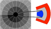 |
Fig. 1. Loci and TLoci regions of interest (left figure and central blue region in the right figure) and TLoci optimizing region (exterior red region in the right figure). |
-
the radial width of the region (dr in Lafrenière et al. 2007);
-
the number of PSFs inside the region (NA in Lafrenière et al. 2007).
We use different parameters to Lafrenière et al. (2007) to select the frames that are used in the linear combination. Consider the frame Is(x, y, θ, λ) (ASDI case, Sect. 2.1). First, we assume the image Ip of a putative off-axis source in Is is the two-dimensional Gaussian function with the full width half-maximum (FWHM) estimated from the recorded PSF (see Sect. 2.10.1). If the source is in the region centered on (x0, y0) in Is(x, y, θ, λ), it is angularly shifted by sθ = r0 (θi − θ) and radially shifted by sr = r0 (1 − λ/λj) in Is(x, y, θi, λj), where  is the angular separation from the star in FWHM unit. If only Is(x, y, θi, λj) was used to build A, the normalized intensity of the off-axis source integrated within a disk of one-FWHM diameter in the frame R would be
 (5)
(5)
using x′ = x − x0, y′ = y − y0 and  . Then,
 (6)
(6)
Using the radial and angular shifts sr and sθ of Is(x, y, θi, λj), we find (7)
(7)
where α equals  , and erf is the error function, and
 (8)
(8)
Here, we assume the angular motion is linear, which is a good assumption because E(s) quickly decreases. The function τ′ goes from 0 (θ = θi and λ = λj, total self-subtraction) to 1 (no self-subtraction). In SpeCal, we set a parameter τ that can be linked to the minimum motion δmin of the putative off-axis source in Lafrenière et al. (2007). If τ′ is smaller than τ, the frame Is(x, y, θi, λj) is rejected. Doing so for each θi and λj, we obtain a series of frames {Is} that individually leave at least τ times the initial flux of the putative source in the R(x, y, θ, λ). Then, we select from {Is} the N most correlated frames (N is adjustable) to Is(x, y, θ, λ) in the considered region. We obtain the linear combination of the N frames (i.e., the A pattern) that minimizes the residual energy in this region using the bounded-variables least-squares algorithm by Lawson & Hanson (1995). Finally, as the coefficients of the linear combination are positive, the flux of the putative source in the final image Ifinal is at least τ times the initial flux for any region.
The Loci algorithm can be used to reduce ADI, SDI, or ASDI data. In the ADI case, the Loci A pattern that is worked out for a given frame I(x, y, θ, λ) uses the other frames taken in the same spectral channel only. In the SDI case, it uses the frames taken with the same angle θ only. Finally, in the ASDI case, all frames are spatially scaled with wavelength, and they are all used to determine the A pattern.
2.7. TLoci
The SpeCal TLoci algorithm is derived from the one described in Galicher & Marois (2011) and Marois et al. (2014) assuming a flat planet spectrum in contrast. The parameters that are used to select the frames (τ and N) and to describe the regions of interest (dr and NA) where the A pattern is applied (blue region in Fig. 1) are the same as for the Loci case (Sect. 2.6). The difference from Loci is the region where A is optimized (red region). In SpeCal, the gap between this region and the region of interest is set to 0.5 FWHM. Hence, the optimizing region is close enough to the region of interest so that A is efficiently optimized, and the optimizing region is far enough from the region of interest so that the flux of a source in the latter does not bias the linear combination. Moreover, the internal radii of the two regions are the same in SpeCal. Finally, an additional parameter sets the radial width of the optimizing region. As for Loci, TLoci can be associated to ADI, SDI, and ASDI.
2.8. LociRDI
A reference differential imaging algorithm using Loci is also implemented in SpeCal. It works as described in Sect. 2.6 but the frames that are used to build A are reference frames as in the cRDI case (Sect. 2.4).
2.9. PCA
For historical reasons, two PCA algorithms are implemented in SpeCal. The first version can be applied on IRDIS or IFS data using the ADI or ASDI options. This algorithm follows the equation of Soummer et al. (2012). For each frame I(x, y, θ, λ), we subtract its average over the field of view: (9)
(9)
In the ADI case, the principal components are calculated for each spectral channel independently. Each frame Iz(x, y, θ, λ) is then projected onto the N first components to obtain the A pattern that is used in Eq. (1), replacing I with Iz. The N parameter is called “number of modes” hereafter. Finally, the averages that were removed (Eq. (9)) are added back to obtain the R frames of Eq. (1). In the ASDI case, the algorithm is the same but it works on Is instead of I. We note that here there is no frame selection to minimize the self-subtraction of point-like sources when deriving the principal components.
The second version of PCA that is implemented in SpeCal is very similar to the first one but it can be applied on IFS data using the ASDI option only (Mesa et al. 2015). The two PCA versions were tested on a large amount of SPHERE data and they provide a very similar performance.
2.10. Common outputs
2.10.1. Model of unsaturated PSF
SpeCal produces common outputs whatever the chosen algorithm. First, it records the final images Ifinal normalized to the estimated maximum of an unsaturated non-coronagraphic stellar image with the same exposure time. Hence, the values of the pixels in Ifinal give the contrast ratio to the star maximum. For each spectral channel, the maximum β of the stellar non-coronagraphic image is derived from the best fit of the input PSFs by the function (10)
(10)
where α is the background level, β is the star maximum, γ and η are related to the spatial extension of the PSF (and to FWHM), and (xPSF, yPSF) give the center of the PSF. All these parameters are fitted accounting for the photon noise in the provided PSF images. The SPHERE PSFs are usually close to two-dimensional Gaussian functions (η = 2) but can deviate from them. In the context of SHINE, PSFs are usually recorded before and after the coronagraphic sequence. SpeCal calculates the best fit to each of the PSFs (~50 × 50 pixels) and runs two tests on the time series of fitted parameters. First, it works out the average and standard deviation of the normalization factor β over time, records the two values, and sends a warning if the flux of the star β varies by more than 20% between distinct PSF observations of the target. Then, it sends a warning if the background level α is larger than 10% of β. These values (10% and 20%) were defined as quality requirements based on our experience with the instrument and the analysis of hundreds of datasets. Finally, SpeCal estimates and records the PSF FWHM.
2.10.2. Calibration of photometry
For algorithms that bias the photometry of off-axis sources, SpeCal estimates the throughput of the technique at each position in the field. For cADI, radPro, and PCA, SpeCal creates a datacube of fake planets that are on a linear spiral centered on the star (one planet per 2 FWHM). For each planet, we use the recorded PSF and its flux equals ten times the local residual flux in Ifinal. The fake planet datacube is added to the datacube I(x, y, θ, λ). Then, SpeCal combines the frames as the I(x, y, θ, λ) were combined to get Ifinal. For each planet, the ratio of the flux in the resulting image to the flux of the fake planet is calculated to obtain the 1D-throughput as a function of the angular separation. For Loci and TLoci, the throughput τR is estimated in each frame R as the average of all τ′ of Eq. (7), weighting E(sθ) and E(sr) by the coefficients used to obtain Ifinal. We average all τR to obtain the 1D-throughput as a function of the angular separation. Finally, the throughput map T is the centro-symmetrical image created from the 1D-throughput. SpeCal also calculates the throughput-corrected final image Ifinal/T.
2.10.3. S/N and detection maps
For each spectral channel, the image Ifinal/T is divided into annulii of 0.5 FWHM width. Then, in each annulus (i.e., at each angular separation), we calculate the standard deviation that is set to be the 1 σ contrast. S/N maps are also created. Each pixel gives the ratio of the flux in Ifinal/T to the standard deviation of Ifinal/T calculated in annulii of 1 FWHM centered on the star. This correction is valid only for point-like sources. For example, this correction is not valid for an extended source like a disk. Finally, SpeCal also provides local detection maps giving the local standard deviation in boxes of 2 FWHM radial size and of a total area of 5 FWHM2.
3. Astrometry and photometry of point-like sources
All algorithms, except RDI and ClasImg, distort the image of an off-axis point-like source in Ifinal (Sect. 3.1). Thus, the estimation of the position and flux of such a source cannot be done directly from Ifinal (Marois et al. 2010; Lagrange et al. 2010; Galicher & Marois 2011; Maire et al. 2014; Rameau et al. 2015). However, SpeCal can fit a model of an off-axis source image to the detected source in Ifinal (Sect. 3.2), or it can inject a negative point-like source into the initial datacube I and adjust the position and flux of this negative source to locally minimize the flux in Ifinal (Sect. 3.3).
3.1. Planet image
Say there is a planet whose intensity is described by Ip(x, y, θ, λ) whereas the stellar intensity is I*(x, y, θ, λ). The A pattern is derived from the cube (11)
(11)
and part of the A pattern is composed of planet signal. For example, when using cADI, Loci, TLoci, or radPro on ADI, SDI, or ASDI data, the A pattern can be expressed as (12)
(12)
 (13)
(13)
 (14)
(14)
where coefficients ci,j are real numbers that can be a function of (x, y), and (15)
(15)
Hence, the A pattern is contaminated by planet signal and, when subtracting the A pattern from the initial frames I, part of the planet signal self-subtracts. The R frames is then (16)
(16)
where all terms depend on x, y, θ, and λ. A perfect algorithm – that does not exist – would be such that A* = I* and Ap = 0.
As the planet image moves in the field from one frame to another (radially for SDI or azimuthally for ADI), the subtracted signal is shifted with respect to the astrophysical position of the planet. This results in a positive-negative pattern of the planet in each frame of R and as a consequence in the final image Ifinal (left in Fig. 2). This pattern is not always centered on the planet position. The distortions of the planet image can be minimized by carefully selecting the frames that are used to build A (so that Ap → 0) but it usually reduces the efficiency of the speckle attenuation at the same time (increasing |I* − A*|). In the case of PCA algorithms, I(x, y, θi, λi) in Eq. (12) is replaced by the principal components, which are also contaminated by the planet signal.
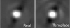 |
Fig. 2. Real (left) and estimated (right) images of an off-axis source in an ADI reduced image showing the negative wings due to self-subtraction of the planet flux. |
3.2. Model of planet images
The first way of extracting the astrometry and the photometry of an off-axis point-like source like a planet in an ADI, SDI, or ASDI reduced image consists of building a model of the planet image (Galicher & Marois 2011). First, we estimate the position of the detected source in Ifinal with a pixel accuracy. Then, we use the measured stellar PSF to build a sequence of frames Ifp(x, y, θ, λ) with only one fake planet image at the rough position accounting for the field-of-view rotation. We do not account for the smearing that affects images. This effect may be non-negligible at the edges of the IRDIS images if the field-of-view rotation is fast and the exposures are long, which is rare. We combine the frames Ifp in the same way the frames I were combined using the same ci,j and we get an estimation of Ap (Eq. (15)). Rotating (ADI case), spatially scaling (SDI case), and averaging the frames result in a model of the planet image (right in Fig. 2). The planet image has negative wings due to the self-subtraction of the planet flux (Sect. 3.1).
Then, the flux and the position of this synthetic image are adjusted to best fit the real planet image within a disk of diameter 3 FWHM so that it includes the positive and the negative parts of the image. The optimization is done using Ifinal, which is derived from the average of the R frames after rotation and spatial scaling (and not the one obtained using the median-combination that does not preserve linearity). Rigorously, we should calculate the synthetic image each time we test a new planet position. To optimize computation time, we shift the synthetic planet image that was obtained with the rough position. We noticed no significant difference as long as the shifts are smaller than ~1 FWHM.
Once the optimization is done, we look for the excursion of each parameter that increases the minimum residual level by a factor of 1.15. We set these excursions to be the 1 σ accuracies due to the fitting errors in the SpeCal outputs. The value of 1.15 is empirical but it was tested on numerous cases (high or low S/N detection, strong or weak negative wings, Loci, TLoci, PCA, and others). Another SpeCal output is the standard deviation in time of the averaged flux in the coronagraphic images. To avoid saturated parts of the images and background dominated parts, the averaged flux is calculated inside an annulus centered on the star and going from 30 pixels to 50 pixels in radius.
SpeCal can use this technique to extract astrometry and spectro-photometry in images obtained with any algorithm (cADI/radPro/Loci/TLoci/PCA/averaging) and any of ADI, SDI, or ASDI. It can also be used on cRDI, LociRDI, and ClasImg final images. In these cases, the planet image model is the stellar PSF shifted at the position of the detection with no negative wings as the Ap pattern is null (classical fit of a non-coronagraphic image).
3.3. Negative planets
Another technique – the fake negative planet – (Lagrange et al. 2010; Chauvin et al. 2012) is implemented in SpeCal to retrieve the photometry and astrometry of point-like sources. First, we build the sequence of frames Ifp with the fake planet only, as done in Sect. 3.2. Then, we subtract this datacube from the initial data I. We apply the algorithm and get the final image from the I − Ifp frames. In this final image, we measure the standard deviation of the residual intensity inside a disk of 3 FWHM diameter centered on the rough position of the detected planet. Modifying the fake planet position and flux, we minimize the residual intensity. The uncertainties on the best values are estimated as the ones in Sect. 3.2. The negative planet technique is more time-consuming than the model of planet image technique because it calculates the ci,j for all the tested fake planet positions and fluxes. It is, however, needed in some cases for which the model of planet image technique is biased (Sect. 4.2).
4. Reduction of IRDIS data
In Sects. 4 and 5, we use SpeCal to reduce two datasets as examples. In Sect. 4, we consider one sequence recorded during the SPHERE GTO on 2016 September 16 observing HIP2578 in IRDIS H2/H3 mode. There are 80 images of 64 s exposure time and the field of view rotates by 31.5°. The seeing was about 0.5 arcsec and the average wind speed was 7.4 m s−1.
All algorithms are applied on the same datacube provided by the first part of the SPHERE pipeline (background, flat-fielding, bad pixels, registration, wavelength calibration, astrometric calibration; Pavlov et al. 2008; Zurlo et al. 2014; Maire et al. 2016b). The datacube is a 1024 × 1024 × 80 × 2 array. The last dimension stands for the two spectral channels (H2 and H3). We also added three fake planets to the data (see Table 3) using the recorded stellar PSFs. We chose the position and the flux to have three typical cases. Planets 1 and 2 are in the speckle dominated part of the image, planet 2 being surrounded by brighter speckles. Planet 3 is in a region dominated by the background and not by speckles.
Separations to the central star in pixels towards east (ΔRA) and north (ΔDec), angular separations in mas and flux ratio with respect to the star (C) for each fake planet added to the IRDIS data.
4.1. Calibration of the speckle pattern
We apply several algorithms to the two spectral channels independently (no use of SDI) and we show the average of the two final images in Fig. 3 for cADI, TLoci, Loci, and two PCA (5 and 10 modes). Images are corrected from the technique throughput T (self-subtraction of a putative planet, Sect. 2.10.2) and from the coronagraph transmission. All images provide similar sensitivities except for cADI, which is less efficient inside the AO correction area that is dominated by speckles. The three fake planets are well detected in all images. The corresponding 5σ contrast curves are plotted in Figs. 4 (H2) and 5 (H3), where the three planets are represented by plus symbols. The curves are corrected for the throughput T of each technique and from the coronagraph transmission (Guerri et al. 2011). The latter is a function of angular separation and it was calibrated at the telescope and via numerical simulations. We also overplot the contrast before any a posteriori speckle minimization with a dotted line (ClasImg). The utility of a speckle calibration during the data processing is obvious since none of the planets are detected in the images with no subtraction (ClasImg). In this example, all the algorithms except cADI give similar performances in terms of contrast level. For some sequences, one algorithm reaches better contrast levels but there is no algorithm in SpeCal that is always better than the others.
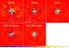 |
Fig. 3. IRDIS example: final images using cADI, Tloci, Loci, PCA (5 and 10 modes). Images are corrected from the technique throughput and from the coronagraph transmission. The color scale, which is the same for all images, shows the contrast to the star ratio. The spatial scale is the same for all images. |
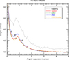 |
Fig. 4. Contrast curves at 5 σ before (ClasImg) and after minimization of the stellar light using different algorithms (cADI, Tloci, Loci, PCA 5 modes) on H2 data. The curves are corrected from the technique attenuation and from the coronagraph transmission. The fake planets are represented by plus symbols. |
The small sample statistic bias (Mawet et al. 2014) that mainly affects separations at less than 0.2″ will be implemented in the next version of the tool. This correction will affect all the algorithm reductions the same way.
4.2. Measurements of astrometry and photometry
We extract the astrometry and photometry for each detected point-like source using the technique of the model of planet image (Sect. 3.2). The estimated contrasts to the star are gathered in Table 4 with the associated 1 σ uncertainties. Each measurement C is compared to the true value CR using
 (17)
(17)
with Err the estimated 1 σ uncertainty on C.
All the astrometric measurements are at less than 1 σ from the true values (Table 3), which corresponds to an accuracy of ~0.2 pixel (i.e., ~2 mas); and all photometric measurements are at less than 1.8 σ from the true value CR. In the case of PCA images, the model of planet image technique can be biased in the current version of SpeCal, especially when using more than approximately ten modes. We are still investigating to understand why. To overcome this bias, we use the negative planet technique (Sect. 3.3) that can be time-consuming but which provides more accurate measurements as showed in Table 5: the measurements are at less than 1.5 σ from the true values whereas they were at 6 σ using the planet image technique.
To conclude, SpeCal meets the requirements in terms of extracted astrophysical signals because the measured astrometry and photometry of point-like sources (e.g., exoplanets or brown dwarfs) are accurate and unbiased. This is essential to correctly interpret the observations (fit of the planet orbits or of their spectra). Moreover, SpeCal enables the use of several algorithms to provide a global dispersion of these measurements and a cross-check between measurements to prevent any systematic errors.
5. Reduction of IFS data
We now use SpeCal to reduce one sequence recorded during the SPHERE GTO on 2016 September 16 observing HD206893 in IFS YJH mode. There are 80 images of 64 s exposure time and the field of view rotates by 75.6°. The seeing was about 0.7 arcsec and the average wind speed was 8.4 ms−1.
As for the IRDIS data, all algorithms are applied on the same datacube provided by the first part of the SPHERE pipeline (Pavlov et al. 2008; Mesa et al. 2015; Maire et al. 2016b). The datacube is a 290 × 290 × 80 × 39 array. The last dimension is the number of IFS spectral channels. We also added three fake planets to the data (see Table 6) using the recorded stellar PSFs. As for IRDIS, we chose the position and spectra to be representative of three common cases. The spectra of planets 1 and 2 show strong variations between 0.9μm and 1.7μm. Planet 1 is closer to the star and its image is located in a region with bright speckles. Planet 3 is located in a region with very bright speckles and its spectrum in contrast is flatter than the others.
Fake planets injected in the IFS data: separation from the central star in pixels toward east (ΔRA) and toward north (ΔDec), angular separation in mas, and averaged contrast over the 39 spectral channels.
5.1. Calibration of the speckle pattern
First, we apply ASDI PCA to detect point-like sources as it efficiently minimizes the speckle pattern (Fig. 6). We detect four point-like sources: the three fake planets (1–3) and one real object HD 206893 B that we do not study in this paper (see Delorme et al. 2017b; Milli et al. 2017). It is hard to accurately retrieve the planet photometry from ASDI images when the planet spectrum is unknown, as demonstrated in Maire et al. (2014) and Rameau et al. (2015). Therefore, we also apply several algorithms using ADI resulting in 39 final images Ifinal(x, y, λ) for each algorithm. The averages over the 39 channels are shown in Fig. 6 for PCA/ADI (5 and 20 modes) and TLoci/ADI. We clearly detect the four objects in all images.
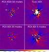 |
Fig. 6. IFS example: final images using PCA/ASDI (50 modes), PCA/ADI (20 and 5 modes), and TLoci. Images are corrected from the technique throughput and from the coronagraph transmission. The color scale. which is the same for all images, shows the contrast to the star ratio. The spatial scale is the same for all images. |
5.2. Measurements of photometry
For TLoci and PCA/ADI 5 mode images, we use the model of planet image technique (Sect. 3.2) to extract the photometry and the astrometry of the three fake planets. For the PCA/ADI 20 mode image, we use the negative planet technique (Sect. 3.3) to avoid the photometry underestimation that was noticed in Sect. 4.2. When considering the spectral channels where the planet is detected, the astrometry measurements are accurate with 1 σ uncertainties of 0.6, 0.3, and 0.5 pixel for planets 1, 2, and 3 respectively. These values correspond to 4.5, 2.3, and 3.8 mas respectively.
We plot the extracted spectrophotometry in Figs. 7–9 for the TLoci/ADI (blue), the PCA/ADI 5 modes (red), and the PCA/ADI 20 modes (green) cases, as well as the true spectra that we used for the fake planets (full line). The arrows give the 1 σ upper limits when the planet is not detected, and the error bars correspond to the estimated 1 σ uncertainties.
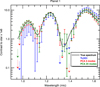 |
Fig. 7. Spectra of planet-to-star contrast extracted from the PCA/ADI 5 modes (red), PCA/ADI 20 modes (green), and TLoci/ADI (blue) images compared to the true spectrum that was used for fake planet 1 (black full line). Error bars and upper limits are given at 1 σ. |
All algorithms retrieve the spectra of the three fake planets with similar uncertainties and no bias. In the case of planet 3, which is in a region with bright speckles, there are spectral channels below 1 μm for which TLoci give an upper limit only (no detection). For the same planet, the PCA algorithm using 5-modes does not detect the object between 1.3 µm and 1.5 µm, whereas it does below 1 µm. Such a situation often happens: several algorithms detect the planet in different spectral channels. Thus, it is essential to use several algorithms in parallel to optimize the detection and the measured spectrum.
6. Conclusion
The Speckle Calibration tool (SpeCal) was developed by the SPHERE/VLT consortium in the context of a large survey (SHINE), the main objective of which is to search for and measure the astrometry and spectrophotometry of exoplanets at large separations (>5 au). SpeCal provides high contrast images using a variety of algorithms (cADI, PCA, Loci, TLoci) enabling the study of exoplanets, brown dwarfs, and circum-stellar disks. SpeCal has been intensively tested on SPHERE guaranteed time observations (GTO) and calibration data since 2013. It is implemented in the SPHERE data center (Delorme et al. 2017a) to produce the final reduction for public data releases. The final reductions will be available in the SPHERE target database (TDB1). Finally, SpeCal and the DC are able to process all GTO data obtained with IRDIS/SPHERE (dual-band imaging) and IFS/SPHERE (integral field spectrometer) automatically.
SpeCal delivers major outputs for the survey and feeds the SPHERE database with final images, contrast curves, S/N maps, astrometry, and photometry of detected point-like sources in the field (exoplanets, brown dwarfs, background sources, and all sub-stellar or stellar candidates). This material has been used for the study of exoplanets and circumstellar disks primarily based on SPHERE data (de Boer et al. 2016; Ginski et al. 2016; Lagrange et al. 2016; Maire et al. 2016a, 2017; Mesa et al. 2016, 2017; Perrot et al. 2016; Vigan et al. 2016; Zurlo et al. 2016; Benisty et al. 2017; Bonavita et al. 2017; Bonnefoy et al. 2017; Feldt et al. 2017; Pohl et al. 2017; Samland et al. 2017).
In this paper, we investigated the astrometric and photometric performance for point-like sources considering objects at a contrast of ~3 × 10⁻⁶ in the separation range of 3–26 FWHM. Using the techniques of positive and negative fake planets, we demonstrated the ability to achieve a measurement of the astrometry with an accuracy of ~0.2 pixel (i.e., ~2 mas) for IRDIS and 0.5 pixel (i.e., ~4 mas) for IFS. Similarly the photometric accuracy reaches ~10%.
We are planning to upgrade SpeCal with other algorithms like Andromeda (Cantalloube et al. 2015) or inverse approaches (Devaney & Thiébaut 2017), and other observing modes (polarimetry, ZIMPOL). Finally, a specific tool to model the ADI self-subtraction of circumstellar disks with simple geometries will also be implemented.
Acknowledgments
SPHERE is an instrument designed and built by a consortium consisting of IPAG (Grenoble, France), MPIA (Heidelberg, Germany), LAM (Marseille, France), LESIA (Paris, France), Laboratoire Lagrange (Nice, France), INAF – Osservatorio di Padova (Italy), Observatoire astronomique de l’Université de Genève (Switzerland), ETH Zurich (Switzerland), NOVA (Netherlands), ONERA (France), and ASTRON (Netherlands), in collaboration with ESO. SPHERE was funded by ESO, with additional contributions from the CNRS (France), MPIA (Germany), INAF (Italy), FINES (Switzerland), and NOVA (Netherlands). SPHERE also received funding from the European Commission Sixth and Seventh Framework Programs as part of the Optical Infrared Coordination Network for Astronomy (OPTICON) under grant number RII3-Ct-2004-001566 for FP6 (2004–2008), grant number 226604 for FP7 (2009–2012), and grant number 312430 for FP7 (2013–2016). This work has made use of the SPHERE data center, jointly operated by Osug/Ipag (Grenoble), Pytheas/Lam/Cesam (Marseille), OCA/Lagrange (Nice), and Observatoire de Paris/Lesia (Paris) and supported by a grant from Labex OSUG@2020 (Investissements d’avenir – ANR10 LABX56). We acknowledge financial support from the French ANR GIPSE, ANR-14-CE33-0018. Dino Mesa acknowledges support from the ESO-Government of Chile Joint Committee program “Direct imaging and characterization of exoplanets”.
References
- Amara, A., & Quanz, S. P. 2012, MNRAS, 427, 948 [NASA ADS] [CrossRef] [Google Scholar]
- Baba, N., & Murakami, N. 2003, PASP, 115, 1363 [NASA ADS] [CrossRef] [Google Scholar]
- Baba, N., Murakami, N., Tate, Y., Sato, Y., & Tamura, M. 2005, Proc. SPIE, 5905, 347 [Google Scholar]
- Benisty, M., Stolker, T., Pohl, A., et al. 2017, A&A, 597, A42 [NASA ADS] [CrossRef] [EDP Sciences] [Google Scholar]
- Beuzit, J.-L., Mouillet, D., Lagrange, A.-M., & Paufique, J. 1997, A&AS, 125, 175 [NASA ADS] [CrossRef] [EDP Sciences] [Google Scholar]
- Beuzit, J.-L., Feldt, M., Dohlen, K., et al. 2008, Proc. SPIE, 7014, 701418 [Google Scholar]
- Boccaletti, A., Thalmann, C., Lagrange, A.-M., et al. 2015, Nature, 526, 230 [NASA ADS] [CrossRef] [Google Scholar]
- Bonavita, M., D’Orazi, V., Mesa, D., et al. 2017, A&A, 608, A106 [NASA ADS] [CrossRef] [EDP Sciences] [Google Scholar]
- Bonnefoy, M., Milli, J., Ménard, F., et al. 2017, A&A, 597, L7 [NASA ADS] [CrossRef] [EDP Sciences] [Google Scholar]
- Cantalloube, F., Mouillet, D., Mugnier, L. M., et al. 2015, A&A, 582, A89 [NASA ADS] [CrossRef] [EDP Sciences] [Google Scholar]
- Chauvin, G., Lagrange, A.-M., Beust, H., et al. 2012, A&A, 542, A41 [NASA ADS] [CrossRef] [EDP Sciences] [Google Scholar]
- Chauvin, G., Desidera, S., Lagrange, A.-M., et al. 2017, A&A, 605, L9 [CrossRef] [EDP Sciences] [Google Scholar]
- Claudi, R. U., Turatto, M., Gratton, R. G., et al. 2008, Proc. SPIE, 7014, 70143E [Google Scholar]
- de Boer, J., Salter, G., Benisty, M., et al. 2016, A&A, 595, A114 [NASA ADS] [CrossRef] [EDP Sciences] [Google Scholar]
- Delorme, P., Meunier, N., Albert, D., et al. 2017a, SF2A Proc. of the Annual meeting of the French Society of Astronomy and Astrophysics, 347 [Google Scholar]
- Delorme, P., Schmidt, T., Bonnefoy, M., et al. 2017b, A&A, 608, A79 [NASA ADS] [CrossRef] [EDP Sciences] [Google Scholar]
- Devaney, N., & Thiébaut, É. 2017, MNRAS, 472, 3734 [NASA ADS] [CrossRef] [Google Scholar]
- Dohlen, K., Langlois, M., Saisse, M., et al. 2008, Proc. SPIE, 7014, 70143L [Google Scholar]
- Feldt, M., Olofsson, J., Boccaletti, A., et al. 2017, A&A, 601, A7 [NASA ADS] [CrossRef] [EDP Sciences] [Google Scholar]
- Galicher, R., & Marois, C. 2011, 2nd Int. Conf. on Adaptive Optics for Extremely Large Telescopes, P25 http://ao4elt2.lesia.obspm.fr [Google Scholar]
- Ginski, C., Stolker, T., Pinilla, P., et al. 2016, A&A, 595, A112 [NASA ADS] [CrossRef] [EDP Sciences] [Google Scholar]
- Guerri, G., Daban, J.-B., Robbe-Dubois, S., et al. 2011, Exp. Astron., 30, 59 [NASA ADS] [CrossRef] [Google Scholar]
- Lafrenière, D., Marois, C., Doyon, R., Nadeau, D., & Artigau, É. 2007, ApJ, 660, 770 [NASA ADS] [CrossRef] [Google Scholar]
- Lagrange, A.-M., Bonnefoy, M., Chauvin, G., et al. 2010, Science, 329, 57 [NASA ADS] [CrossRef] [PubMed] [Google Scholar]
- Lagrange, A.-M., Langlois, M., Gratton, R., et al. 2016, A&A, 586, L8 [NASA ADS] [CrossRef] [EDP Sciences] [Google Scholar]
- Lawson, C., & Hanson, R. 1995, Solving Least Squares Problems (Philadelphia: Society for Industrial and Applied Mathematics) [Google Scholar]
- Maire, A.-L., Boccaletti, A., Rameau, J., et al. 2014, A&A, 566, A126 [NASA ADS] [CrossRef] [EDP Sciences] [Google Scholar]
- Maire, A.-L., Bonnefoy, M., Ginski, C., et al. 2016a, A&A, 587, A56 [NASA ADS] [CrossRef] [EDP Sciences] [Google Scholar]
- Maire, A.-L., Langlois, M., Dohlen, K., et al. 2016b, Proc. SPIE, 9908, 990834 [CrossRef] [Google Scholar]
- Maire, A.-L., Stolker, T., Messina, S., et al. 2017, A&A, 601, A134 [NASA ADS] [CrossRef] [EDP Sciences] [Google Scholar]
- Marois, C., Racine, R., Doyon, R., Lafrenière, D., & Nadeau, D. 2004, ApJ, 615, L61 [NASA ADS] [CrossRef] [Google Scholar]
- Marois, C., Lafrenière, D., Doyon, R., Macintosh, B., & Nadeau, D. 2006, ApJ, 641, 556 [Google Scholar]
- Marois, C., Macintosh, B., & Véran, J. 2010, Proc. SPIE, 7736, 77361J [CrossRef] [Google Scholar]
- Marois, C., Correia, C., Véran, J.-P., & Currie, T. 2014, IAU Symp., 299, 48 [Google Scholar]
- Mawet, D., Milli, J., Wahhaj, Z., et al. 2014, ApJ, 792, 97 [NASA ADS] [CrossRef] [Google Scholar]
- Mesa, D., Gratton, R., Zurlo, A., et al. 2015, A&A, 576, A121 [NASA ADS] [CrossRef] [EDP Sciences] [Google Scholar]
- Mesa, D., Vigan, A., D’Orazi, V., et al. 2016, A&A, 593, A119 [NASA ADS] [CrossRef] [EDP Sciences] [Google Scholar]
- Mesa, D., Zurlo, A., Milli, J., et al. 2017, MNRAS, 466, L118 [NASA ADS] [CrossRef] [Google Scholar]
- Milli, J., Hibon, P., Christiaens, V., et al. 2017, A&A, 597, L2 [NASA ADS] [CrossRef] [EDP Sciences] [Google Scholar]
- Pavlov, A., Möller-Nilsson, O., Feldt, M., et al. 2008, Proc. SPIE, 7019, 701939 [CrossRef] [Google Scholar]
- Perrot, C., Boccaletti, A., Pantin, E., et al. 2016, A&A, 590, L7 [NASA ADS] [CrossRef] [EDP Sciences] [Google Scholar]
- Pohl, A., Sissa, E., Langlois, M., et al. 2017, A&A, 605, A34 [NASA ADS] [CrossRef] [EDP Sciences] [Google Scholar]
- Racine, R., Walker, G. A. H., Nadeau, D., Doyon, R., & Marois, C. 1999, PASP, 111, 587 [NASA ADS] [CrossRef] [Google Scholar]
- Rameau, J., Chauvin, G., Lagrange, A.-M., et al. 2015, A&A, 581, A80 [NASA ADS] [EDP Sciences] [Google Scholar]
- Rosenthal, E. D., Gurwell, M. A., & Ho, P. T. P. 1996, Nature, 384, 243 [NASA ADS] [CrossRef] [Google Scholar]
- Samland, M., Mollière, P., Bonnefoy, M., et al. 2017, A&A, 603, A57 [NASA ADS] [CrossRef] [EDP Sciences] [Google Scholar]
- Soummer, R., Pueyo, L., & Larkin, J. 2012, ApJ, 755, L28 [NASA ADS] [CrossRef] [Google Scholar]
- Thalmann, C., Schmid, H. M., Boccaletti, A., et al. 2008, Proc. SPIE, 7014, 70143F [Google Scholar]
- Thatte, N., Abuter, R., Tecza, M., et al. 2007, MNRAS, 378, 1229 [NASA ADS] [CrossRef] [Google Scholar]
- Vigan, A., Moutou, C., Langlois, M., et al. 2010, MNRAS, 407, 71 [NASA ADS] [CrossRef] [Google Scholar]
- Vigan, A., Bonnefoy, M., Ginski, C., et al. 2016, A&A, 587, A55 [NASA ADS] [CrossRef] [EDP Sciences] [Google Scholar]
- Zurlo, A., Vigan, A., Mesa, D., et al. 2014, A&A, 572, A85 [NASA ADS] [CrossRef] [EDP Sciences] [Google Scholar]
- Zurlo, A., Vigan, A., Galicher, R., et al. 2016, A&A, 587, A57 [NASA ADS] [CrossRef] [EDP Sciences] [Google Scholar]
All Tables
Acronyms and names of algorithms used to process the data recorded using a given strategy of observation (third column).
Separations to the central star in pixels towards east (ΔRA) and north (ΔDec), angular separations in mas and flux ratio with respect to the star (C) for each fake planet added to the IRDIS data.
Fake planets injected in the IFS data: separation from the central star in pixels toward east (ΔRA) and toward north (ΔDec), angular separation in mas, and averaged contrast over the 39 spectral channels.
All Figures
|
Fig. 1. Loci and TLoci regions of interest (left figure and central blue region in the right figure) and TLoci optimizing region (exterior red region in the right figure). |
| In the text | |
|
Fig. 2. Real (left) and estimated (right) images of an off-axis source in an ADI reduced image showing the negative wings due to self-subtraction of the planet flux. |
| In the text | |
|
Fig. 3. IRDIS example: final images using cADI, Tloci, Loci, PCA (5 and 10 modes). Images are corrected from the technique throughput and from the coronagraph transmission. The color scale, which is the same for all images, shows the contrast to the star ratio. The spatial scale is the same for all images. |
| In the text | |
|
Fig. 4. Contrast curves at 5 σ before (ClasImg) and after minimization of the stellar light using different algorithms (cADI, Tloci, Loci, PCA 5 modes) on H2 data. The curves are corrected from the technique attenuation and from the coronagraph transmission. The fake planets are represented by plus symbols. |
| In the text | |
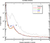 |
Fig. 5. Same as Fig. 4 for H3-band. |
| In the text | |
|
Fig. 6. IFS example: final images using PCA/ASDI (50 modes), PCA/ADI (20 and 5 modes), and TLoci. Images are corrected from the technique throughput and from the coronagraph transmission. The color scale. which is the same for all images, shows the contrast to the star ratio. The spatial scale is the same for all images. |
| In the text | |
|
Fig. 7. Spectra of planet-to-star contrast extracted from the PCA/ADI 5 modes (red), PCA/ADI 20 modes (green), and TLoci/ADI (blue) images compared to the true spectrum that was used for fake planet 1 (black full line). Error bars and upper limits are given at 1 σ. |
| In the text | |
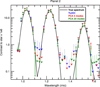 |
Fig. 8. Same as Fig. 7 for the fake planet 2. |
| In the text | |
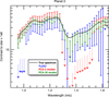 |
Fig. 9. Same as Fig. 7 for the fake planet 3. |
| In the text | |
Current usage metrics show cumulative count of Article Views (full-text article views including HTML views, PDF and ePub downloads, according to the available data) and Abstracts Views on Vision4Press platform.
Data correspond to usage on the plateform after 2015. The current usage metrics is available 48-96 hours after online publication and is updated daily on week days.
Initial download of the metrics may take a while.