| Issue |
A&A
Volume 615, July 2018
|
|
|---|---|---|
| Article Number | A143 | |
| Number of page(s) | 10 | |
| Section | Planets and planetary systems | |
| DOI | https://doi.org/10.1051/0004-6361/201732474 | |
| Published online | 06 August 2018 | |
Oscillations of cometary tails: a vortex shedding phenomenon?★
1
Centre for Fusion, Space and Astrophysics, University of Warwick,
Coventry, CV4 7AL,
UK
e-mail: This email address is being protected from spambots. You need JavaScript enabled to view it.
2
Institut für Astrophysik, Georg-August-Universität,
Göttingen, 37077,
Germany
3
Naval Research Laboratory,
Washington, DC 20375,
USA
Received:
15
December
2017
Accepted:
29
March
2018
Abstract
Context. During their journey to perihelion, comets may appear in the field of view of space-borne optical instruments, showing in some cases a nicely developed plasma tail extending from their coma and exhibiting an oscillatory behaviour.
Aims. The oscillations of cometary tails may be explained in terms of vortex shedding because of the interaction of the comet with the solar wind streams. Therefore, it is possible to exploit these oscillations in order to infer the value of the Strouhal number S t, which quantifies the vortex shedding phenomenon, and the physical properties of the local medium.
Methods. We used the Heliospheric Imager (HI) data of the Solar TErrestrial Relations Observatory (STEREO) mission to study the oscillations of the tails of comets 2P/Encke and C/2012 S1 (ISON) during their perihelion in Nov 2013. We determined the corresponding Strouhal numbers from the estimates of the halo size, the relative speed of the solar wind flow, and the period of the oscillations.
Results. We found that the estimated Strouhal numbers are very small, and the typical value of S t ~ 0.2 would be extrapolated for size of the halo larger than ~106 km.
Conclusions. Although the vortex shedding phenomenon has not been unambiguously revealed, the findings suggest that some kind of magnetohydrodynamic (MHD) instability process is responsible for the observed behaviour of cometary tails, which can be exploited for probing the physical conditions of the near-Sun region.
Key words: solar wind / comets: individual: Encke, ISON / magnetohydrodynamics (MHD) / methods: observational / instabilities / waves
The movies associated to Figs. 1 and 4 are available at http://www.aanda.org
© ESO 2018
1 Introduction
Optical instruments aboard space missions, like the Solar Heliospheric Observatory (SoHO)/LASCO (Brueckner et al. 1995) and the Solar TErrestrial RElations Observatory (STEREO)/SECCHI coronagraphs (Kaiser 2005) have returned observations of more than 3200 new and previously known comets (Battams & Knight 2017). More than 85% of these have a perihelion very close to the Sun, and are defined as “sungrazing” comets. Usually, they disappear before reaching their perihelion, as a result of fragmentation and vaporisation at distances of typically between six and ten solar radii (Biesecker et al. 2002; Knight et al. 2012). However, a few exceptional cases of comets flying inside the solar corona and observed by extreme ultra-violet (EUV) imagers (Schrijver et al. 2012; Downs et al. 2013; McCauley et al. 2013) have been reported.
One area of interest in comets is related to the possibility of exploiting them as natural probes of the solar corona and near-Sun environment (Ramanjooloo 2015). A tail of ions from the cometary nuclei is formed, which interacts with the local medium exhibiting a swaying-like motion, as is also evident with the first observation of comet 2P/Encke in 2007 with the Heliospheric Imager (HI) 1 of STEREO-A (Vourlidas et al. 2007). The features observed in Encke’s tail have been interpreted in terms of turbulent eddies rooted in the solar wind and traced by the cometary plasma (DeForest et al. 2015). On the other hand, the observed comet-solar wind system is more analogous to that of an object of finite size immersed in a flow with a Kármán vortex street formed in the wake of the obstacle.
The phenomenon of vortex shedding has been widely invoked both in science and engineering. In solar physics it has been used to explain the excitation and selectivity of kink oscillations in coronal loops (Nakariakov et al. 2009) and global oscillations of halo coronal mass ejections (CMEs) measured with coronagraphs (Lee et al. 2015). Moreover, vortices due to Kelvin-Helmholtz (KH) instability have been observed at the flanks of an expanding CME (Foullon et al. 2011). In the context of comets, the interaction of the solar wind with the cometary halo may lead to the formation of shed vortices: the ion tail would periodically oscillate as a consequence of the appearance of a periodic force caused by the succession of eddies with opposite vorticity, similar to flags waving in a wind. The fluid behaviour past an obstacle is described by the well-known Reynolds number Re = V L∕ν (with V the relative flow speed, L the obstacle size, and ν the kinematic viscosity), and the Strouhal number S t = L∕(PV), which takes into account the period P of the shed vortices. The relationship between them is not unambiguously established (Sakamoto & Haniu 1990; Ponta & Aref 2004), but it can be used for the estimation of the kinematic viscosity of the fluid. Here, we aim to analyse the dynamics of the tails of 2P/Encke and the sungrazing comet C/2012 S1 (ISON) observed with the HI-1 and 2 of STEREO-A during their perihelion in 2013 in the context of the vortex shedding phenomenon. The paper is organised as follows. In Sect. 2 we present the overall observations. Values of the S t numbers (and the associated Re ones) from the estimates of the halo size, the relative speed of the solar wind flow, and the properties of the observed oscillations (wavelength, period, amplitude) of the tails are shown in Sect. 3. The discussion and conclusions are presented in Sect. 4. We demonstrate how these observations can be exploited to determine the physical properties of the solar wind plasma.
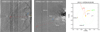 |
Fig. 1 Running difference images of Encke and ISON from STEREO-A/HI-2 (left panel) and HI-1 (middle panel). Orbits of comets Encke (yellow line) and ISON (red line) in the Heliocentric-Aries-Ecliptic (HAE) coordinate system (right panel). Dashed lines indicate where the trajectory is below the ecliptic plane. The Earth is represented by the green dot (with the associated orbit dashed line style), while STEREO-A and B are shown with the red and blue dots, respectively. For reference, the position of the inner planets is also shown. The corresponding animations for each panel are available online. |
2 Observations and data
The HI-1 telescope of STEREO A provides white-light images of the inner heliosphere covering a field-of-view between ~4° and ~24° of solar elongation angles from the east solar limb (~15 − 84 R⊙), with a pixel size of 1.2 arcmin (~72 arcsec) (Howard et al. 2008), while HI-2 observes the outer heliosphere with an angular range of ~ 19°−~89° (66− 318 R⊙), with an image pixel size of 4.3 arcmin. The typical cadence of each instrument is 40 and 120 min, respectively, with exposure time of typically 40-minute. We used Level 2 FITS files from the UK Solar System Data Centre1, based on one-day background subtracted for HI-1, and three-day background subtracted for HI-2 to remove the excess of the F-corona brightness and stray light, and covering a time interval between 5 Nov and 9 Dec 2013. We read the FITS files using the routine mreadfits, which is part of SolarSoftWare (SSW)2, and obtained the corresponding headers and image arrays with size of 1024 × 1024 pixels.
To better reveal the fluctuations of the tails, HI images have been processed for background stars removal by cross-correlating each pair of consecutive images from our dataset: we found the relative pixel shift between them, translated the subtrahend image of this amount, and finally performed the difference. An example of the images is given in Fig. 1. The positions of Encke and ISON during the entire time of the observations were found by de-projecting the ephemerides of the comets to the STEREO-A/HI images using the routines fitshead2wcs and wcs_get_pixel of the World Coordinate Systems (WCS) package, which is included in SSW (Thompson & Wei 2010). The ephemerides were initially read and processed with the SPICE3 software, which is part of the Navigation and Ancillary Information Facility (NAIF) and also implemented in SSW with the SUNSPICE package. SPICE kernels of the comets (i.e. files in .bsp format storing the ephemerides) were downloaded4, and loaded by the cspice_furnsh routine. Position and velocity in a desired coordinate system were obtained with get_sunspice_coord, and then used to make the plots in the right-hand panel of Figs. 1 and 2. Then, we created a series of running difference sub-images with a new reference frame co-moving with each single comet (Fig. 1). In these images the comet’s head is fixed, while the tail almost lies along the horizontal axis. The orbital properties of Encke and ISON are different (Fig. 1, right panel, and Fig. 2): Encke reached the perihelion at 0.33 AU on 21 Nov 2013 with an orbital speed of ~70 km s−1, and at the time of the observations its orbit was pretty close to the solar equatorial plane (between approximately –10° and +10° in latitude).Conversely, ISON orbited along a hyperbolic trajectory, spanning several degrees in latitude at the perihelion with the closest distance at 0.01 AU from the Sun’s centre (just ~ 1.15 R⊙ from the solar photosphere) reached on 28 Nov 2013, with an orbital velocity of almost 400 km s−1. However, when observed with HI-1 (until approximately 26 Nov), both comets had similar orbital speeds and latitudes, moving out of the plane of observations of the instrument (located at ~ 0.95 AU, dashed-blue line in the bottom left panel of Fig. 2): the distance of ISON from STEREO A ranged between ~ 1.15 − 0.95 AU, while that of Encke between ~1.2 − 0.6 AU during the time of the observations.
3 Analysis
To quantity the Strouhal number, we must estimate typical values of the size of the cometary halo L, which plays the role of an obstacle immersed in the solar wind flow, the relative speed comet-solar wind V, and the period P of the tail oscillation, which we assume equivalent to that of the hypothetical shed vortices.
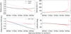 |
Fig. 2 Left panels: variation of the distance from the Sun (top panel) for Encke (black) and ISON (red), and from STEREO-A in AU (bottom panel). Continuous lines mark the time intervals when the comets are visible in the HI-1 FoV, dotted lines the opposite. The blue dashed line in the bottom panel indicates the STEREO A-Sun distance, which is a reference line to visualise when the comets are behind or in front of the plane-of-sky. Right panels: orbital speed of the comets (top panel), and variation of the latitude in the Helio-Centric-Inertial (HCI) coordinate system (bottom panel). |
3.1 Determination of the halo size
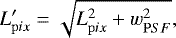
The size of the halos was inferred by constructing time-distance (TD) maps from the normal intensity images with a vertical slit across the comet’s head (Fig. 3) in the processed HI-1 sub-images. The horizontal bright feature at the centre of the TD maps is the signature of the comet’s halo. We determined the size by fitting the intensity profile with a Gaussian function at each time (we used the MPFIT routines by Markwardt 2009). The intensity profile across the halo is sampled over 11 pixels across: 4 pixels at the sides of this spatial interval are taken as a background (shaded region in the middle panels of Fig. 3), which is fitted with a linear function added to the Gaussian function (red). The full-width of the Gaussian function at the background intensity level is chosen as a good approximation for the apparent size of the halo  , where Im ax (t) is the height of the peak intensity of the coma, and Iback the average value of the background intensity of ~0.1 DN s−1. Measurements are strongly affected by the point-spread function (PSF) of HI-1A, which is estimated to be of the order of wPSF = 1.48−1.69 pixel (Bewsher et al. 2010). In addition, the limiting magnitude for HI-1 is approximately 13.5. In a way similar to what is shown by Aschwanden et al. (2008) for coronal loops, the effective size of the coma measured in pixel units
  is given by
 (1)
(1)
which is used to determine Lpix. These values are converted into physical units by considering the radius of the Sun in arcsec (retrieved from the header under the keyword RSUN), and the image plate scale Δpix ≈ 0.02 deg pix−1 ≈ 0.5 × 10⁵ km pix−1 (CDELT1 keyword), both defined at the STEREO A-Sun distance (dS un, obtained from the header keyword DSUN_OBS) and corrected for the relative distance dC comet-observer (calculated via get_sunspice_lonlat). Therefore, the size of the halo is found as L = Lpix Δpix dC∕dSun. The data points for both comets are fitted with a linear function (red line in the bottom panels of Fig. 3): ISON presents a clear increase of the halo size over time, while the Encke’s halo size is slightly decreasing (we did not consider the broader cloud of data points since these values are affected by the low contrast between the Encke’s brightness and the background). Average values of the halo size are found to be LE ncke = (1.54 ± 0.16) × 105 km, and LI SON = (1.79 ± 0.22) × 105 km. These estimates are consistent with typical values of cometary halos and comas found in literature, which can also reach values of 106 − 107 km (Ramanjooloo 2015).
3.2 Determination of the relative speed
Values of the relative speed of the solar wind past the halos strongly depend on the comet orbits and the intrinsically variable nature of the solar wind speed, which ranges between 300 (slow wind) and 800 km s−1 (fast wind). Accurate knowledge of the solar wind speed at the positions of the comets would require forward modelling or extrapolations based upon the conditions of the solar corona and/or satellite measurements. The top left panel of Fig. 4 shows the solar wind speed on the solar equatorial plane provided by the ENLIL model (Odstrcil 2003) at the time of Encke’s perihelion in the Helio-Earth-EQuatorial (HEEQ) coordinate system. Both comets seem to cross different solar wind streams that have speeds between 300–450 km s−1. The relative speed V is determined by the vectorial sum of the solar wind flow VSW and the orbital comet speed VC, that is V = VSW −VC, and the plasma tail should extend along this resulting vector, which forms an angle with the solar wind direction defined as the aberration angle (Fig. 4-top-right).
The aberration angle α between the relative speed vector and the radial direction is defined as 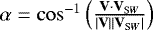 . Therefore, given VC, we determined the function α = α(t, VSW) in the time range of the observationsand for different values of VSW (200, 400, 600, ... km s−1), and visually compared the hypothetical aberration angle profiles (de-projected according to the STEREO A view) with the location of the tail inferred from a TD map. The TD maps in Fig. 4 show the normal intensity extracted from a semi-circular slit located at 20 and 60 pixels from the coma centre of Encke and ISON, respectively. The 0 in the vertical axis coincides with the projected radial direction comet-Sun. The aberration angle profiles are overplotted for different values of the radial solar wind speed VSW. When both comets are relatively far from their perihelion, the different aberration profiles tend to coincide because of projection effects (the tails extend along the apparent radial direction). Close to perihelion, the tails undergo a considerable angular deviation, which is well-fitted by a solar wind speed of 400 km s−1 in the case of Encke. The same is not unambiguously clear for ISON, and the position of the tail may be affected by other factors, such as the hyperbolic orbit of the comet, spurious projection effects, the nature of the solar wind out of the equatorial plane, or the composition of ISON’s tail (e.g. strong percentage of dust particles) which would affect the direction. Despite this, we have considered an average solar wind flow VS W= 400 km s−1 even for ISON. Itis interesting to notice that periodic changes in the solar wind speed can determine periodic variation of the aberration angle, hence oscillations of the cometary tails (see the green line in the middle left panel of Fig. 4). The green oscillatory pattern in Encke’s TD map is obtained with an amplitude velocity of 50 km s−1 (of the order of the Alfvén speed in the solar wind). However, the oscillations are not evident when the projected aberration and radial direction coincide. In addition, other parameters such as solar wind density or the magnetic field vector could somehow influence the observed oscillations, but we have not considered any quantified contribution in the present study.
After having defined the most probable solar wind speed (in our case 400 km s−1), the magnitude of the relative flow is found as  . The bottom right panel of Fig. 4 shows the profile of the relative speed V for Encke and ISON during the observations: the relative speed for Encke is limited between approximately 380 and 440 km s−1, while for ISON it reaches values up to ~650 km s−1 at the perihelion.
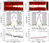 |
Fig. 3 Time-distance maps (top panels), example of intensity profiles with related fittings (middle panels), and L vs. time (bottom panels) for Encke and ISON’s halo with HI-1A. |
3.3 Determination of the period
Periods for the oscillations of the tail were determined by TD maps constructed with a vertical slit located at a given distance (e.g. 40, 50, 60, ... pixels) from the comet’s coma in the processed running difference sub-images. An example is given in Fig. 5, where the TD maps for comets Encke and ISON in HI-1A are extracted from a slit located at 50 pixels (1.0 deg ≈ 2.5 × 10⁶ km) from the comet’s coma. The manually-determined points were fitted with a sinusoidal function plus a linear function to take into account any possible deviation from the local zero
 (2)
(2)
In order to detect different possible regime of oscillations, we divided the obtained times series in consecutive intervals of 10, 20, 30, 60, and 90 h. Periods ranging between 5 and 20 h have been measured both for Encke and ISON. We considered only those periods having a relative error σP∕P < 30% obtained from fittingswith χ2 < 10 to be good estimates. The amplitude of the fitted oscillations was also scaled by the factor dC ∕dSun in order to account for the distance comet-observer.
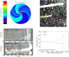 |
Fig. 4 Top left panel: solar wind speed on the solar equatorial plane provided by ENLIL. Earth’s position is fixed and represented by a green dot, while STEREO A and B are shown with red and blue dots, respectively. The trajectories of Encke and ISON projected on this plane are shown in orange and red, respectively, with some dots showing the positions of the comets with an interval of four days between 10 Nov and 4 Dec. The corresponding movie is available online. Top right panel: projected radial direction from the Sun, the projected direction of the orbital speed for Encke (red), and the resulting vectors V (yellow) determined as a vectorial sum between the solar wind VSW and the comet speed VC vectors. For a solar wind speed of 400 km s−1, the projected direction of V almost coincides with the tail direction. Bottom left panels: time-distance maps for Encke and ISON showing the inclination of the tail (the bright feature) with respect to the projected radial direction, and compared for different profiles of the aberration angle. In one case, we show the behaviour of the aberration angle profile for Encke assuming a sinusoidally variable solar wind with mean value of 400 km s−1, amplitude of 50 km s−1, and period of 12 h. Bottom right panel: plot of the relative speed magnitude V vs. time of observations assuming a constant and radial solar wind speed of 400 km s−1. |
3.4 Estimation of the Strouhal numbers
By relating the estimated frequencies f = 1∕P and the corresponding relative speeds V, we fitted the data points with a linear function f = kV, where k = St∕L (Fig. 6, top left panel). We have not considered a time lag between the value of V and f, since some delay is reasonably expected between the times when the halo encounters a given speed, the vortex is formed, advected with a given phase speed and then measured at a given distance from the halo. Hence, the data points should be moved towards lower speeds, but this would be a minor correction. Given k and L, we find Strouhal numbers of the order of 10−3, which are considerably small, with some values between 0.02–0.1 (Fig. 6). In hydrodynamics S t ≈ 0.2 for a very broad range of parameters, which should be associated with f−1 ≈ 0.3 h for L= 105, and V = 400 km s−1. By extrapolating S t at higher values of L using the determined coefficientsk, we find that values of S t ≈ 0.15 − 0.4 are obtained for L ≈ 2.5−7.2 × 10⁶ km (Fig. 6, top right panel), which are very large, even if in agreement with typical scale lengths. For example, Ulysses crossed the tail of comet Hyakutake in 1996 at a distance of 3.8 AU from its nucleus, and measured a diameter of ~ 7 ×10⁶ km (Jones et al. 2000). However, such a value is improbable in the proximity of a nucleus (indeed the tail undergoes cross-sectional expansion), and an upper limit value can be reasonably considered as 1 × 10⁶ km (assuming that the outermost layers are indeed not detected with HI-1), which should represent the size of the overall draped magnetic structure around the cometary nucleus. On the other hand, a halo of hydrogen is developed around comets with a diameter even larger than the Sun. The parameter L can be associated with the size of the shed vortices, which undergo expansion due to diffusivity. Our oscillations are measured at prescribed distances from the coma, where the oscillation amplitudes in a few cases have values of the order of 106 km, which, however, markedly deviate from the sample distribution (Fig. 7).
In the middle and bottom panels of Fig. 6, we plot the values of S t for each data point (we used the local oscillation amplitude as L), showing how it changes with time, the local oscillation amplitude, the frequency f, and the relative speed V. Some extreme values are larger than 0.02, corresponding to the extreme amplitude values mentioned previously, but in general the cloud of points lies under S t ≈ 0.01.
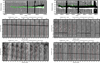 |
Fig. 5 Top panels: time-distance maps for Encke and ISON in HI-1A and HI-2A with showing the manually determined data points tracking the oscillations. Middle and bottom panels: sequences of 10 consecutive frames for Encke and ISON with some sinusoids indicating propagating waves along the tail. Values of amplitude, wavelength, and phase of the oscillations are reported on each single frame. The time-steps in min from the first frame of the sequence are shown on the top horizontal axis for each frame. |
4 Discussion and conclusions
The small values of the estimated Strouhal number raise the questions of whether the observed kink-like oscillations of the plasma tail are induced by the solar wind variability (e.g. due to CMEs), or associated with vortex shedding-like phenomena. In the former case, the observed oscillations would be not natural, and it would require the oscillation in the wind to be, as we observed in the tail, monochromatic and of a large amplitude. In addition, for the excitation of the oscillations of the kink symmetry in the tail, the oscillation in the wind should be of the same kink symmetry and we are not aware of this. Thus, we should disregard this interpretation on this basis. Another option is that the oscillations in the solar wind excite natural modes of the tail by resonance. In this case the oscillations in the wind could be broad-band, and only the resonating harmonics take part in the excitation of the natural modes in the tail (i.e. a harmonic oscillator driven by a broad-band force). However, in this scenario the tail oscillation, should grow gradually, and also, variations of the phase of the induced oscillation in the tail would be expected, which we do not see either.
In the latter case, the tail oscillations may be associated with a breakdown of the proper Kármán vortex street into a secondary structure (Johnson 2004; Dynnikova et al. 2016). Something similar also appears in the simulations of Gruszecki et al. (2010; see their Fig. 1), where the entire vortex street has an oscillatory structure, with a wavelength four to five times larger than the vortex size (presumably the period should be four to five times longerthan the vortex shedding period, if we assume identical phase speed in both regimes). In such a case, our estimates for S t should be corrected by the same factors, hence S t values will range between ≈0.02 and 0.3. On the other hand, small-scale perturbations appear in the tails of Encke and ISON (white arrows in Fig. 8), which, however, have not been properly considered in the present study because of limitations in the spatial resolution of the instruments and intensity contrast.
It is interesting to notice that the comet tail-solar wind flow can be modelled in terms of a damped driven harmonic oscillator:
 (3)
(3)
with y being the displacement, ω0 the natural frequency of the magneto-acoustic mode of the tail (which can be assimilated to a plasma cylinder), F(t) the amplitude of the external force, ωs h (t) = 2πStV (t)∕(nL) the vortex shedding pulsation (we added an artificial factor n to model the possible contribution from a low-frequency mode for n > 1, n = 1 would simply correspond to a pure vortex shedding mode), and λD the damping factor. The characteristic of the natural magneto-acoustic frequency ω0, in the presence of steady flows internally or externally to the magnetic tube (in our case, the solar wind would play the role of the external flow) can be modified as shown in Nakariakov & Roberts (1995), and also be suppressed under particular conditions. In the non-resonant regime (ωs h ≠ω0), the period of the oscillator is prescribed by the external driving frequency, which however has a variable nature because of the dependance on the solar wind speed by V. Sudden increases of V, due for example to the passage of a CME, may lead to an abrupt change in the frequency regime or to a disconnection tail event if resonance is achieved (ωsh ≈ ω0). Some examples are shown in Fig. 9 with the tail displacement solution from Eq. (3), given values of L, S t, λD, ω0, and for constant value of F(t) and n = 1. We used some test-functions for the relative speed profile (e.g. constant profile at 400 km s−1 (a), with added Gaussian noise (b), square function (c), with a Gaussian peak (d), linear trend (e), and sinusoidal profile (f)). When V reaches 800 km s−1, the vortex shedding pulsation ωsh equalises the natural pulsation ω0, and the amplitude of the oscillations increases because of resonance (cases c and d). In other cases (b, f), we observed the formations of beats with frequency of occurrence much lower than the natural frequency of the oscillator. In addition, damping effects have an important role in shaping the oscillations.
Formation of vortices in plasma are strongly affected by magnetic fields. Numerical simulations of vortex shedding in a plasma flow past a cylinder have been undertaken by Gruszecki et al. (2010) with a magnetic field strictly perpendicular to the plane of the flow (or in other words, with the magnetic field direction coincident with the direction of the vorticity vector). In this case, the induced oscillation period is determined by the Strouhal number similar to the pure hydrodynamic case. On the other hand, it is well known that a parallel magnetic field has a stabilising effect on unstable modes (e.g. the KH instability) because of the appearance of a Lorentz force (Biskamp 2003, pp. 45–51). With the presence of a component for magnetic field parallel to the tail, the condition for stability in ideal MHD is determined by the local Alfvén speed VA and the jump in velocity δV across a sheet (i.e. the cometary plasma tail in our case; ideally δV would be equal to the unperturbed VSW, since one can assume velocity 0 in the middle of the plasma tail), that is  (Biskamp 2003, p. 50). The condition for the stability discussed above can be exploited for the determination of the local magnetic field.
From Fig. 5 we note that the tail structure is often straight up to few degrees of elongation from the coma, maybe because the local δV does not exceed the local Alfvén speed. This effect on the structuring of the tail is very evident for comet ISON when it is moving out of the FoV of HI-1A towards the perihelion: the comet is getting even closer to the Sun, moving in a region where the local magnetic field is increasing, and consequently the local VA is growing. However, the increase of VA should be attenuated by the increase in the plasma density.
Direct measurements in cometary tails with spacecraft show that the interplanetary field is draped around the comet nucleus, with magnetic field lines of opposite polarities at the side of a neutral sheet (which correspond to the plasma tail) (see Figs. 8.22 and 8.23 in Kivelson & Russell 1995), as observed in the case of comets Giacobini–Zinner (Malara et al. 1989a) and Hyakutake (Jones et al. 2000). Such a configuration, in addition to the KH instability, is also inclined to tearing mode instability, which may break the downstream magnetic structure of the cometary tail in a series of islands along the neutral plane, resulting in the formation of small-scale plasma condensations (Malara et al. 1989b), or may be responsible for a tail disconnection event (Vourlidas et al. 2007). However, these perturbations are of the sausage symmetry, and hence are different from the kink oscillations detected in this study. Major details on all these aspects can only come by targeted MHD simulations.
Although we have not provided conclusive evidence, we suggest that oscillations in cometary tails may be explained in terms of the interaction between the comet and surrounding environment by vortex shedding phenomena. Furthermore, the presence of eddies has been recently shown in a study of comet Encke during its perihelion in 2007 (DeForest et al. 2015), with an energy content high enough to heat the solar wind plasma. There are certainly big differences in the nature and composition of the tails of Encke and ISON, which we have investigated in this study. While Encke is a very stable comet, ISON experienced several explosive fragmentation (Sekanina & Kracht 2014; Keane et al. 2016), which may have perturbed that tail. The lack of a coherent nucleus (Knight & Battams 2014, hence a fully developed coma and magnetic cavity) may explain the lack of oscillations after ISON’s perihelion passage. Using comets as probes of the inner heliosphere is additionally promising for inferring local plasma properties. For example, values of S t = 0.15−0.2 for L >2 × 10⁶ km in a pure hydrodynamic flow would be associated with Re ≈ 300–400 in the case of a sphere (Sakamoto & Haniu 1990), which in turn would correspond to an effective kinematic viscosity of the order of ν = 106 km2 s−1. Estimates of the kinematic viscosity of 109 km2 s−1 (also called large-scale eddy viscosity for the solar wind) are given in Verma (1996) based upon theoretical assumptions. The discrepancy could be also attributed to the increase in the effective viscosity caused by the plasma micro-turbulence.
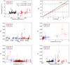 |
Fig. 6 Top left panel: scatter plot of frequency vs. relative speed for Encke in HI-1A (black dots), and ISON in HI-1A (red) and HI-2A (blue). The slope of the fitting line is related to the Strouhal number. Top right panel: extrapolation of the Strouhal number with respect to the coma size L. Middle panels: Strohual numbers of each data point vs. time (left panel), and vs. the oscillation amplitude (right panel). Bottom panels: S t vs. the frequency f (left panel), and vs. the relative speed V (right panel). |
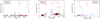 |
Fig. 7 Variation of the oscillation amplitude vs. time, vs. period of the oscillations (the inset plot magnifies the inner region containing Encke and ISON’s data points in HI-1A), and vs. distance along the cometary tail. In black Encke’s data points, in red and blue ISON’s data points from HI-1A and HI-2A, respectively. |
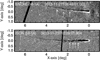 |
Fig. 8 Snapshots of Encke and ISON from HI-1A with some small-scale perturbations of the tails highlighted by the white arrows. |
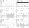 |
Fig. 9 Numerical solutions of the differential Eq. (3) for different types of ideal solar wind profiles. |
Movies
Movie for Fig. 1 Access Supplementary Material
Movie for Fig. 2 Access Supplementary Material
Movie for Fig. 3 Access Supplementary Material
Movie for Fig. 4 Access Supplementary Material
Acknowledgements
STEREO-HI data are courtesy of the UK Solar System Data Centre. VV and GN acknowledge support from the URSS scheme at the University of Warwick. GN and VB acknowledge support of the CGAUSS (Coronagraphic German and US Solar Probe Plus Survey) project for Parker Solar Probe/WISPR by the German Space Agency DLR under grant 50 OL 1601. VMN acknowledges the funding by STFC consolidated grant ST/P000320/1. K.B. was supported by the NASA-funded Sungrazer Project. G.N. would also thank the members of CFSA at the University of Warwick and the Astrophysics group at the University of Calabria for useful comments and discussion after the presentation of this subject.
References
- Aschwanden, M. J., Nitta, N. V., Wuelser, J.-P., & Lemen, J. R. 2008, ApJ, 680, 1477 [NASA ADS] [CrossRef] [Google Scholar]
- Battams, K., & Knight, M. M. 2017, Phil. Trans. R. Soc. A, 375, 20160257 [NASA ADS] [CrossRef] [Google Scholar]
- Bewsher, D., Brown, D. S., Eyles, C. J., et al. 2010, Sol. Phys., 264, 433 [NASA ADS] [CrossRef] [Google Scholar]
- Biesecker, D. A., Lamy, P., St. Cyr, O. C., Llebaria, A., & Howard, R. A. 2002, Icarus, 157, 323 [NASA ADS] [CrossRef] [Google Scholar]
- Biskamp, D. 2003, Magnetohydrodynamic Turbulence (Cambridge, UK: Cambridge University Press), 310 [Google Scholar]
- Brueckner, G. E., Howard, R. A., Koomen, M. J., et al. 1995, Sol. Phys., 162, 357 [NASA ADS] [CrossRef] [Google Scholar]
- DeForest, C. E., Matthaeus, W. H., Howard, T. A., & Rice, D. R. 2015, ApJ, 812, 108 [NASA ADS] [CrossRef] [Google Scholar]
- Downs, C., Linker, J. A., Mikić, Z., et al. 2013, Science, 340, 1196 [NASA ADS] [CrossRef] [Google Scholar]
- Dynnikova, G. Y., Dynnikov, Y. A., & Guvernyuk, S. V. 2016, Phys. Fluids, 28, 054101 [NASA ADS] [CrossRef] [Google Scholar]
- Foullon, C., Verwichte, E., Nakariakov, V. M., Nykyri, K., & Farrugia, C. J. 2011, ApJ, 729, L8 [NASA ADS] [CrossRef] [Google Scholar]
- Gruszecki, M., Nakariakov, V. M., van Doorsselaere, T., & Arber, T. D. 2010, Phys. Rev. Lett., 105, 055004 [NASA ADS] [CrossRef] [PubMed] [Google Scholar]
- Howard, R. A., Moses, J. D., Vourlidas, A., et al. 2008, Space Sci. Rev., 136, 67 [NASA ADS] [CrossRef] [Google Scholar]
- Johnson, S. 2004, Eur. J. Mech. B Fluids, 23, 229 [NASA ADS] [CrossRef] [Google Scholar]
- Jones, G. H., Balogh, A., & Horbury, T. S. 2000, Nature, 404, 574 [NASA ADS] [CrossRef] [Google Scholar]
- Kaiser, M. L. 2005, Adv. Space Res., 36, 1483 [NASA ADS] [CrossRef] [Google Scholar]
- Keane, J. V., Milam, S. N., Coulson, I. M., et al. 2016, ApJ, 831, 207 [NASA ADS] [CrossRef] [Google Scholar]
- Kivelson, M. G., & Russell, C. T. 1995, Introduction to Space Physics (Cambridge, UK: Cambridge University Press), 586 [Google Scholar]
- Knight, M. M., & Battams, K. 2014, ApJ, 782, L37 [NASA ADS] [CrossRef] [Google Scholar]
- Knight, M. M., Weaver, H. A., Fernandez, Y. R., et al. 2012, in LPI Contributions, Asteroids, Comets, Meteors 2012, 1667, 6409 [NASA ADS] [Google Scholar]
- Lee, H., Moon, Y.-J., & Nakariakov, V. M. 2015, ApJ, 803, L7 [NASA ADS] [CrossRef] [Google Scholar]
- Malara, F., Einaudi, G., & Mangeney, A. 1989a, J. Geophys. Res., 94, 11805 [NASA ADS] [CrossRef] [Google Scholar]
- Malara, F., Einaudi, G., & Mangeney, A. 1989b, J. Geophys. Res., 94, 11813 [NASA ADS] [CrossRef] [Google Scholar]
- Markwardt, C. B. 2009, in Astronomical Data Analysis Software and Systems XVIII, ed. D. A. Bohlender, D. Durand, & P. Dowler, ASP Conf. Ser., 411, 251 [NASA ADS] [Google Scholar]
- McCauley, P. I., Saar, S. H., Raymond, J. C., Ko, Y.-K., & Saint-Hilaire, P. 2013, ApJ, 768, 161 [NASA ADS] [CrossRef] [Google Scholar]
- Nakariakov, V. M., & Roberts, B. 1995, Sol. Phys., 159, 213 [NASA ADS] [CrossRef] [Google Scholar]
- Nakariakov, V. M., Aschwanden, M. J., & van Doorsselaere T. 2009, A&A, 502, 661 [NASA ADS] [CrossRef] [EDP Sciences] [Google Scholar]
- Odstrcil, D. 2003, Adv. Space Res., 32, 497 [CrossRef] [Google Scholar]
- Ponta, F. L., & Aref, H. 2004, Phys. Rev. Lett., 93, 084501 [NASA ADS] [CrossRef] [Google Scholar]
- Ramanjooloo, Y. 2015, PhD Thesis, (University College London) [Google Scholar]
- Sakamoto, H., & Haniu, H. 1990, ASME Trans. J. Fluids Eng., 112, 386 [NASA ADS] [CrossRef] [Google Scholar]
- Schrijver, C. J., Brown, J. C., Battams, K., et al. 2012, Science, 335, 324 [NASA ADS] [CrossRef] [Google Scholar]
- Sekanina, Z., & Kracht, R. 2014, ArXiv e-prints [arXiv:1404.5968] [Google Scholar]
- Thompson, W. T., & Wei, K. 2010, Sol. Phys., 261, 215 [NASA ADS] [CrossRef] [Google Scholar]
- Verma, M. K. 1996, J. Geophys. Res., 101, 27543 [NASA ADS] [CrossRef] [Google Scholar]
- Vourlidas, A., Davis, C. J., Eyles, C. J., et al. 2007, ApJ, 668, L79 [NASA ADS] [CrossRef] [Google Scholar]
Set of integrated software libraries and system utilities based on the Interactive Data Language (IDL): http://www.lmsal.com/solarsoft/.
Spacecraft, Planet, Instrument, Camera-Matrix, Events.
All Figures
|
Fig. 1 Running difference images of Encke and ISON from STEREO-A/HI-2 (left panel) and HI-1 (middle panel). Orbits of comets Encke (yellow line) and ISON (red line) in the Heliocentric-Aries-Ecliptic (HAE) coordinate system (right panel). Dashed lines indicate where the trajectory is below the ecliptic plane. The Earth is represented by the green dot (with the associated orbit dashed line style), while STEREO-A and B are shown with the red and blue dots, respectively. For reference, the position of the inner planets is also shown. The corresponding animations for each panel are available online. |
| In the text | |
|
Fig. 2 Left panels: variation of the distance from the Sun (top panel) for Encke (black) and ISON (red), and from STEREO-A in AU (bottom panel). Continuous lines mark the time intervals when the comets are visible in the HI-1 FoV, dotted lines the opposite. The blue dashed line in the bottom panel indicates the STEREO A-Sun distance, which is a reference line to visualise when the comets are behind or in front of the plane-of-sky. Right panels: orbital speed of the comets (top panel), and variation of the latitude in the Helio-Centric-Inertial (HCI) coordinate system (bottom panel). |
| In the text | |
|
Fig. 3 Time-distance maps (top panels), example of intensity profiles with related fittings (middle panels), and L vs. time (bottom panels) for Encke and ISON’s halo with HI-1A. |
| In the text | |
|
Fig. 4 Top left panel: solar wind speed on the solar equatorial plane provided by ENLIL. Earth’s position is fixed and represented by a green dot, while STEREO A and B are shown with red and blue dots, respectively. The trajectories of Encke and ISON projected on this plane are shown in orange and red, respectively, with some dots showing the positions of the comets with an interval of four days between 10 Nov and 4 Dec. The corresponding movie is available online. Top right panel: projected radial direction from the Sun, the projected direction of the orbital speed for Encke (red), and the resulting vectors V (yellow) determined as a vectorial sum between the solar wind VSW and the comet speed VC vectors. For a solar wind speed of 400 km s−1, the projected direction of V almost coincides with the tail direction. Bottom left panels: time-distance maps for Encke and ISON showing the inclination of the tail (the bright feature) with respect to the projected radial direction, and compared for different profiles of the aberration angle. In one case, we show the behaviour of the aberration angle profile for Encke assuming a sinusoidally variable solar wind with mean value of 400 km s−1, amplitude of 50 km s−1, and period of 12 h. Bottom right panel: plot of the relative speed magnitude V vs. time of observations assuming a constant and radial solar wind speed of 400 km s−1. |
| In the text | |
|
Fig. 5 Top panels: time-distance maps for Encke and ISON in HI-1A and HI-2A with showing the manually determined data points tracking the oscillations. Middle and bottom panels: sequences of 10 consecutive frames for Encke and ISON with some sinusoids indicating propagating waves along the tail. Values of amplitude, wavelength, and phase of the oscillations are reported on each single frame. The time-steps in min from the first frame of the sequence are shown on the top horizontal axis for each frame. |
| In the text | |
|
Fig. 6 Top left panel: scatter plot of frequency vs. relative speed for Encke in HI-1A (black dots), and ISON in HI-1A (red) and HI-2A (blue). The slope of the fitting line is related to the Strouhal number. Top right panel: extrapolation of the Strouhal number with respect to the coma size L. Middle panels: Strohual numbers of each data point vs. time (left panel), and vs. the oscillation amplitude (right panel). Bottom panels: S t vs. the frequency f (left panel), and vs. the relative speed V (right panel). |
| In the text | |
|
Fig. 7 Variation of the oscillation amplitude vs. time, vs. period of the oscillations (the inset plot magnifies the inner region containing Encke and ISON’s data points in HI-1A), and vs. distance along the cometary tail. In black Encke’s data points, in red and blue ISON’s data points from HI-1A and HI-2A, respectively. |
| In the text | |
|
Fig. 8 Snapshots of Encke and ISON from HI-1A with some small-scale perturbations of the tails highlighted by the white arrows. |
| In the text | |
|
Fig. 9 Numerical solutions of the differential Eq. (3) for different types of ideal solar wind profiles. |
| In the text | |
Current usage metrics show cumulative count of Article Views (full-text article views including HTML views, PDF and ePub downloads, according to the available data) and Abstracts Views on Vision4Press platform.
Data correspond to usage on the plateform after 2015. The current usage metrics is available 48-96 hours after online publication and is updated daily on week days.
Initial download of the metrics may take a while.