| Issue |
A&A
Volume 615, July 2018
|
|
|---|---|---|
| Article Number | A70 | |
| Number of page(s) | 12 | |
| Section | Galactic structure, stellar clusters and populations | |
| DOI | https://doi.org/10.1051/0004-6361/201732277 | |
| Published online | 17 July 2018 | |
The dynamically selected stellar halo of the Galaxy with Gaia and the tilt of the velocity ellipsoid
Kapteyn Astronomical Institute, University of Groningen,
PO Box 800,
9700
AV Groningen,
The Netherlands
e-mail: This email address is being protected from spambots. You need JavaScript enabled to view it.
Received:
10
November
2017
Accepted:
5
March
2018
Abstract
Aims. We study the dynamical properties of halo stars located in the solar neighbourhood. Our goal is to explore how the properties of the halo depend on the selection criteria used to define a sample of halo stars. Once this is understood, we proceed to measure the shape and orientation of the halo’s velocity ellipsoid and we use this information to put constraints on the gravitational potential of the Galaxy.
Methods. We use the recently released Gaia DR1 catalogue cross-matched to the RAVE dataset for our analysis. We develop a dynamical criterion based on the distribution function of stars in various Galactic components, using action integrals to identify halo members, and we compare this to the metallicity and to kinematically selected samples.
Results. With this new method, we find 1156 stars in the solar neighbourhood that are likely members of the stellar halo. Our dynamically selected sample consists mainly of distant giants on elongated orbits. Their metallicity distribution is rather broad, with roughly half of the stars having [M/H] ≥ −1 dex. The use of different selection criteria has an important impact on the characteristics of the velocity distributions obtained. Nonetheless, for our dynamically selected and for the metallicity selected samples, we find the local velocity ellipsoid to be aligned in spherical coordinates in a Galactocentric reference frame. This suggests that the total gravitational potential is rather spherical in the region spanned by the orbits of the halo stars in these samples.
Key words: Galaxy: kinematics and dynamics / Galaxy: structure / Galaxy: halo / solar neighborhood
© ESO 2018
1 Introduction
The study of our Galaxy offers a unique opportunity to unravel how galaxies in general came about. In the Milky Way, the oldest stars that we see today formed from very pristine material and likely still retain the memory of the physical and dynamical conditions of the interstellar medium where they formed more than 10 Gyr ago (e.g. Eggen et al. 1962; Helmi 2008, for a review of the subject). These “fossil” stars are part of the so-called stellar halo of the Galaxy, however their number is just a small fraction of the population of stars that are present in the Galactic disc(s). Also near the Sun, their spatial density is negligible. The present paper revolves on how to find these “precious” stars in the context of the ongoing “golden era” of Galactic surveys, which is characterized by the advent of the revolutionary astrometric mission Gaia and vast spectroscopic surveys such as the RAdial Velocity Experiment (RAVE; Steinmetz et al. 2006), the Apache Point Observatory Galactic Evolution Experiment (APOGEE; Majewski et al. 2017), and in the near future WEAVE (Dalton et al. 2012) and 4MOST (de Jong et al. 2012).
Halo stars are also interesting from the dynamical point of view because they have elongated orbits that probe the outer regions of the Galaxy, and thus can be used to study the total gravitational potential of the Milky Way, including its dark matter distribution. One measurable property that is often used to constrain the shape of the dark matter halo is the orientation of the stellar velocity ellipsoid (e.g. Lynden-Bell 1962; Ollongren 1962). The most recent estimates of the so-called tilt of the stellar velocity ellipsoid of both the Galactic disc (Siebert et al. 2008; Smith et al. 2012; Büdenbender et al. 2015) and the stellar halo (Smith et al. 2009b; Bond et al. 2010; Carollo et al. 2010; Evans et al. 2016) find that the stellar velocity ellipsoid is aligned in a Galacto-centric spherical reference frame and that it is elongated towards the Galactic centre. Although there has been some debate on its actual constraining power (e.g. Binney & McMillan 2011), recently An & Evans (2016) have established that the shape of the total gravitational potential can indeed be locally constrained.
The quest for stars in the Galactic halo is crucially influenced by the prior knowledge that we put in the criteria to select these objects. For instance, if we want to find the oldest stars in the Galaxy, we might select stars by their scarcity of metals and we may find that some of these stars move on high angular momentum near circular planar orbits that are more typical of the disc (e.g. Norris et al. 1985). On the other hand, if we want to find stars with halo-like orbits, we might select the fastest moving stars in a catalogue and encounter not only low-metallicity stars, but also more metal-rich stars (e.g. Morrison et al. 1990; Ryan & Norris 1991). Such metallicity selected or kinematically selected samples are biased by construction and this may affect the study of the structural properties of the Galactic stellar halo. In general, it may be preferable to identify stars using distribution functions. For example, if the current position in the phase-space of a star is actually known, then its full orbit can be reconstructed (given a Galactic potential), and the impact of such biases can thus be limited by analysing the stars that move far from the disc.
In this paper we use the distribution function approach in order to distinguish stars in the different Galactic components by their dynamics. We mainly use the fact that stars in the Galactic disc(s) are on low-inclination, high angular momentum orbits, while those in the stellar halo tend to have significantly different dynamics being on low angular momentum, eccentric, inclined orbits. This will allow us to identify halo stars in the recently released TGAS dataset (which is part of the first Gaia data release, Gaia Collaboration 2016) in combination with the spectroscopic information coming from the RAVE survey. We will then use the resulting metallicity and kinematically unbiased sample of halo stars to measure the tilt of the halo’s velocity ellipsoid near the Sun.
The paper is organized as follows. In Sect. 2 we describe the catalogue of stars considered from the TGAS and RAVE samples. In Sect. 3 we present the new method used to identify halo stars given their dynamics. In Sect. 4 we apply these selection criteria to the stars common to TGAS and RAVE. We then study the kinematics and metallicity distributions of the local stellar halo and compare our results to those obtained using other selection criteria. We also measure in Sect. 4 the tilt of the velocity ellipsoid and discuss the implicationson the mass models of the Galaxy. In Sect. 5 we present a summary of our results and conclusions.
2 Data: the TGAS-RAVE catalogue
The dataset used in this paper comes from the intersection of the TGAS sample produced by the Gaia mission in its first data release (Gaia Collaboration 2016) and the stars observed by the RAVE Survey (DR5; Kunder et al. 2017). We use the TGAS positions on the sky and proper motions, together with their uncertainties and mutual correlation. This sample has about two million stars with magnitudes 6 ≲ G < 13. The radial velocities and their uncertainties are from the RAVE DR5 catalogue, while stellar parameters, such as surface gravities and metallicities, and their uncertainties are from the updated RAVE pipeline by McMillan et al. (2017). For the parallaxes ϖ, we consider both the trigonometric values in the TGAS catalogue and the spectro-photometric values derived by McMillan et al. (2017), and we use for each star the one that has the smallest relative error Δ ϖ∕ϖ, with Δ ϖ the parallax uncertainty. The new determination by McMillan et al. (2017) significantly improves the accuracy of the parallaxes of stars common to TGAS and RAVE since it uses the trigonometric TGAS parallaxes as priors to further constrain those derived spectro-photometrically with the method of Burnett & Binney (2010).
From the RAVE DR5 catalogue we select only the stars satisfying the following quality criteria:
- (i)
signal-to-noise of the RAVE spectrum S/N ≥ 20;
- (ii)
Tonry & Davis (1979) correlation coefficient >10;
- (iii)
flag for stellar parameter pipeline Algo_Conv_K≠1;
- (iv)
error on radial velocity ϵRV ≤ 8 km s−1
(see Kordopatis et al. 2013; Helmi et al. 2017). This ensures that the stellar parameters, such as surface gravity, effective temperature, and metallicity, and thus also the absolute magnitude, distance, and parallax, are well constrained by the observed spectrum. We use this subset of the RAVE stars to make our own cross-match with TGAS based on the Tycho-2 IDs, and find 185 955 stars in common. We further require that
 (1)
(1)
where ϖTGAS is the measured TGAS parallax and ϖRAVE is the maximum likelihood value of the parallax, and ΔϖTGAS and Δ ϖRAVE are their uncertainties. This gives 178 067 stars, of which 19 273 have ΔϖTGAS∕ϖTGAS < ΔϖRAVE∕ϖRAVE, thus we compute the distance to the star from the trigonometric TGAS parallax as d = 1∕ϖTGAS; instead, for the remaining 158 794 stars, we use the distance estimate from McMillan et al. (2017). Although caution is required (e.g. Arenou & Luri 1999; Bailer-Jones 2015; Astraatmadja & Bailer-Jones 2016), recent analyses have shown that the reciprocal ofthe parallax is actually the most accurate distance estimator for stars with relative parallax error smaller than a few tens of percent (Binney et al. 2014; Schönrich & Aumer 2017). This is probably preferable than, for example, the use of a prior in the form of an exponential for the intrinsic spatial distribution of halo stars (which are known to follow a power-law distribution).
More than 90% of the halo stars we identify in our analyses below have parallaxes derived as in McMillan et al. (2017) since their relative parallax error is smaller than that given by TGAS. Moreover, more than 90% of the halo stars have Δϖ∕ϖ > 0.1, thus the cut at 30% relative parallax error (Eq. (1)) proves to be good balance between number of halo stars identified and accuracy. We also assess the robustness of the results in this paper against different estimates of the spectro-photometric parallaxes by repeating the analysis on a sample of stars with parallaxes from the RAVE DR5 public catalogue (Kunder et al. 2017); in Appendix A we show that all of our main results are not significantly altered by this choice.
Finally, we exclude stars with d < 0.1 kpc to reduce contamination from the local stellar disc. Our final catalogue is thus composed of 175 006 stars.
3 Identification of a halo sample
3.1 Summary of the method
The main idea of our identification method is to distinguish Galactic components (thin disc, thick disc, and stellar halo) on the basis of the orbits of the stars. For instance, we consider a star on a very elongated or highly inclined orbit is likely to be from the stellar halo, whereas a star on an almost circular planar orbit is likely to be part of the thin disc. We do not use any criterion based on metallicities or colours, or directly dependent on the velocities of the stars.
We characterize the orbits of stars by computing a complete set of three integrals of motion, which we choose to be the actions J in an axisymmetric potential. Each dynamical model that we use for each Galactic component is specified by the distribution function (hereafter DF) f, which is a function that gives the probability of finding a star at a given point in phase space (see e.g. Binney & Tremaine 2008). We formalize this via the following procedure:
- (i)
We define a DF fcompfor each Galactic component. These are functions of the actions Jof a star (hence its orbit); they add up to the total DF of the Galaxy
 (2)
(2)and we use them as error-free likelihoods for the membership estimation of each component;
- (ii)
We compute the self-consistent total gravitational potential Φ solving Poisson’s equation for the total density (see e.g. Binney 2014) ρ(x) = ∫ dv fgalaxy(J);
- (iii)
we characterize the orbits of stars by defining a canonical transformation from position-velocity to action-angle coordinates, which depends on the total gravitational potential,
 (3)
(3)and we compute it with the “Stäckel Fudge” following Binney (2012);
- (iv)
for each star, we sample the error distribution in the space of observables assuming it is a six-dimensional multivariate normal with mean and covariance as observed. We apply coordinate transformations to these samples, from observed to (x, v) and thento (θ, J) (Eq. (3)), in order to estimate the error distribution in action space γ(J);
- (v)
we define the likelihood
 that a star i belongs to a given component η by convolving the resulting error distribution in action space with the DF of that component as in (i), hence
 (4)
(4)
3.2 Actions and distribution function of the Galaxy
Actions J are the most convenient set of integrals of motion in galaxy dynamics, one of the reasons being that they are adiabatic invariants. In an axisymmetric potential, the first action JR quantifies the extent of the radial excursion of the orbit, the second Jϕ is simply the component of the angular momentum L along the z-direction (which is perpendicular to the symmetry plane), while the third action Jz quantifies the excursions in that direction.
In general actions are not easy to compute except for separable gravitational potentials. Nonetheless, many methods have been developed in recent years for general axisymmetric and triaxial potentials and they all yield consistent results for the cases of interest in galactic dynamics (for a recent review of the methods see Sanders & Binney 2016). Throughout the paper we adopt the algorithm devised by Binney (2012) to compute J = J(x, v) for all the stars in our sample, given a Galactic potential Φ. In short, theso-called Stäckel Fudge algorithm computes the actions in a separable Stäckel potential which is a local approximation to the Galactic potential Φ in the region explored by the orbit. While there is, in principle, no guarantee that a global set of action-angle variables exists for the given potential Φ, such a local transformation can always be found.
We thenfollow Piffl et al. (2014, see also Cole & Binney 2017) and define the DF of the Galaxy to be an analytic function of the three action integrals J = (JR, Jϕ, Jz), as the superposition of three components: the thin disc, thick disc, and stellar halo. We write the final DF as
 (5)
(5)
The parameters of the quasi-isothermal DFs of the discs are described in Piffl et al. (2014), and have been constrained using the RAVE dataset and for the purpose of this paper, are kept fixed. The mass of each component is  , and they add up to Mgal = 4.2 × 10¹⁰M⊙. Since we are interested in stars in the solar neighbourhood, there is no need to model the distribution in phase-space of the central regions of the Galaxy, within ≲5 kpc, thus in the final model we only include an axisymmetric bulge as an external, fixed component in the total potential. Modelling the effect of the bar on the orbits of stars in the solar neighbourhood as well goes beyond the scope of this paper.
For the stellar halo we assume the DF is a power-law function of the actions,
![Mathematical equation: \begin{equation*}{f_{\textrm{halo}}}(\textbf{J})\equiv{m_{\textrm{halo}}}\left[1+g(\textbf{J})/J_0\right]^{\beta_{\ast}}, \end{equation*}](/articles/aa/full_html/2018/07/aa32277-17/aa32277-17-eq8.png) (6)
(6)
where mhalo is a constant such that Mhalo = 5 × 10⁸M⊙, β* = −4, and J0 = 500 kpc km s−1, and where
 (7)
(7)
is a homogeneous function of the three actions. For (δϕ, δz) = (1, 1), the model is nearly spherical in the solar neighbourhood. The constant J0 serves to produce a core in the innermost R ≲ 1.5 kpc of the halo and it has the only purpose of making the stellar halo mass finite.
This choice for the DF generates models with density distributions which are also power laws (Posti et al. 2015; Williams & Evans 2015); for our choice of β* the density distribution of the halo follows roughly ρ ∝ r−3.5. This yields a reasonable description for the stellar halo in the solar neighbourhood (where our dataset is located), but does not take into account the possibility that the structure of the halo may change as a function of distance (e.g. Carollo et al. 2007; Deason et al. 2011; Das & Binney 2016; Iorio et al. 2018).
Our results are not very strongly dependent on the values chosen for the characteristic parameters of the DF in Eq. (6). We have tested our method i) with different geometries (spherical, as in our default, or flattened, which for (δϕ, δz) = (1∕2, 1) yields q = 0.7 at R0); ii) with different velocity distributions (isotropic or tangentially/radially anisotropic); iii) with different logarithmic slopes of the density distributions at R0 (from –2.5 to –3.5); and even iv) with different masses (from half to twice Mhalo). We found that more than 94% of stars identified as “halo” are in common for the different choices.
3.3 Gravitational potential
The Galactic potential that we use is made up of several massive components of two different kinds: i) static components and ii) DF components with self-gravity.
We have three components of the first kind, which we take from Piffl et al. (2014, Table 1 and their results for the dark halo): a gaseous disc, an oblate bulge, and an oblate dark matter halo. The gaseous disc is modelled as an exponential in both R and z, with scale-length Rd, g = 5.36 kpc and scale-height zd,g = 40 pc, a 4 kpc hole in the central region, and total mass of Mgas = 1010M⊙. The bulge is instead an oblate (q = 0.5) double power-law density distribution with scale radius of r0,b = 75 pc, exponential cut-off at rcut,b = 2.1 kpc, and total mass of Mbulge = 8.6 × 10⁹M⊙. The dark matter is distributed as a flattened (q = 0.8) halo (Navarro et al. 1996), truncated at the virial radius, with scale radius r0,DM = 14.4 kpc and virial mass of MDM = 1.3 × 10¹²M⊙.
Each stellar component of the Galaxy that we modelled with a DF has a contribution to the total gravitational potential Φ given by Poisson’s equation. Starting from an initial guess for the Galactic potential Φ0, which also contains the contributions from the static components, we compute the density distributions by integrating their DFs over the velocities and then, using Poisson’s equation, we compute the new total galactic potential Φ1. We use the iterative scheme suggested by Piffl et al. (2015) to converge (in ~ 5 iterations) to the total self-consistent gravitational potential Φ.
With this procedure the final model, specified by this gravitational potential and the galaxy DF given by Eq. (5), is self-gravitating, i.e. the stars are not merely treated as tracers of the potential.
3.4 Error propagation
To computethe actions (and their uncertainties) from the observables, we proceed as follows. We define a reference system centred on the Galactic Centre, where the z-axis is aligned with the disc’s angular momentum, x-axis is aligned with the Sun’s direction, and y-axis is positive in the direction of rotation. In this frame, the Sun is located at (–8.3, 0, 0.014) kpc with respect to the GalacticCentre and we assume a solar peculiar motion, with respect to the local standard of rest (LSR), of V⊙ = (11.1, 12.24, 7.25) km s−1 (Schönrich et al. 2010).
In order to get an estimate of the error distribution in action space, we start from the error distribution in the space ofobservables. We assume that this can be described by a six-dimensional multivariate normal distribution with the measurements as means, their uncertainties as standard deviations, and their mutual correlations as the normalized covariances. For the sky coordinates and velocities determined by TGAS (RA, Dec, μRA, μDec), we have estimates of their uncertainties and correlations, while the line-of-sight velocities vlos only have uncertainty estimates from RAVE, i.e. the correlations with the other coordinates are null. For those stars for which we take the parallax ϖTGAS we include correlations with the other TGAS coordinates in the covariance matrix, while for those for which we use the ϖRAVE we set them to be null.
We sample the resulting six-dimensional multivariate normal distribution of each star with 5000 discrete realizations, and convert each realization to the desired reference frame where we estimate the means, variances, and covariances. This completely specifies the error distribution in the new space if we further assume that there the uncertainties are also correlated Gaussians. We call γ[q, C(q)] the resulting multivariate distribution in the space of the new parameters q with covariance C (q) and we refer to it as γ(q).
3.5 Component membership estimation
As discussed earlier, the orbit of a star in a given gravitational potential is completely specified by the values of a complete set of isolating integrals of motion such as the action integrals. Suppose now we have characterized the orbit of a star by computing the actions, how do we evaluate the probability that a star belongs to one of the Galactic components?
We answer this question by computing the phase-space probability density of finding the given star with actions J for each of the three stellar components, i.e. we compute the value of the DF. Since we are interested in knowing which is the most likely component to which the star belongs, we can work with relative quantities and we can define likelihoods in terms of probability density ratios. In particular, we proceed by defining for each component η the likelihood
 (8)
(8)
where the subscript “ef” indicates that it is an error-free estimate. If for the component η
 (9)
(9)
then the probability of finding the star with actions J in that component is greater than in the other components.
For eachstar i, we estimate its error distribution in action space γi(J) starting from the error distribution of the observables as described in Sect. 3.4. We can take into account how measurement errors blur the estimate of the probability density of each stellar component by convolving the DFs of each component η with γi, hence
 (10)
(10)
If this estimator is
 (11)
(11)
and Pthreshold ≥ 1, then the probability that star i, with actions J and error distribution in action space γi, belongs to the component η is higher than for any of the other components. The condition given by Eq. (11) is the basis of our halo membership criteria.
4 Results for the local stellar halo
We now apply the method described in the previous section to our dataset. In order to have a prime sample of halo stars we used a more conservative Pη > Pthreshold, and Pthreshold = 10 proved to be a convenient choice. Out of the ~ 175 000 stars in our dataset we find 1156 likely to belong to the stellar halo1 (0.66%). Of these, 784 are found within d < 3 kpc.
In Fig. 1 we show the distribution of stars identified as halo in a projection of the action-space, namely on the Jϕ − JR plane, and we compare it to the distribution of all the other stars in the catalogue. The vast majority of the stars in the TGAS-RAVE catalogue are actually disc stars on nearly circular orbits, hence they mostly have high angular momentum (Jϕ ~ J⊙≃−2000 kpc km s−1, where J⊙ is the angular momentum of the Sun), low eccentricity (JR ~ 0), and typically stay close to the plane (Jz ~ 0). The halo stars, instead, have typically Jϕ ~ 0 and JR ≃ 500−1000kpc km s−1, meaning that they are on low angular momentum and elongated orbits. For completeness, in Fig. 1we also show the uncertainties on the action integrals that we estimate by computing the interval of 16th–84th percentiles of the resulting discrete samples obtained by propagating the measured error distribution in the observables (Sect. 3.4). The mean error on the radial action for this sample is Δ JR ~ 125kpc km s−1 (Δ JR∕JR ~ 26%), while that of the angular momentum is Δ Jϕ ~ 280kpc km s−1 (Δ Jϕ∕Jϕ ~ 17%) and that of the vertical action is Δ Jz ~ 80kpc km s−1 (Δ Jz∕Jz ~ 37%).
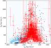 |
Fig. 1 Distribution of halo stars (red filled circles) in the angular momentum-radial action space. For comparison, we also plot all the stars in the sample (mostly disc stars) with cyan symbols and with a histogram of point density in the crowded region where orbits are nearly circular (JR ~ 0, Jϕ ~ J⊙). The cyan points at large JR and/or at small or retrograde Jϕ, although located in the region where the halo dominates, in practice have uncertainties that are too large and thus fail to pass the criterion given by Eq. (11); they are therefore not part of the dynamically selected halo. The yellow star marks the position of the Sun in this diagram. We show 16th–84th percentile error bars, computed as in Sect. 3.4, for all the halo stars with fractional error on JR smaller than 90%; instead, we plot as black empty circles the other halo stars for visualization purposes. |
4.1 Comparison samples
We now analyse the local kinematics and the metallicity distribution of the dynamically selected halo. We compare these distributions to those of samples obtained by applying two widely used selection criteria for halo stars: a selection based on metallicity and one based on kinematics.
4.1.1 Metallicity selected local stellar halo
A commonly used selection criterion for halo stars in the Galaxy is to assume that they are typically old and formed of low-metallicity material. The idea is then to identify as halo all the stars that are more metal-poor than a given threshold, typically a small percent of the solar metallicity.
For our comparison we use a sample of metallicity selected halo stars compiled as in Helmi et al. (2017), but using the distances to the stars from the updated pipeline by McMillan et al. (2017, Veljanoski et al., in prep.). The Galactic halo is defined as the component whose stars have metallicity [M∕H] ≤−1 dex (RAVE calibrated, see Zwitter et al. 2008). Since this metallicity threshold is not very strict, a second criterion is applied after a two-Gaussian decomposition of the sample is done; a star is said to belong to the halo if its velocity is more likely compatible with a normal distribution in (VX, VY, VZ) centred at VY ~ 20 km s−1 than with another centred at VY ~ 180 km s−1 (for more details, see Sect. 2.2 in Helmi et al. 2017). This sample has a total of 1217 stars, of which 713 are found closer than 3 kpc.
4.1.2 Kinematically selected local stellar halo
Halo stars are also commonly identified as the fastest moving stars with respect to the LSR. In particular, following Nissen & Schuster (2010), we define the kinematically selected stellar halo sample as being comprised of all the stars with |V −VLSR| > VLSR, where V = (VX, VY, VZ) is the star’s velocity in Galactocentric Cartesian coordinates and VLSR = (0, vLSR, 0) km s−1 is the velocity of the LSR (see also Bonaca et al. 2017). For the Galactic potential we use vLSR = 232 km s−1 (Sect. 3.3). The sample comprises a total of 1956 stars, of which 1286 are found closer than 3 kpc.
4.2 Properties of the different samples
As is clear from Fig. 2, where we plot the distribution of stellar surface gravities log g (as measured by RAVE) and distances d for the three samples considered here, most stars are distant giants. We do not see any significant bias or difference in the log g and d distributions (left and middle panels, respectively) in the three samples. The right panel of Fig. 2 shows the circularity lz for the samples and also includes the distribution for the whole TGAS-RAVE sample. We define the circularity lz of a star to be the ratio of its angular momentum to that of the circular orbit at the same energy Lcirc(E), i.e. lz = Jϕ∕Lcirc(E). Figure 2 shows that the proposed dynamical selection criteria successfully distinguishes halo stars from those in the disc (for which lz ~−1). We also note that the metallicity selected sample contains stars with orbits that are disc-like.
Very distant stars typically span different physical volumes than more closer ones. The complex TGAS-RAVE selection function likely yields a rather incomplete sample of stars at large distances, hence we will work with just a local sample of halo stars defined as those with d ≤ 3 kpc for most of the following discussion.
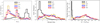 |
Fig. 2 Distribution of surface gravities (left panel), distances (middle panel), and circularities (right panel) of the stars in the dynamically selected (red), kinematically selected (blue), and metallicity selected (yellow) stellar halo. For comparison, we also plot in black the distribution of all the stars in the TGASxRAVE sample defined in Sect. 2. The circularities for the whole sample are shown on a 4x finer bin grid for visualization purposes. |
4.2.1 Local kinematics
In Galactocentric Cartesian coordinates (VX, VY, VZ) we define the Toomre diagram as the plane VY versus  . This is shown in Fig. 3 for the stars in the three selected halo samples. The kinematically selected halo is actually defined in this plane by the semi-circle |V −VLSR| = VLSR, which sets a sharp cut for the halo/non-halo stars (Fig. 3, middle panel). In both the dynamically and the metallicity selected samples there are, instead, a non-negligible number of stars in the region that would not be allowed by the kinematic criterion (respectively 18% and 22%). On the other hand, of the halo stars selected by kinematics there are 1204 stars that are more metal-rich than [M/H] = −1 dex, hence not belonging to the metallicity selected sample, and 1009 stars that are not selected dynamically because their measurement errors are too large to pass the condition defined by Eq. (11) with our strict threshold value. These two groups of stars are represented by the cyan points outside the semi-circle |V −VLSR| > VLSR in the right and left panels of Fig. 3, respectively.
The kinematic selection of halo stars produces unrealistic asymmetries in the plane of VY and  (Fig. 3). These asymmetries translate into similar features in the distribution of cylindrical Galactocentric velocities (vR, vϕ, vz), as shown in Fig. 4. While the histograms of the radial and azimuthal velocities of the kinematically selected halo appear quite asymmetric, the distributions for the dynamically selected halo are relatively symmetric, and are consistent with being Gaussian2.
In Fig. 5 we show the distributions of stars in the vR − vz and vR − vϕ planes for the threeselected samples. To better highlight the differences in the velocity distributions in the three cases, we bin velocity space uniformly and show in Fig. 6 the ratio of the fraction of stars per bin in the kinematically (or metallicity) selected halo to that of the dynamically selected halo. For the kinematically selected halo there is a significant lack of stars close to vϕ ~−200km s−1 and vR ~ 0, where most of the disc stars are (blue region in the top left panel of Fig. 6). This occurs because a kinematic selection is unable to distinguish between disc and halo stars in the region dominated by the disc. Such a selection also produces a peak in the Galactocentric radial velocity distribution at vR ≃ 180km s−1 (clearly visible as a high-contrast red region in the top left and bottom left panels of Fig. 6). By exploring their dynamical properties we believe that these stars are likely thick disc contaminants since they have little vertical action, about Jz ≃ 35kpc km s−1, which is close to the typical value of 10–20 kpc km s−1 for thick disc stars, and have typical circularity lz ≃−0.7, which is significantly closer to that of circular orbits (lz = −1) in comparison to the rest of the halo sample.
Conversely, in the region of velocity space dominated by the disc (vR, vϕ) ≃ (0, −200)km s−1, there is a significant concentration of stars in the case of a halo selected by metallicity (red region in the top right and bottom right panels of Fig. 6), indicating that there is still significant residual contribution of the metal-poor tail of the thick disc. The distribution of circularities (right panel of Fig. 2) also shows that there is indeed an excess of stars with lz ≲−0.8 with respect to the kinematically and dynamically selected samples. These stars contribute to making the distribution of vϕ for the metallicity selected halo not centred on zero, but on a slightly prograde value of  km s−1. If we remove stars with disc-like circularities (i.e. lz ≲−0.8) from this sample, then
  km s−1 (see also Deason et al. 2017; Kafle et al. 2017).
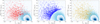 |
Fig. 3 Toomre diagram for the stars in our TGASxRAVE sample. In all the panels we plot all the stars with cyan symbols (and binned density). The red, blue, and yellow circles are respectively the stars in the dynamically selected, kinematically selected, and metallicity selected stellar halo. |
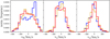 |
Fig. 4 One-dimensional distributions of the Galactocentric cylindrical velocities for stars in the dynamically selected (red), kinematically selected (blue), and metallicity selected (yellow) stellar halo. |
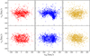 |
Fig. 5 Two-dimensional distributions of the Galactocentric cylindrical velocities for the dynamically selected (red), kinematically selected (blue), and metallicity selected (yellow) stellar halo stars. |
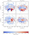 |
Fig. 6 Ratio of the normalized number of halo stars selected by kinematics (Nkin = Nbin, kin∕Ntot, kin, left panels) and by metallicity (Nmet = Nbin, met∕Ntot, met, right panels)to that of halo stars selected by dynamics (Ndyn = Nbin, dyn∕Ntot, dyn) in bins of thevR − vϕ (top panel) and vR − vz (bottom panel) velocity subspaces. Bins are coloured by the logarithm of the number counts ratio. |
4.2.2 Metallicity distribution
In Fig. 7 we show the RAVE calibrated metallicity distribution of the halo stars for the three samples. While the metallicity selected halo has a sharp edge at [M/H] ~−1 dex, which is the threshold for the selection, in the other two cases the distribution is peaked at [M/H] ~−0.5 dex and declines smoothly at higher metallicities reaching [M/H] ~ 0. In particular, we find 633 stars (55%) with [M/H] > −1 dex in the dynamically selected sample. These stars are all on highly elongated, low angular momentum orbits, and 215 of them (34%) are on retrograde orbits (see also Bonaca et al. 2017).
Figure 8 shows the distribution of the dynamically selected halo stars in the vϕ − [M/H] plane: the stars scatter around vϕ ~ 0 and [M/H] ~ −1 dex, with a slight but not significant tendency of retrograde motions at lower metallicities and vice versa (but see also Carollo et al. 2007; Beers et al. 2012; Kafle et al. 2017). This plot is, however, severely affected by measurement errors making trends difficult to discern because of the blurring induced especially by the uncertainties in azimuthal velocity. Moreover, we note here that even if we made sure that the error distributions in azimuthal velocity for our selection of halo stars do not deviate significantly from Gaussian (the interval of 16th–84th percentiles is close to two standard deviations), symmetric parallax (and/or distance) errors typically translate into asymmetric errors in vϕ (e.g. Ryan 1992; Schönrich et al. 2014), which complicates the understanding of the kinematics of the local stellar halo even further.
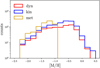 |
Fig. 7 Metallicity distribution (in number counts) for the dynamically selected (red), kinematically selected (blue), and metallicity selected (yellow) stellar halo samples. The RAVE calibrated metallicity [M/H] is from McMillan et al. (2017) and the typical uncertainty is ~ 0.2 dex. |
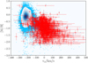 |
Fig. 8 Distribution of stars in the dynamically selected stellar halo (red) on the metallicity–azimuthal velocity space. For comparison, all stars in our TGASxRAVE sample are also shown (cyan). |
4.2.3 Distribution in action space
As shown inFig. 9, most of the halo stars in action space are centred around angular momenta Jϕ ~ 0, whereas disc stars have high angular momentum (Jϕ ~ J⊙) and low radial and vertical action (JR ~ Jz ~ 0). It is in this space that the dynamical selection acts, and as discussed before it depends on the phase space densities of each Galactic component. The ratio of the phase space densities of the halo fhalo to that of the discs fthin + fthick determines the number of stars assigned to either component in a given volume of action space. For instance, in a neighbourhood of (JR, Jϕ, Jz) = (0, J⊙, 0) the ratio of these phase space densities is so low that the probability of assigning a star to the stellar halo component is in fact negligible. The probability of halo membership given by Eq. (10) is also low for Jϕ < −600kpc km s−1 and Jz < 200kpc km s−1, where only a handful of stars satisfy the criteria. The likely consequence of this is that some genuine halo stars are missing from the dynamically selected sample and have been misclassified as thick disc stars. This is clearly dependent on the dynamical model of the Galaxy assumed for the selection and it is the reason why the distribution of dynamically selected halo stars is not symmetric (about Jϕ = 0) in the Jϕ − Jz projection, as can also be seen from a comparison to the metallicity selected sample.
For the catalogue of stars used in the present study the most important parameters determining the membership of stars at high angular momentum Jϕ and low vertical action are the parameters governing the vertical velocity dispersion of the thick disc: σz,0 and Rσ,z, the vertical velocity dispersion at the origin and the scale-length of its exponential decay, respectively. For instance, we find that with a smaller Rσ,z (which implies a thinner thick disc), the distribution of dynamically selected halo stars becomes significantly more symmetric in the Jϕ − Jz plane. However, Piffl et al. (2014) show that such a model provides an overall poorer fit to the observed velocity moments of all the RAVE stars, and thus it is unlikely to be the solution. We could in principle search the parameter space for the best model representing the RAVE data, which also yields a symmetric distribution of dynamically selected halo stars in action space, but it seems this exercise should be done when a larger, more complete dataset becomes available.
For comparison, we also show in Fig. 9 the distribution in action space for the halo stars selected by kinematics (middle panels) and metallicity (right panels). These plots show that in both cases there are many more halo stars in these two selections close to (JR, Jϕ, Jz) = (250, −1000, 100)kpc km s−1, in comparison to the dynamical selection. The stellar halo samples selected by kinematics and metallicity have, respectively, net angular momenta  and
and  kpc km s−1. On the other hand, we find no clear evidence of net rotation of the dynamically selected stellar halo (
 kpc km s−1). We note, however, that when we try to account for the halo stars that we might be missing at prograde Jϕ and Jz < 200kpc km s−1 (see Fig. 9), which we do by “mirroring” the retrograde stars with Jz < 200 hence making the Jϕ − Jz diagram symmetric at low vertical actions, we get a slightly prograde net rotation,
  kpc km s−1, which is marginally compatible with the rotation signal of the inner halo found by other authors (e.g. Deason et al. 2017).
Whether the stellar halo is rotating and whether it is made of several components with different kinematics are still matters of open debate. However, as we have just shown, it is important to realize that the conclusions we draw by analysing a sample of halo stars could (and often do) depend on the selection criteria used to define such a sample from a parent catalogue of stars in the Galaxy.
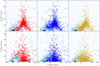 |
Fig. 9 Action space distribution of the dynamically selected (red), kinematically selected (blue), and metallicity selected (yellow) stellar halo stars. The yellow star marks the location of the Sun. |
4.3 Tilt of the velocity ellipsoid
We now turn to the characterization of the velocity dispersion tensor, also called velocity ellipsoid, of the local dynamically selected stellar halo, i.e.
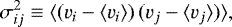 (12)
(12)
where  is the average of the quantity Q weighted by the phase-space DF (e.g. Binney & Tremaine 2008). The diagonal elements of this tensor are the velocity dispersions in the three orthogonal directions
  , while the off-diagonal elements represent the velocity covariances.
We employ a three-dimensional multivariate normal distribution  to describe the distribution of velocities of the stars in the stellar halo. This model is characterized by three mean orthogonal velocities
  and the (symmetric) velocity dispersion tensor σij, hence nine free parameters. The velocity correlations
 (13)
(13)
are then related to the angle given by
 (14)
(14)
where αij is the angle between the i-axis and the major axis of the ellipse formed by projecting the velocity ellipsoid on the i-j plane (see Binney & Merrifield 1998; Smith et al. 2009b, their Appendix A). In computing the posterior distributions for the model parameters, we also take into account measurement errors by defining the likelihood of a model as the convolution of  with the star’s error distribution γ(v). The latter is itself multivariate normal, hence their convolution results in a multivariate normal with mean the sum of the means and correlation the sum of the correlations. Given this likelihood, we finally sample the posterior distribution of the nine parameters with a Markov chain Monte Carlo method (MCMC; we use the python implementation by Foreman-Mackey et al. 2013) assuming uninformative (flat) priors for all the parameters3.
All our chains easily converge after the so-called burn-in phase, and the sampled posteriors are all limited with no correlation between any parameter couple. Thus, we derive a maximum likelihood value for all the parameters and estimate their uncertainties by computing the interval of 16th–84th percentiles of the posterior distributions. We summarize these results in both a cylindrical and a spherical reference frame in Table 1.
We find all the mean velocities to be consistent with zero, and the velocity dispersions we derive are broadly consistent with previous measurements (at the high end of the estimates of e.g. Chiba & Beers 2000; Bond et al. 2010; Evans et al. 2016). The velocity ellipsoid is mildly triaxial (σr > σθ ≳ σϕ) and the stellar halo is locally radially biased: the anisotropy parameter  . No significant correlation is found between the velocities in spherical coordinates, meaning that the halo’s velocity ellipsoid is aligned with a spherical reference frame, which has implications on mass models of the Galaxy (e.g. Smith et al. 2009b; Evans et al. 2016, and Sect. 4.3.1). We find a slightly larger vertical velocity dispersion (σz, σθ) than previous works; this is likely because of the dynamical selection that we have applied, which is meant to select only stars that are genuinely not moving in the disc and thus on orbits with typically large vertical oscillations. If we repeat the above analysis for the metallicity selected sample as in Helmi et al. (2017), we have an indication that this is happening, and obtain values that are more in line with previous estimates: (σr, σθ, σϕ) = (136 ± 6, 74 ± 4, 96 ± 5) km s−1. Also, the large vertical and the small azimuthal dispersion that we derive using our dynamically selected sample results in a velocity ellipsoid that is more elongated on the vertical, rather than the azimuthal direction (cf. Smith et al. 2009a; Bond et al. 2010; Evans et al. 2016).
In Fig. 10 we show the radial and vertical cylindrical velocities for the halo stars in our sample located at − 5≲ z∕kpc ≤−1 below the disc plane. There is a strong significant correlation between vR and vz with an angular slope of  deg, sometimes also called tilt-angle, which is estimated by marginalizing the posterior probability over all the other model parameters. It is interesting to compare this estimate to the value expected for a spherically aligned velocity ellipsoid, in which case αRz, sph = arctan(z∕R). For this subset of halo stars we derive αRz, sph = arctan(zmed∕Rmed) ≃−14.7 deg, where zmed ≃−2 kpc and Rmed ≃ 7.6 kpc are their median height and polar radius, respectively. The value obtained for αRz, sph is therefore consistent with our measurement of the tilt angle αRz.
To test whether the halo’s velocity ellipsoid is consistent with being spherically aligned for all z, we group the local (d ≤ 3 kpc) halo stars as a function oftheir z-height in four bins with roughly 185 stars each, and we use again a multivariate normal model to determine the tilt-angle αRz. In Fig. 11 we plot the most probable αRz and its uncertainty, as a function of z: there is a clear close-to-linear correlation in the sense that the tilt-angle is larger for samples of stars at greater heights above the Galactic plane. Such a correlation is precisely what is expected in the case of a spherical gravitational potential. An oblate/prolate Stäckel potential would result in a shallower/steeper αRz− z relation (seee.g. Eq. (17) in Büdenbender et al. 2015).
This result is surprisingly robust against different selection criteria used to identify halo stars. In the right panel of Fig. 11 we show, for instance, αRz as a function of z for the metallicity selected halo. Furthermore, in this case we find that αRz increases almost linearly with z, consistently with a model in which the velocity ellipsoid is everywhere spherically aligned. This indicates that the resulting velocity ellipsoid has a similar orientation which truly reflects the shape of the underlying total gravitational potential, even though selecting stars by their orbits or by metallicity yields somewhat different local velocity distributions for the halo (see Sect. 4.2.1). These results are also robust to different distance cuts.
Parameters of the local velocity ellipsoid for the dynamically selected halo.
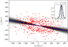 |
Fig. 10 Distribution of stars with − 5 ≲ z∕kpc ≤−1 in the dynamically selected stellar halo on the vR–vz subspace. Each black line represents the orientation of the velocity ellipsoid in this subspace as given by one sample in the MCMC chain. The inset shows the marginalized distribution of the angular slope of the black lines (tilt-angle). The blue line marks the expected orientation for a spherically aligned velocity ellipsoid. |
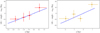 |
Fig. 11 Tilt-angle αRz as a function of height above the Galactic plane for the dynamically selected stellar halo (red circles, left panel) and the metallicity selected stellar halo (yellow circles, right panel). Each bin in z contains roughly the same number of stars (≃185 and ≃ 175 respectively for the two halos). The value of αRz and its uncertainty are estimated using a multivariate normal model as in Sect. 4.3, while the error bars in z indicate the 16th–84th percentile of the z distribution in that bin. The blue solid line indicates a model in which the halo’s velocity ellipsoid is aligned with the spherical coordinates. |
4.3.1 Implications for mass models of the Galaxy
The measurement of the orientation of the velocity ellipsoid of the stellar halo yields crucial insights on the overall gravitational potential of the Galaxy. While its axis ratios are related to the halo’s anisotropy and hence possibly to its formation history, at each point in space the orientation of the halo’s velocity ellipsoid is directly related to the shape of the total gravitational potential. For example, it has long been known that if the potential is separable in a given coordinate system, then its velocity ellipsoid is oriented along that coordinate system (e.g. Eddington 1915; Lynden-Bell 1962), but recently it has been shown that the contrary also holds, i.e. if the velocity ellipsoid is everywhere aligned with a given coordinate system, then the potential is separable in those coordinates (Evans et al. 2016). The necessary and sufficient condition for the potential of a steady-state stellar system to be separable in some given Stäckel coordinates (q1, q2, q3), i.e. it is a Stäckel potential, can be rewritten using the Jeans equations as follows: If i) all the velocity dispersions in a given orthogonal frame are different; ii) all the second-order mixed moments of the velocity vanish, ⟨vi vj⟩ = 0 for i≠ j; and iii) all fourth-order mixed moments with odd powers vanish,  , where l + m + n = 4 and at least one of l, m, n is odd (An & Evans 2016). For our dynamically selected halo sample, the correlation coefficients ρij with i≠ j (Eq. (13)), which are the second-order mixed velocity moments normalized to the respective velocity dispersions, are indeed compatible with being null in spherical coordinates. We also compute the fourth-order moments numerically4 and we derive fourth-order correlation coefficients by normalizing them by the respective velocity dispersions (squared), as in Eq. (13). We compute their uncertainties using the Monte Carlo samples. We find values no higher than 0.05± 0.06 for the normalized mixed moments with odd powers in velocity and of the order of 0.33± 0.06 for the normalized mixed moments of the type
  .
.
These results indicate that at least locally the stellar halo of the Galaxy respects the conditions of the theorem by An & Evans (2016), hence suggesting that the total Galactic potential may be separable in spherical coordinates. This is intriguing, since the only axisymmetric potentials which yield a finite mass for the Galaxy and are separable in spherical coordinates are the spherical potentials (e.g. Smith et al. 2009b). We note, however, that it is also possible to construct physically plausible Galaxy models in which the velocity ellipsoid is locally aligned with the spherical coordinates even in an oblate (Binney & McMillan 2011) or a triaxial gravitational potential (Evans et al. 2016), hence no strong conclusions can be reached with a local halo sample like the one we are using here. On the other hand, in non-spherical potentials the misalignment of the velocity ellipsoid with the spherical coordinates is typically small only in a limited region of space and, intuitively, gets smaller when the potential is closer to spherical symmetry (Evans et al. 2016). Future Gaia data releases will probe unexplored regions of the Galactic stellar halo and will lead to a large increase in the size of samples of halo stars, therefore allowing us to put significant constraints on the geometry of the Galactic potential.
5 Conclusions
In this paper we have devised a novel method to select stars in the stellar halo of our Galaxy from a catalogue with measured positions and velocities. Our method involves characterizing the orbit of each star using its actions and then computing the probability that the star is a member of a given Galactic component employing a specified self-consistent dynamical model for the Galaxy. We have applied this method to the ~ 175 k stars found in the intersection of the TGAS and RAVE catalogues and we have used the DF-based dynamical model by Piffl et al. (2014). We have compared this dynamically based selection of halo stars with one based purely on kinematics and one based on metallicities. We summarize here the main findings of the paper:
- (i)
We find 1156 halo stars in the solar neighbourhood, a number comparable to those found using the two alternative selection methods.
- (ii)
The halo stars in our sample are typically distant giants on very elongated orbits; they are mostly more metal-poor than [M/H] ≲−0.5, but we find that roughly half of the sample has [M/H] ≥−1, in broad agreement with what is found for a kinematically selected sample.
- (iii)
The velocity distribution of the dynamically selected sample is reasonably Gaussian, with means
 km s−1 and dispersions of (σr, σθ, σϕ) = (142 ± 6, 89 ± 4, 74 ± 6) km s−1. A kinematically selected sample is affected by strong biases and is clearly non-Gaussian, while a sample based on metallicity is also well-fit by a multivariate normal distribution, but shows slightly positive prograde rotational motion; the velocity ellipsoid has a slightly different shape, with (σr, σθ, σϕ) = (136 ± 6, 74 ± 4, 96 ± 5) km s−1.
 - (iv)
Differences in the properties of the velocity distributions can be traced back to the criteria used by the different selection methods. A dynamically based method suppresses the contribution of stars that have close to thick disc-like orbits, while if based on metallicity these stars are selected provided they have [M/H] < −1 dex (which leads to a higher σϕ and a lower σθ).
- (v)
Despite these differences, for both the dynamical and the metallicity-based selection methods, the tilt angle of the stellar halo is robustly measured and is consistent with being spherically aligned.
- (vi)
All the second-order velocity mixed moments, together with all the fourth-order ones with odd velocity powers, are consistent with being null in volume probed by the catalogue, which suggests that the total gravitational potential of the Galaxy has to be locally close to spherical (An & Evans 2016).
The method described here can be easily extended to categorize a sample of stars for which at least one of the six-dimensional phase-space coordinates is missing. Given a dynamical model in the form of a distribution function f(J) we can always define membership probabilities as in Sect. 3.5 by replacing the value of the six-dimensional phase-space density fη (J) for each Galactic component η by its analogue obtained by marginalizing over the missing coordinate. In the near future Gaia will provide five-dimensional information for more than a billion stars in the Galaxy, but radial velocities will be available for just about 10% of the total, hence devising algorithms that can exploit the full extent of the information available already with the second Gaia Data Release is of vital importance.
Acknowledgements
We acknowledge financial support from a VICI grant from the Netherlands Organisation for Scientific Research (NWO). This work has made use of data from the European Space Agency (ESA) mission Gaia (http://www.cosmos.esa.int/gaia), processed by the Gaia Data Processing and Analysis Consortium (DPAC, http://www.cosmos.esa.int/web/gaia/dpac/consortium). Funding for the DPAC has been provided by national institutions, in particular the institutions participating in the Gaia Multilateral Agreement.
Appendix A Results with spectro-photometric distances from RAVE DR5
Here we summarize the results of the selection method described in this paper with regard to the catalogue of stars where parallaxes are either trigonometric from TGAS or spectro-photometric from the RAVE DR5 database (Kunder et al. 2017), determined with the method by Binney et al. (2014). In this case the stellar parameters, such as surface gravity and calibrated metallicity, are obtained from the DR5 pipeline, and not from the updated McMillan et al. (2017) estimate.
We get a final sample of 159 702 stars by applying the cuts described in Sect. 2.
The sample of dynamically selected halo stars (see Sect. 3.5) is composed of 743 stars, i.e. 0.46% of the total sample.
278 halo stars have [M/H] > −1 (37%), 128 of which are on retrograde orbits (46%); 105 halo stars (14%) are found at relatively low velocities |V −VLSR| < VLSR.
The mean velocities of the local (d < 3 kpc) dynamically selected stellar halo (estimated as in Sect. 4.3) are all consistent with being null. The velocity dispersions are (σr, σθ, σϕ) = (149 ± 6, 96 ± 4, 87 ± 5)km s−1 and the velocity correlation coefficients are (ρrθ, ρrϕ, ρϕθ) = (0.05 ± 0.06, −0.03 ± 0.06, 0.04 ± 0.06).
For the sample of halo stars at z ≤−1 kpc below the Galactic plane, we find a tilt-angle αRz = −15 ± 5 deg, consistent with the expectation for a spherically aligned velocity ellipsoid of αRz = arctan(zmed∕Rmed) = −16 deg.
References
- An, J., & Evans, N. W. 2016, ApJ, 816, 35 [NASA ADS] [CrossRef] [Google Scholar]
- Arenou, F., & Luri, X. 1999, in Harmonizing Cosmic Distance Scales in a Post-HIPPARCOS Era, eds. D. Egret & A. Heck, ASP Conf. Ser., 167, 13 [Google Scholar]
- Astraatmadja, T. L., & Bailer-Jones, C. A. L. 2016, ApJ, 832, 137 [NASA ADS] [CrossRef] [Google Scholar]
- Bailer-Jones, C. A. L. 2015, PASP, 127, 994 [NASA ADS] [CrossRef] [Google Scholar]
- Beers, T. C., Carollo, D., Ivezić, Ž., et al. 2012, ApJ, 746, 34 [NASA ADS] [CrossRef] [Google Scholar]
- Binney, J. 2012, MNRAS, 426, 1324 [NASA ADS] [CrossRef] [Google Scholar]
- Binney, J. 2014, MNRAS, 440, 787 [NASA ADS] [CrossRef] [Google Scholar]
- Binney, J., & McMillan, P. 2011, MNRAS, 413, 1889 [NASA ADS] [CrossRef] [Google Scholar]
- Binney, J., & Merrifield, M. 1998, Galactic Astronomy (Princetown: Princetown University Press) [Google Scholar]
- Binney, J., & Tremaine, S. 2008, Galactic Dynamics: Second Edition (Princetown: Princetown University Press) [Google Scholar]
- Binney, J., Burnett, B., Kordopatis, G., et al. 2014, MNRAS, 437, 351 [NASA ADS] [CrossRef] [Google Scholar]
- Bonaca, A., Conroy, C., Wetzel, A., Hopkins, P. F., & Kereš D. 2017, ApJ, 845, 101 [NASA ADS] [CrossRef] [Google Scholar]
- Bond, N. A., Ivezić, Ž., Sesar, B., et al. 2010, ApJ, 716, 1 [NASA ADS] [CrossRef] [Google Scholar]
- Büdenbender, A., van de Ven, G., & Watkins, L. L. 2015, MNRAS, 452, 956 [NASA ADS] [CrossRef] [Google Scholar]
- Burnett, B., & Binney, J. 2010, MNRAS, 407, 339 [NASA ADS] [CrossRef] [Google Scholar]
- Carollo, D., Beers, T. C., Lee, Y. S., et al. 2007, Nature, 450, 1020 [NASA ADS] [CrossRef] [PubMed] [Google Scholar]
- Carollo, D., Beers, T. C., Chiba, M., et al. 2010, ApJ, 712, 692 [NASA ADS] [CrossRef] [Google Scholar]
- Chiba, M., & Beers, T. C. 2000, AJ, 119, 2843 [NASA ADS] [CrossRef] [Google Scholar]
- Cole, D. R., & Binney, J. 2017, MNRAS, 465, 798 [NASA ADS] [CrossRef] [Google Scholar]
- Dalton, G., Trager, S. C., Abrams, D. C., et al. 2012, in Ground-based and Airborne Instrumentation for Astronomy IV, Proc. SPIE, 8446, 84460P [CrossRef] [Google Scholar]
- Das, P., & Binney, J. 2016, MNRAS, 460, 1725 [NASA ADS] [CrossRef] [Google Scholar]
- de Jong, R. S., Bellido-Tirado, O., Chiappini, C., et al. 2012, Ground-based and Airborne Instrumentation for Astronomy IV, Proc. SPIE, 8446, 84460T [Google Scholar]
- Deason, A. J., Belokurov, V., & Evans, N. W. 2011, MNRAS, 416, 2903 [NASA ADS] [CrossRef] [Google Scholar]
- Deason, A. J., Belokurov, V., Koposov, S. E., et al. 2017, MNRAS, 470, 1259 [NASA ADS] [CrossRef] [Google Scholar]
- Eddington, A. S. 1915, MNRAS, 76, 37 [NASA ADS] [CrossRef] [Google Scholar]
- Eggen, O. J., Lynden-Bell, D., & Sandage, A. R. 1962, ApJ, 136, 748 [NASA ADS] [CrossRef] [Google Scholar]
- Evans, N. W., Sanders, J. L., Williams, A. A., et al. 2016, MNRAS, 456, 4506 [NASA ADS] [CrossRef] [Google Scholar]
- Foreman-Mackey, D., Hogg, D. W., Lang, D., & Goodman, J. 2013, PASP, 125, 306 [CrossRef] [Google Scholar]
- Gaia Collaboration, (Brown, A. G. A., et al.) 2016, A&A, 595, A2 [NASA ADS] [CrossRef] [EDP Sciences] [Google Scholar]
- Helmi, A. 2008, A&ARv, 15, 145 [CrossRef] [Google Scholar]
- Helmi, A., Veljanoski, J., Breddels, M. A., Tian, H., & Sales, L. V. 2017, A&A, 598, A58 [NASA ADS] [CrossRef] [EDP Sciences] [Google Scholar]
- Iorio, G., Belokurov, V., Erkal, D., et al. 2018, MNRAS, 474, 2142 [NASA ADS] [CrossRef] [Google Scholar]
- Kafle, P. R., Sharma, S., Robotham, A. S. G., et al. 2017, MNRAS, 470, 2959 [NASA ADS] [CrossRef] [Google Scholar]
- Kordopatis, G., Gilmore, G., Steinmetz, M., et al. 2013, AJ, 146, 134 [NASA ADS] [CrossRef] [Google Scholar]
- Kunder, A., Kordopatis, G., Steinmetz, M., et al. 2017, AJ, 153, 75 [NASA ADS] [CrossRef] [Google Scholar]
- Lynden-Bell, D. 1962, MNRAS, 124, 95 [NASA ADS] [CrossRef] [Google Scholar]
- Majewski, S. R., Schiavon, R. P., Frinchaboy, P. M., et al. 2017, AJ, 154, 94 [NASA ADS] [CrossRef] [Google Scholar]
- Matijevič, G., Zwitter, T., Bienaymé, O., et al. 2012, ApJS, 200, 14 [NASA ADS] [CrossRef] [Google Scholar]
- McMillan, P. J., Kordopatis, G., Kunder, A., et al. 2017, MNRAS, 477, 5279 [Google Scholar]
- Morrison, H. L., Flynn, C., & Freeman, K. C. 1990, AJ, 100, 1191 [NASA ADS] [CrossRef] [Google Scholar]
- Navarro, J. F., Frenk, C. S., & White, S. D. M. 1996, ApJ, 462, 563 [NASA ADS] [CrossRef] [Google Scholar]
- Nissen, P. E., & Schuster, W. J. 2010, A&A, 511, L10 [NASA ADS] [CrossRef] [EDP Sciences] [Google Scholar]
- Norris, J., Bessell, M. S., & Pickles, A. J. 1985, ApJS, 58, 463 [NASA ADS] [CrossRef] [Google Scholar]
- Ollongren, A. 1962, Bull. Astron. Inst. Netherlands, 16, 241 [Google Scholar]
- Piffl, T., Binney, J., McMillan, P. J., et al. 2014, MNRAS, 445, 3133 [NASA ADS] [CrossRef] [Google Scholar]
- Piffl, T., Penoyre, Z., & Binney, J. 2015, MNRAS, 451, 639 [NASA ADS] [CrossRef] [Google Scholar]
- Posti, L., Binney, J., Nipoti, C., & Ciotti, L. 2015, MNRAS, 447, 3060 [Google Scholar]
- Ryan, S. G. 1992, AJ, 104, 1144 [NASA ADS] [CrossRef] [Google Scholar]
- Ryan, S. G., & Norris, J. E. 1991, AJ, 101, 1835 [NASA ADS] [CrossRef] [Google Scholar]
- Sanders, J. L., & Binney, J. 2016, MNRAS, 457, 2107 [NASA ADS] [CrossRef] [Google Scholar]
- Schönrich, R. & Aumer, M. 2017, MNRAS, 472, 3979 [NASA ADS] [CrossRef] [Google Scholar]
- Schönrich, R., Binney, J., & Dehnen, W. 2010, MNRAS, 403, 1829 [NASA ADS] [CrossRef] [Google Scholar]
- Schönrich, R., Asplund, M., & Casagrande, L. 2014, ApJ, 786, 7 [NASA ADS] [CrossRef] [Google Scholar]
- Siebert, A., Bienaymé, O., Binney, J., et al. 2008, MNRAS, 391, 793 [NASA ADS] [CrossRef] [Google Scholar]
- Smith, M. C., Evans, N. W., Belokurov, V., et al. 2009a, MNRAS, 399, 1223 [NASA ADS] [CrossRef] [Google Scholar]
- Smith, M. C., Wyn Evans, N., & An, J. H. 2009b, ApJ, 698, 1110 [NASA ADS] [CrossRef] [Google Scholar]
- Smith, M. C., Whiteoak, S. H., & Evans, N. W. 2012, ApJ, 746, 181 [NASA ADS] [CrossRef] [Google Scholar]
- Steinmetz, M., Zwitter, T., Siebert, A., et al. 2006, AJ, 132, 1645 [NASA ADS] [CrossRef] [Google Scholar]
- Tonry, J., & Davis, M. 1979, AJ, 84, 1511 [NASA ADS] [CrossRef] [Google Scholar]
- Williams, A. A., & Evans, N. W. 2015, MNRAS, 448, 1360 [NASA ADS] [CrossRef] [Google Scholar]
- Zwitter, T., Siebert, A., Munari, U., et al. 2008, AJ, 136, 421 [NASA ADS] [CrossRef] [Google Scholar]
The spectra of the vast majority of halo stars (1104) is classified as “normal” (flag_N = 0) according to the spectroscopic morphological classification by Matijevič et al. (2012). This ensures that binaries and peculiar stars do not play a relevant role in our analysis and that the radial velocities and the stellar parameters of halo stars are safely determined. However, for the sake of making an honest comparison with the halo sample selected by Helmi et al. (2017), we do not exclude the 52 halo stars with peculiar spectra in what follows.
Tested with d’Agostino’s K2 test.
We also tried using log-normal priors for the velocity dispersions since they are strictly positive, and found the results not to be sensitive to this particular choice.
 for i, j, p, q being any spherical coordinate and vn,i the ith velocity component of the nth star.
All Tables
All Figures
|
Fig. 1 Distribution of halo stars (red filled circles) in the angular momentum-radial action space. For comparison, we also plot all the stars in the sample (mostly disc stars) with cyan symbols and with a histogram of point density in the crowded region where orbits are nearly circular (JR ~ 0, Jϕ ~ J⊙). The cyan points at large JR and/or at small or retrograde Jϕ, although located in the region where the halo dominates, in practice have uncertainties that are too large and thus fail to pass the criterion given by Eq. (11); they are therefore not part of the dynamically selected halo. The yellow star marks the position of the Sun in this diagram. We show 16th–84th percentile error bars, computed as in Sect. 3.4, for all the halo stars with fractional error on JR smaller than 90%; instead, we plot as black empty circles the other halo stars for visualization purposes. |
| In the text | |
|
Fig. 2 Distribution of surface gravities (left panel), distances (middle panel), and circularities (right panel) of the stars in the dynamically selected (red), kinematically selected (blue), and metallicity selected (yellow) stellar halo. For comparison, we also plot in black the distribution of all the stars in the TGASxRAVE sample defined in Sect. 2. The circularities for the whole sample are shown on a 4x finer bin grid for visualization purposes. |
| In the text | |
|
Fig. 3 Toomre diagram for the stars in our TGASxRAVE sample. In all the panels we plot all the stars with cyan symbols (and binned density). The red, blue, and yellow circles are respectively the stars in the dynamically selected, kinematically selected, and metallicity selected stellar halo. |
| In the text | |
|
Fig. 4 One-dimensional distributions of the Galactocentric cylindrical velocities for stars in the dynamically selected (red), kinematically selected (blue), and metallicity selected (yellow) stellar halo. |
| In the text | |
|
Fig. 5 Two-dimensional distributions of the Galactocentric cylindrical velocities for the dynamically selected (red), kinematically selected (blue), and metallicity selected (yellow) stellar halo stars. |
| In the text | |
|
Fig. 6 Ratio of the normalized number of halo stars selected by kinematics (Nkin = Nbin, kin∕Ntot, kin, left panels) and by metallicity (Nmet = Nbin, met∕Ntot, met, right panels)to that of halo stars selected by dynamics (Ndyn = Nbin, dyn∕Ntot, dyn) in bins of thevR − vϕ (top panel) and vR − vz (bottom panel) velocity subspaces. Bins are coloured by the logarithm of the number counts ratio. |
| In the text | |
|
Fig. 7 Metallicity distribution (in number counts) for the dynamically selected (red), kinematically selected (blue), and metallicity selected (yellow) stellar halo samples. The RAVE calibrated metallicity [M/H] is from McMillan et al. (2017) and the typical uncertainty is ~ 0.2 dex. |
| In the text | |
|
Fig. 8 Distribution of stars in the dynamically selected stellar halo (red) on the metallicity–azimuthal velocity space. For comparison, all stars in our TGASxRAVE sample are also shown (cyan). |
| In the text | |
|
Fig. 9 Action space distribution of the dynamically selected (red), kinematically selected (blue), and metallicity selected (yellow) stellar halo stars. The yellow star marks the location of the Sun. |
| In the text | |
|
Fig. 10 Distribution of stars with − 5 ≲ z∕kpc ≤−1 in the dynamically selected stellar halo on the vR–vz subspace. Each black line represents the orientation of the velocity ellipsoid in this subspace as given by one sample in the MCMC chain. The inset shows the marginalized distribution of the angular slope of the black lines (tilt-angle). The blue line marks the expected orientation for a spherically aligned velocity ellipsoid. |
| In the text | |
|
Fig. 11 Tilt-angle αRz as a function of height above the Galactic plane for the dynamically selected stellar halo (red circles, left panel) and the metallicity selected stellar halo (yellow circles, right panel). Each bin in z contains roughly the same number of stars (≃185 and ≃ 175 respectively for the two halos). The value of αRz and its uncertainty are estimated using a multivariate normal model as in Sect. 4.3, while the error bars in z indicate the 16th–84th percentile of the z distribution in that bin. The blue solid line indicates a model in which the halo’s velocity ellipsoid is aligned with the spherical coordinates. |
| In the text | |
Current usage metrics show cumulative count of Article Views (full-text article views including HTML views, PDF and ePub downloads, according to the available data) and Abstracts Views on Vision4Press platform.
Data correspond to usage on the plateform after 2015. The current usage metrics is available 48-96 hours after online publication and is updated daily on week days.
Initial download of the metrics may take a while.