| Issue |
A&A
Volume 614, June 2018
|
|
|---|---|---|
| Article Number | A41 | |
| Number of page(s) | 8 | |
| Section | Astronomical instrumentation | |
| DOI | https://doi.org/10.1051/0004-6361/201832597 | |
| Published online | 12 June 2018 | |
Weighted nonnegative tensor factorization for atmospheric tomography reconstruction
1
Universidad de La Laguna, Facultad de Física, Departamento de Ingeniería Industrial, Av. Astrofísico Sánchez,
San Cristóbal de La Laguna
38206,
Spain
e-mail: dcarmona@ull.edu.es
2
Wooptix S.L., Av. Trinidad-Torre Agustín Arévalo,
San Cristóbal de La Laguna
38205,
Spain
Received:
5
January
2018
Accepted:
19
February
2018
Context. Increasing the area on the sky over which atmospheric turbulences can be corrected is a matter of wide interest in astrophysics, especially when a new generation of extremely large telescopes (ELT) is to come in the near future.
Aims. In this study we tested if a method for visual representation in three-dimensional displays, the weighted nonnegative tensor factorization (WNTF), is able to improve the quality of the atmospheric tomography (AT) reconstruction as compared to a more standardized method like a randomized Kaczmarz algorithm.
Methods. A total of 1000 different atmospheres were simulated and recovered by both methods. Recovering was computed for two and three layers and for four different constellations of laser guiding stars (LGS). The goodness of both methods was tested by means of the radial average of the Strehl ratio across the field of view of a telescope of 8m diameter with a sky coverage of 97.8 arcsec.
Results. The proposed method significantly outperformed the Kaczmarz in all tested cases (p ≤ 0.05). In WNTF, three-layers configuration provided better outcomes, but there was no clear relation between different LGS constellations and the quality of Strehl ratio maps.
Conclusions. The WNTF method is a novel technique in astronomy and its use to recover atmospheric turbulence profiles was proposed and tested. It showed better quality of reconstruction than a conventional Kaczmarz algorithm independently of the number and height of recovered atmospheric layers and of the constellation of laser guide star used. The WNTF method was shown to be a useful tool in highly ill-posed AT problems, where the difficulty of classical algorithms produce high Strehl value maps.
Key words: instrumentation: adaptive optics / methods: numerical / techniques: high angular resolution / atmospheric effects
© ESO 2018
1 Introduction
Adaptive optics (AO) is a technique used in astronomy to improve image quality in ground-based telescopes. A wavefront sensor (WFS) measures the optical distortion induced by the Earth’s atmosphere that is in turn corrected in real-time by mean of a deformable mirror (Roddier 1999). When classic AO is applied to extended fields of view (FoV) and correction of telescopes as large as the new generation of extremely large telescopes (ELT), the FoV on which a proper correction is achieved is very low. Therefore, it is necessary to apply a wide array of techniques that can be grouped under the term “wide-field AO” to increase the area on the sky over which atmospheric seeing effects are corrected (Le Louarn et al. 2000). This usually involves the computational analysis of WFS data from one or more reference stars through a varied but limited range of angles in order to obtain the three-dimensional wavefront distortion profile of the atmosphere. This process is called atmospheric tomography (AT; Ramlau et al. 2014).
Many of the methods currently being used to compute the AT are directly based in computerized tomography theory where it has been postulated that the structure of an unknown object can be recreated measuring attenuated beams of electromagnetic waves taken at different angles (Beckmann 2006). Among different available techniques used to reconstruct three-dimensional objects, algebraic matrix methods, which are particularly suited to sparse projections, are typically used in astronomy (Ellerbroek 2002). Such methods tend to be useful when the data is limited and the imaging object can be approximated to a discontinuous function, discretizing it into a grid of constant valued pixels. In this manner, the signal measured at a given angle is equivalent to the sum of the interactions with each pixel in the grid (Cormack 1964; Hounsfield 1973). To obtain the AT it is necessary to reconstruct a certain number of turbulent atmospheric layers, where a proper estimation of this number still remains as a complex problem in the literature (Saxenhuber et al. 2017). This represents a classical highly ill-conditioned tomographic inversion problem (Philip Hart II 2012). These kind of problems are often solved using correction algorithms based on iterative techniques in which an assumed structure is gradually improved upon through successive iterations (Gordon et al. 1970; Ramlau & Rosensteiner 2012; Ramlau et al. 2014). The mathematical foundation for these algorithms is derived from the work of a polish mathematician, Stefan Kaczmarz, in Kaczmarz (1937). As an undetermined system does not have a unique solution, a variety of ways to identify an optimal one have been previously analyzed in the bibliography, for example, least square approaches (Gaarder & Herman 1972; Anderson et al. 1997).
Weighted nonnegative tensor factorization (WNTF) is a method that allows us to represent sparse data in a matrix such that it can be decomposed into a certain number of matrices (Paatero & Tapper 1994; Lee & Seung 2001). This decomposition can be useful when trying to obtain underlying properties within a given system where there is a strong interrelation between its variables. A wide variety of works use this method to obtain such properties, as in the case of Morup et al. (2006), where they demonstrated that it is possible to decompose the inter-trial phase coherence of an electroencephalography into time-frequency signatures, and Pauca et al. (2004) where they applied a variation of WNTF as a method to identify semantic properties within a text. We are especially encouraged by the results obtained by Wetzstein et al. (2012) when trying to compress visual information inside multilayered liquid crystal display systems, allowing them to represent three-dimensional scene information in a glasses-free three-dimensional display. The idea behind AT is, in some way, similar to the WNTF method, and by comparison, it could be a promising way to achieve an appropriate representation of the atmospheric turbulence. As stated by Kolmogorov (1941), the phase at each layer’s height is related to the structure function but independent of the rest. We aim to use this statistical relation to the benefit of WNTF when trying to obtain each of these phases, which in the end allow us to reconstruct the atmospheric profile. As far as we know, there is no previous attempt in the bibliography to adapt WNTF to the astronomy field.
In this work we present novel results when adapting a technique previously used in other fields, as a mean to compute AT, comparing it to a Kaczmarz-based approach. In Sect. 2 we particularize the WNTF multiplicative update rules as shown in Lee & Seung (2001). The Kaczmarz method is also briefly explained. In Sect. 3 we present the results, and in Sect. 4 the conclusions and future work are shown.
2 Methods
Typical wavefront phase sensors, as in the case of the Shack-Hartman, provide a quantitative measure of the derivative of the phase. In this paper we will be following the methodology used by Tallon & Foy (1990), who conveniently subdivided the tomography process into the horizontal and vertical phase gradients. For a further insight we should refer the reader to it. The mathematical derivation shown is also valid for phase information directly obtained from other type of sensors, such as curvature.
2.1 WNTF method
In a traditional AT, a set of phase derivatives is provided and then used to compute the atmosphere layer patterns. The WNTF method will be used to decompose an N-dimensional tensor built with these phase derivatives into its main components. The following analysis describes a complex algebraic method with which the reader might not be familiar. To complement out analysis, we encourage a reading of Sect. 1.5 in Chapter 1 of Cichocki et al. (2009), as the same methodology is described there.
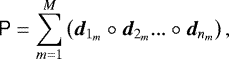
Let s be the sensed phase derivatives in the horizontal and vertical directions, denoted by x and y respectively, projected with the angles θx and θy. We define P as a tensor of N-dimensions and size I1 × I2 × ...IN, where N is the number of layers to be computed. Let dn matrices of size In × M represent the phase derivative at each atmospheric layer N, where M is the decomposition rank of the main tensor P. For simplicity, the following explanation will be made only for the x derivative, but the same reasoning can be followed for the y direction. Also, for convenience, the spatial resolution in every dimension was assumed to be the same due to common phase sensors being symmetric. This decomposition can be written as
 (1)
(1)
where ° represents the outer product of two arrays. In Fig. 1 a schematic representation of the decomposition for a N-dimensional array into its components is depicted. The M value can be seen as a way to decompose the main factorization into a subset of M subproblems. There should be an increase in terms of the quality of the tomography when choosing a higher rank (Wetzstein et al. 2012).
The values of s must be distributed into P according to the cells of each layer that are being traversed by the same light ray. The indexes can be computed as
 (2)
(2)
where hn is the height corresponding to each layer and x0 is the spatial coordinate in the pupil’s plane. Depending on the size of the problem, for example, the number of atmospheric layers, we will get a set of χn ={χ1, χ2, ...χN} in charge of defining the position of every pixel of s within P. According to this, the nonzero values of P are then defined as
 (3)
(3)
This results in P being a sparse matrix (or tensor if N > 2), where only the sampled angles are represented.
Lee & Seung (2001) proposed two gradient descent algorithms to decompose a matrix into factors. The first algorithm consists of an alternating least squares (ALS) minimization of the squared l2-norm
![\begin{equation*} \argmin_{D_{n}} ||\tens{P}-\tens{W}\circledast[\vec{D}_{1}, \vec{D}_{2} \cdots \vec{D}_{N}]||_{2}^{2}, \end{equation*}](/articles/aa/full_html/2018/06/aa32597-18/aa32597-18-eq4.png) (4)
(4)
where Dn is defined as ![$\vec{D}_{n} = [\vec{d}_{n_{1}}, \vec{d}_{n_{2}}, \dots \vec{d}_{n_{m}}]$](/articles/aa/full_html/2018/06/aa32597-18/aa32597-18-eq5.png) . The expression [D1, D2⋯DN] represents a temporary tensor defined by Eq. (1) at each iteration, with every D fixed except the one being minimized. A weighting tensor W has the same size as P. Usually, W is used as a binary sparse tensor where only the nonzero P positions are set as one, although some works have benefited from specific weighting patterns (Chen et al. 2014). A set of multiplicative update rules was derived in Lee & Seung (2001), although different alternatives were also proposed as the Kullback-Leibler divergence. These rules were later expanded to N-dimensions by Morup et al. (2006) and can be defined as
. The expression [D1, D2⋯DN] represents a temporary tensor defined by Eq. (1) at each iteration, with every D fixed except the one being minimized. A weighting tensor W has the same size as P. Usually, W is used as a binary sparse tensor where only the nonzero P positions are set as one, although some works have benefited from specific weighting patterns (Chen et al. 2014). A set of multiplicative update rules was derived in Lee & Seung (2001), although different alternatives were also proposed as the Kullback-Leibler divergence. These rules were later expanded to N-dimensions by Morup et al. (2006) and can be defined as
 (5)
(5)
where P(n) is the matricization or unfolding operation of P along the nth dimension (see lower part of Fig. 1). The ⊛ operator is defined as the element-wise product, and D⊙,(n) is defined by
 (6)
(6)
where ⊙ is the Khatri-Rao product. This product is defined for two matrices  and
and  as
as
![\begin{equation*} \vec{A} \odot \vec{B} = \left[ \begin{array}{cccc} a_{1} \otimes b_{1} & a_{2} \otimes b_{2} & \cdot \cdot \cdot & a_{M} \otimes b_{M} \end{array} \right]. \end{equation*}](/articles/aa/full_html/2018/06/aa32597-18/aa32597-18-eq10.png) (7)
(7)
The Kronecker product is represented as ⊗ and is defined for two matrices  and
and  as a matrix
![\begin{equation*} C \otimes D = \left[ \begin{array}{cccc} c_{11}D & c_{12}D & \cdots & c_{1J}D \\ c_{21}D & c_{22}D & \cdots & c_{2J}D \\ \vdots & \vdots & \ddots & \vdots \\ c_{I1}D & c_{I2}D & \cdots & c_{IJ}D \end{array} \right]. \end{equation*}](/articles/aa/full_html/2018/06/aa32597-18/aa32597-18-eq14.png) (8)
(8)
This can be seen as building a new matrix of the size of C where every element cij is now substituted by the product of its value by the whole matrix D.
Particularizing Eq. (5) to the atmospheric reconstruction case yields the next expressions
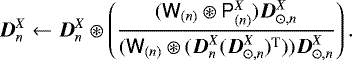 (9)
(9)
The pixels forming  must be rearranged from a two-dimensional phase image to column vectors. The M dimension represents how information from P is distributed into
  . For instance, an N-dimensional rank-1 decomposition will yield N-column vectors, which will contain a compressed form of the data extracted from P (Kolda & Bader 2009; Wang & Zhang 2013). For M = 1, the final partial derivative of the phase will be in the Dn vectors. However, when M > 1, to recover the information it is mandatory to sum all the columns for each Dn along M to obtain the derivative of each phase. This can be expressed as
 (10)
(10)
To obtain the final results in both cases, the column vectors obtained must be rearranged as two-dimensional matrices of size equal to the original sample size of the phase projection for each reference star.
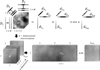 |
Fig. 1 Decomposition of a three-way array into three components of rank M in the weighted nonnegative tensor factorization method. As in Eq. (1), in this example, the product of d1, d2, and d3 must first be computed and then summed along the M-dimension. The matricization operation of tensor P is also depicted in the lower part of the image |
2.2 Randomized Kaczmarz-based method
The Kaczmarz algorithm tries to solve inverse problems by minimizing the residual squared error. As in the previous case, in the following werepresent only one of the two gradients, but the same reasoning can be followed for the other one. Equation (11), previously described in Tallon & Foy (1990), is
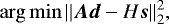 (11)
(11)
where A is a geometric projection matrix for the light rays propagating through the atmosphere, s contains a vectorized form of the previously described phase derivatives vector for each angle in the entrance pupil of the telescope, H is the laser guide star (LGS) projection height, and d contains the variables. In this case, every dn is contained inside the d vector and represents the phase derivative in each direction. In the traditional problem there is no rank-M decomposition of the problem, so every sn is arranged as an Ix1 vector.
A randomized Kaczmarz-based method consists of sweeping randomly the rows of A with a probability proportional to the square of its Euclidean norm to increase the rate of convergence of the algorithm. Strohmer & Vershynin (2009) proposed this method based on previous randomized versions (Herman & Meyer 1993; Frieze et al. 1998; Natterer 2001). Particularizing to this definition yields the next expression
 (12)
(12)
where k is the iteration number, and Ar(i,:) is a random row from matrix A. In this expression, projecting si into the hyperplane ⟨Ar(i,:), dk⟩ gives a certain ratio of convergence according to the conditions presented in the aforementioned work.
2.3 Atmospheric turbulence modeling
We based our simulations on an atmosphere model calculated for the emplacement of Gemini South telescope at La Serena, Chile (Cortes et al. 2012). This model is composed of seven turbulent layers with a global Fried parameter of 15.4 cm, a resolution of 256 × 256 pixels; the model’s turbulence profile ( ) and altitudeare summarized in Table 1. This profile has shown realistic results in previous works (Trujillo-Sevilla 2017). Each layer was simulated independently according to its corresponding
  value, assuming that it follows a Kolmogorov spectrum (Kolmogorov 1941) and the Lane et al. (1992) approximation that involves the addition of subharmonics to the phase screen.
Atmospheric model specifications.
2.4 Simulations
A total of 1000 independent atmospheres were simulated following the above methodology and recovered by both explained methods. In each case, atmospheric turbulence was recovered in two and three layers. Layer heights were set to be recovered at 0 and 4 500 m for two layers, and 0, 4 500 m, and 9 000 m for three layers. In both cases, four different LGS constellations were simulated with a subtended angle of 96.68 arcsec: triangle shaped with and without an on-axis star (Figs. 2b and 2a respectively), and square shaped with and without an on-axis star (Figs. 2d and 2c respectively). The LGSs were considered to be punctual and placed at a height of 90 km in order to simplify the model. A telescope with an 8 m pupil diameter was simulated. Starting from the initial field produced by each LGS, successive propagations of the field through each layer and the telescope itself provided a corresponding image at the focal plane of the telescope for each oneof the references. We assumed that from each punctual LGS, the cone of light that is propagated to the pupil plane of the telescope is perfectly detected by an ideal wavefront phase sensor with a resolution of 32 × 32 pixels. Also, a perfect deformable mirror was considered for the correction of the atmosphere. Final phase reaching a noiseless theoretical sensor was calculated by subtracting the recovered phase from the original atmospheric turbulence. Then, the two-dimensional Strehl ratio across the FoV of the telescope was calculated for each simulated atmosphere. An average of the totality of images was calculated and the radial average of the Strehl ratio from center to off-axis angles were used as a merit function in order to estimate the quality of phase reconstruction for both methods. Variance calculation was also performed. An additional analysis was performed in order to test the behavior of both methods in nondefined layer heights. In this analysis, atmosphericlayers were set to be recovered at 1000, 3000, and 8000 m, using the square shaped on-axis LGS (2d) constellation. The rest of the simulation for this special analysis followed the same methodology described above.
To place the obtained results in context, a threshold for the maximum Strehl ratio that can be obtained assuming a perfect process of measurement and correction of the phase can be derived for the defined system by following the Maréchal approximation (Maréchal 1948) defined as
 (13)
(13)
where μ ranges from 0.2 and 1 depending on the influence of each of the deformable mirror actuators (Roddier 1999). Substituting L as the number of subapertures in the sensor, and D as the pupil’s diameter, yields a theoretical upper limit for the Strehl ratio of 0.6386. To compare the estimated values with our implementation, we ran a set of 1000 simulations in which each atmospheric layer was perfectly corrected since the original values are known. This simulation revealed a constant mean value of 0.6361 throughout the FoV with a standard deviation of 0.0414, very close to the expected value using Eq. (14) (S = 0.6386).
2.5 Algorithm implementation
The randomized Kaczmarz and the WNTF solvers were implemented on MatlabR2016a (Matworks, Natick, MA). The number of iterations on the Kaczmarz method was set at 20 due to previous trials showing almost no improvement in the Strehl ratio after this number. The WNTF solver was built over the Bader & Kolda (2007) Tensor Toolbox. It was set to decompose P (see Eq. (1)) into two and three matrices in relation to the different number of atmospheric layers to be recovered. The number of iterations was set to 100 according to previous tests. The decomposition rank was set to 32 to compare results between both methods and to match the resolution of the simulated wavefront phase sensor, granting a Hadamard product of the objective matrices. Calculationsmade with WNTF required an initial solution. Every atmospheric layer was initialized to Gaussian noise with mean μ = 0 and standard deviation σ = 1 and then the results were normalized between 0 and 1. Although it has been previously demonstrated in the bibliography that initializing the matricesDn in this way can be very inefficient (Langville et al. 2006; Kolda & Bader 2009; Carmona-Ballester et al. 2017), the estimation of a proper initialization method could show itself as a complex problem. For the sake of clarity, this work will not assess these initialization techniques. Nevertheless, better results would be achieved if this was the case.
2.6 Statistical analysis
To properly validate the statistical significance of the obtained radially-averaged Strehl ratios, a t-test hypothesis contrast was carried across the FoV (from 0 to 48.34 arcsec in 0.77 arcsec steps) between different combinations of methods, number of layers, and LGS constellations. A p-value ≤ 0.05 was considered statistically significant.
3 Results
Figure 3 shows an example of a two-dimensional Strehl ratio for the square shaped (on-axis) LGS constellation (see 2d) when averaging 1000 simulated atmospheres. In this case, the WNTF method provided the highest Strehl ratio and a lesser decrease of its value across the FoV of the telescope once atmospheric turbulence was corrected.
The resulting radially-averaged Strehl ratio is shown in Fig. 4 for each method, LGS constellation, and numberof layers. In these cases, the height of the recovered layers is coincident with the height of the defined layers. The discontinuous line represents the radially-averaged Strehl ratio of the telescope without any correction. The variance is also represented for eight equally spaced cases from 0 to 48.34 arcsec. Every WNTF reconstruction provided better Strehl ratio values along the curve than any of the Kaczmarz algorithm configuration (p ≤ 0.05). Also, the radially-averaged Strehl ratio obtained when computing the reconstruction for nondefined layers’ height, at 1000, 3000, and 8000 m, is shown in Fig. 5 for the square shaped (on-axis) LGS constellation (see Fig. 2d). The reconstruction suffered from a general reduction in Strehl value across all the FOV in both methods. The difference in Strehl ratio between both methods has also been reduced, although the WNTF had an overall better Strehl value than the Kaczmarz method (p ≤ 0.05). Variance stayed approximately equal in both situations.
Intra-method differences (i.e., the differences between results for the same method but different number of layers and/or LGS constellation) were also analyzed. The Kaczmarz method showed the best result when performing a three layer reconstruction using the square shaped (on-axis) LGS constellation. The WNTF method provided a better Strehl ratio in every three layer case when compared to the two layer configuration (p ≤ 0.05). This was not the case when comparing for each LGS constellation. The statistical analysis between every WNTF case is summarized in Fig. A.1.
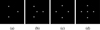 |
Fig. 2 Different laser guide stars (LGS) constellations employed in the simulations. From left to right, (a) triangle shaped, (b) triangle shaped with on-axis LGS, (c) square shaped, (d) and square shaped with on-axis LGS. Each square side represents a sky coverage of 97.8 arcsec. |
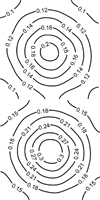 |
Fig. 3 Radially-averaged Strehl ratio across the field of view of a 8m diameter telescope after 1000 simulations for (upper) Kaczmarz and (lower) WNTF methods. The conditions of the simulations comprised three atmospheric layers, 96.68 arcsecof sky coverage and, as laser guiding stars (LGS) configuration, a square shaped with on-axis LGS. |
4 Summary and conclusions
In this paper the WNTF method was tested as a potential technique to be applied in AT based on the promising results obtained in glasses-free three-dimensional displays. The novelty of this approach is to understand data from WFSs as a lightfield. Our results suggest that the WNTF method is a very promising technique in the three-dimensional reconstruction of atmosphere turbulence. It is worth noting that WNTF is a method in which the obtained results are highly influenced by the initial approximation of the objective matrices (Langville et al. 2006; Kolda & Bader 2009; Wang & Zhang 2013; Carmona-Ballester et al. 2017). In this study we have used a common approximation to the initial guess, which consists of setting the matrices with Gaussian noise. According to the aforementioned citations, even though results have exceeded the ones obtained with a more traditional method, we can hypothesize that a tailored initialization would bring even better reconstructions.
To compare these results, a random Kaczmarz-based method was implemented (Strohmer & Vershynin 2009). Despite the existence of a wide variety of different algorithms for AT reconstruction (Saxenhuber et al. 2017), the Kaczmarz method is one of the most explored in the bibliography when dealing with the AT problem and could be considered as a good starting point for comparisons (Ramlau et al. 2014; Auzinger 2015; Auzinger et al. 2015).
The Strehl ratio across the FoV was used in this work as a means to evaluate the quality of the reconstruction. These values should be taken as a qualitative evaluation of the goodness of the proposed approach, as they represent the outcomes of a system composed of an atmosphere defined by only 256 × 256 pixels. This serves to simplify calculations and such an approximation is not uncommon in the scientific bibliography, but it prevents us from knowing the final quantitative scope of the improvement in a real situation (Rigaud et al. 2016). A reference Strehl value was estimated in Sect. 2.4 as a mean to give a context to the obtained results.
The randomized Kaczmarz algorithm was outperformed by WNTF in every case (p ≤ 0.05). Remarkably, the WNTF method also yielded better results in its two layer configurations than the Kaczmarz method for the three layer tomography. In general, WNTF with three layers provided better results than WNTF with two layers. As seen in previous works, a better reconstruction should be obtained when the number of layers is increased. (Wetzstein et al. 2012; Saxenhuber et al. 2017). Also, it was shown that when computing atmospheric layers at different heights than the ones defined by our system, WNTF stayed as the best alternative.
As stated in Sect. 2.1, the minimization problem of WNTF is based on the ALS algorithm. However, the minimization is carried out by alternating which terms are fixed while the tensor P is being decomposed. There are some discrepancies in the literature as to the convergence of this algorithm. For example, Lee & Seung (2001) stated that the multiplicative update rules granted a convergence to a local minimum whenever the matrix was nonnegative, though at a slow rate. However, Wang & Zhang (2013) concluded that the stationary point reached by this method might not always be a local minimum when inside of the feasible region. Comparing this to the randomized Kaczmarz method where the minimization of the l2 − norm is carried as a whole leads us to conclude that the results in the last method might be always superior in terms of the error. In light of the obtained results, where WNTF improves the Kaczmarz tomography, a deeper analysis between both methods should be carried out to clarify this behavior.
Different LGS constellations were employed in simulations in order to know if the obtained improvement was dependent on the LGS constellation. The results showed that WNTF was superior in all cases. Although analysis of the intra-method influence of LGS constellation topology was not the central topic of this work, reconstructions for each configuration in the WNTF method showed a very similar result, though strong statistical evidence was not found. Nevertheless, a tendency for improvement when the total number of LGSs was increased and/or a central star was located in the middle of the constellation was present in the simulations (see Appendix A). This tendency is in agreement with the bibliography for other methods, where it has been stated that a higher number of LGS would be required when trying to decompose the atmosphere into more for the system not to be excessively ill-posed (Saxenhuber et al. 2017).
In order to use these methods in real telescopes, the AT problem should be solved in real-time. Both tested algorithms were implemented on an off-line solver, and therefore, the computational cost of such decompositions would need a specific adaptation of such algorithms, that is, would need parallel computing. Vavasis (2010) stated that the complexity for the classic NMF algorithm of applying multiplicative update rules is of nondeterministic polynomial time (NP-hard). This is especially important in the WNTF method, where an increase in the dimensionality of P would cause a massive increase in the objective matrices’ size during intermediate steps of the multiplicative update rules (Morup et al. 2006). In this work we have focused on the theoretical applicability of the method, postponing the possibilities of real time implementation. This is the reason for our choice of two and three layer configurations. Nevertheless, it has been previously shown that the WNTF method for two layers (Elble et al. 2010) is likely to be implemented in parallel computation (Mejía-Roa et al. 2015). We might speculate that a parallelized version of this algorithm with a higher number of layers could be also implemented although we did not test it.
This work has several limitations and should be taken as a proof of concept. The simulations of the atmosphere patterns, ideal punctual LGS, the capture stage, and the correction procedure were so idealized that only a qualitative difference for the proposed algorithm could be achieved. Nonetheless, a more precise simulation like the one proposed in Andersen et al. (2012) could give a deeper insight into this new technique. However, a consistent qualitative improvement of the WNTF method with respect to a proved methodology like the randomized Kaczmarz method was presented, which underlines the possibilities of this technique that has not yet been studied in the field of atmospheric tomography.
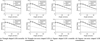 |
Fig. 4 Radially-averaged Strehl ratios across the field of view of an 8 m diameter telescope, obtained by the average of 1000 simulations when applying both methods in four LGS constellations. The variance of some equally-spaced points are represented alongside. The first row shows the results for a decomposition of two layers, and second row shows the results for three layers. The line labeled as reference represents the Strehl ratio of the telescope without any correction. The maximum possible Strehl ratio for this simulation is 0.6386 across all the FoV (see Eq. (14)). In order to keep clarity, this value has not been included in the graphs |
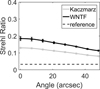 |
Fig. 5 Performance in terms of radially-averaged Strehl ratio across the field of view when recovering three atmospheric layers at heights different from the defined heights (1000, 3000 and 8000 m). The LGS constellation used was the square shaped on-axis. |
Acknowledgements
We want to thank the valuable support of the CAFADIS group of the University of La Laguna (Tenerife, Spain). We would also like to thank our reviewers for their valuable advice. This work was supported by the Spanish Ministry of Economy under the project DPI2015-66458-C2-2-R and by ERDF funds from the European Commission.
Appendix A Statistical analysis for the WNTF case in the three layer configuration
 |
Fig. A.1 Statistical relation between the intra methods presented in Sect. 3. Each square color represents which configuration is the best between tested layer and LGS configurations and from which point of the curve the difference is statistically significant. A gray square means no difference was found. |
References
- Andersen, D. R., Jackson, K. J., Blain, C., et al. 2012, PASP, 124, 469 [NASA ADS] [CrossRef] [Google Scholar]
- Anderson, J. M., Mair, B. A., Rao, M., & Wu, C. H. 1997, IEEE Trans. Med. Imaging, 16, 159 [CrossRef] [Google Scholar]
- Auzinger, G. 2015, in On choosing layer profiles in atmospheric tomography, J. Phys. Conf. Ser., 595, 012001 [CrossRef] [Google Scholar]
- Auzinger, G., Le Louarn, M., Obereder, A., & Saxenhuber, D. 2015, in Adaptive Optics for Extremely Large Telescopes IV, Conf. Proc., E2 [Google Scholar]
- Bader, B. W., & Kolda, T. G. 2007, SIAM J. Sci. Comput., 30, 205 [CrossRef] [Google Scholar]
- Beckmann, E. C. 2006, Br. J. Radiol., 79, 5 [CrossRef] [Google Scholar]
- Carmona-Ballester, D., Trujillo-Sevilla, J. M., Bonaque-González, S., Hernández-Delgado, A., & Rodríguez-Ramos, J. M. 2017, Opt. Eng. 57, 061603 [Google Scholar]
- Chen, R., Maimone, A., Fuchs, H., Raskar, R., & Wetzstein, G. 2014, J. Soc. Inf. Disp., 22, 525 [CrossRef] [Google Scholar]
- Cichocki, A., Zdunek, R., Phan, A. H., & Amari, S. I. 2009, Nonnegative Matrix and Tensor Factorizations: Applications to Exploratory Multi-Way Data Analysis and Blind Source Separation 1st edn. (Hoboken, USA: John Wiley & Sons), 1 [Google Scholar]
- Cormack, A. M. 1964, J. Appl. Phys., 35, 2908 [NASA ADS] [CrossRef] [Google Scholar]
- Cortes, A., Neichel, B., Guesalaga, A., et al. 2012, Proc. SPIE - The International Society for Optical Engineering, 8447, 1 [NASA ADS] [Google Scholar]
- Elble, J. M., Sahinidis, N. V., & Vouzis, P. 2010, Parallel Comput., 36, 215 [CrossRef] [Google Scholar]
- Ellerbroek, B. L. 2002, J. Opt. Soc. Am. A, 19, 1803 [NASA ADS] [CrossRef] [Google Scholar]
- Frieze, A., Kannan, R., & Vempala S., 1998, in Proc. 39th Annual Symp. on Foundations of Computer Science (Cat. No.98CB36280), J. ACM, 51, 370 [Google Scholar]
- Gaarder, N. T., & Herman, G. T. 1972, Comput. Graphics Image Process., 1, 97 [CrossRef] [Google Scholar]
- Gordon, R., Bender, R., & Herman, G. T. 1970, J. Theor. Biol., 29, 471 [CrossRef] [PubMed] [Google Scholar]
- Herman, G. T., & Meyer, L. B. 1993, IEEE Trans. Med. Imaging, 12, 600 [CrossRef] [Google Scholar]
- Hounsfield, G. N. 1973, Br. J. Radiol., 46, 1016 [Google Scholar]
- Kaczmarz, S. 1937, Bull. Int. Acad. Pol. Sci. Lett., 35, 355 [Google Scholar]
- Kolda, T. G., & Bader, B. W. 2009, SIAM Rev., 51, 455 [Google Scholar]
- Kolmogorov, A. 1941, Doklady Akademii Nauk SSSR, 30, 301 [Google Scholar]
- Lane, R. G., Glindemann, A., & Dainty, J. C. 1992, Waves in Random Media, 2, 209 [NASA ADS] [CrossRef] [Google Scholar]
- Langville, A. N., Meyer, C. D., & Albright, R. 2006, in Proceedings of the 12th ACM SIGKDD international conference on Knowledge discovery and data mining, 1 [Google Scholar]
- Le Louarn, M., Hubin, N., Sarazin,M., & Tokovinin, A. 2000, MNRAS, 317, 535 [NASA ADS] [CrossRef] [Google Scholar]
- Lee, D. D., & Seung, H. S. 2001, in Advances in Neural Information Processing Systems 13, Proc. Conf. NIPS 2000, eds. T. K. Leen, T. G. Dietterich & V. Tresp (NIPSC), 556 [Google Scholar]
- Maréchal, A. 1948, Éditions de la Revue d’optique théorique et instrumentale, 21, A2213 [Google Scholar]
- Mejía-Roa, E., Tabas-Madrid, D., Setoain, J., et al. 2015, BMC Bioinf., 16, 43 [CrossRef] [Google Scholar]
- Morup, M., Hansen, L. K., Parnas, J., & Arnfred, S. M. 2006, Informatics and Mathematical Modelling, Technical Report, University of Denmark [Google Scholar]
- Natterer, F. 2001, The Mathematics of Computerized Tomography, Classics in applied mathematics, (Philadelphia: SIAM) 32 [CrossRef] [Google Scholar]
- Paatero, P., & Tapper, U. 1994, Environmetrics, 5, 111 [CrossRef] [Google Scholar]
- Pauca, V., Shahnaz, F. W., Berry, M., & Plemmons, R. 2004, in Proc. of the 4th SIAM international conference on data mining (Lake Buena Vista, Florida, USA: SIAM) [Google Scholar]
- Philip Hart, II V. 2012, PhD Thesis, Utah State University [Google Scholar]
- Ramlau, R., & Rosensteiner, M. 2012, Inverse Prob., 28 [Google Scholar]
- Ramlau, R., Saxenhuber, D., & Yudytskiy, M. 2014, in Proc. SPIE, 9148, 91480Q [CrossRef] [Google Scholar]
- Rigaud, G., Bellet, J. B., Berginc, G., Berechet, I., & Berechet, S. 2016, IEEE Geosci. Remote Sens. Lett., 13, 936 [NASA ADS] [CrossRef] [Google Scholar]
- Roddier, F. 1999, Adaptive Optics in Astronomy (Cambridge, UK: Cambridge University Press), 419 [Google Scholar]
- Saxenhuber, D., Auzinger, G., Louarn, M. L., & Helin, T. 2017, Appl. Opt., 56, 2621 [NASA ADS] [CrossRef] [Google Scholar]
- Strohmer, T., & Vershynin, R. 2009, J. Fourier Anal. Appl., 15, 262 [CrossRef] [Google Scholar]
- Tallon, M., & Foy, R. 1990, A&A, 235, 549 [NASA ADS] [Google Scholar]
- Trujillo-Sevilla, J. 2017, PhD Thesis, Universidad de La Laguna, Spain [Google Scholar]
- Vavasis, S. A. 2010, SIAM J. Optim., 20, 1364 [CrossRef] [Google Scholar]
- Wang, Y.-X., & Zhang, Y.-J. 2013, IEEE Trans. Knowl. Data Eng., 25, 1336 [CrossRef] [Google Scholar]
- Wetzstein, G., Lanman, D., Hirsch, M., & Raskar, R. 2012, ACM Trans. Graph. (Proc. SIGGRAPH), 31, 1 [CrossRef] [Google Scholar]
All Tables
All Figures
|
Fig. 1 Decomposition of a three-way array into three components of rank M in the weighted nonnegative tensor factorization method. As in Eq. (1), in this example, the product of d1, d2, and d3 must first be computed and then summed along the M-dimension. The matricization operation of tensor P is also depicted in the lower part of the image |
| In the text | |
|
Fig. 2 Different laser guide stars (LGS) constellations employed in the simulations. From left to right, (a) triangle shaped, (b) triangle shaped with on-axis LGS, (c) square shaped, (d) and square shaped with on-axis LGS. Each square side represents a sky coverage of 97.8 arcsec. |
| In the text | |
|
Fig. 3 Radially-averaged Strehl ratio across the field of view of a 8m diameter telescope after 1000 simulations for (upper) Kaczmarz and (lower) WNTF methods. The conditions of the simulations comprised three atmospheric layers, 96.68 arcsecof sky coverage and, as laser guiding stars (LGS) configuration, a square shaped with on-axis LGS. |
| In the text | |
|
Fig. 4 Radially-averaged Strehl ratios across the field of view of an 8 m diameter telescope, obtained by the average of 1000 simulations when applying both methods in four LGS constellations. The variance of some equally-spaced points are represented alongside. The first row shows the results for a decomposition of two layers, and second row shows the results for three layers. The line labeled as reference represents the Strehl ratio of the telescope without any correction. The maximum possible Strehl ratio for this simulation is 0.6386 across all the FoV (see Eq. (14)). In order to keep clarity, this value has not been included in the graphs |
| In the text | |
|
Fig. 5 Performance in terms of radially-averaged Strehl ratio across the field of view when recovering three atmospheric layers at heights different from the defined heights (1000, 3000 and 8000 m). The LGS constellation used was the square shaped on-axis. |
| In the text | |
|
Fig. A.1 Statistical relation between the intra methods presented in Sect. 3. Each square color represents which configuration is the best between tested layer and LGS configurations and from which point of the curve the difference is statistically significant. A gray square means no difference was found. |
| In the text | |
Current usage metrics show cumulative count of Article Views (full-text article views including HTML views, PDF and ePub downloads, according to the available data) and Abstracts Views on Vision4Press platform.
Data correspond to usage on the plateform after 2015. The current usage metrics is available 48-96 hours after online publication and is updated daily on week days.
Initial download of the metrics may take a while.