| Issue |
A&A
Volume 614, June 2018
|
|
|---|---|---|
| Article Number | A51 | |
| Number of page(s) | 14 | |
| Section | Astrophysical processes | |
| DOI | https://doi.org/10.1051/0004-6361/201731830 | |
| Published online | 12 June 2018 | |
Radiatively driven relativistic jets in Schwarzschild space-time
1
Aryabhatta Research Institute of Observational Sciences (ARIES),
Manora Peak,
Nainital
263002,
India
e-mail: This email address is being protected from spambots. You need JavaScript enabled to view it.
; This email address is being protected from spambots. You need JavaScript enabled to view it.
2
Departement of Physics and Astrophysics, Delhi University,
New Delhi,
India
Received:
25
August
2017
Accepted:
27
January
2018
Abstract
Context. Aims. We carry out a general relativistic study of radiatively driven conical fluid jets around non-rotating black holes and investigate the effects and significance of radiative acceleration, as well as radiation drag.
Methods. We apply relativistic equations of motion in curved space-time around a Schwarzschild black hole for axis-symmetric one-dimensional jet in steady state, plying through the radiation field of the accretion disc. Radiative moments are computed using information of curved space-time. Slopes of physical variables at the sonic points are found using L’Hôpital’s rule and employing Runge-Kutta’s fourth order method to solve equations of motion. The analysis is carried out using the relativistic equation of state of the jet fluid.
Results. The terminal speed of the jet depends on how much thermal energy is converted into jet momentum and how much radiation momentum is deposited onto the jet. Many classes of jet solutions with single sonic points, multiple sonic points, as well as those having radiation driven internal shocks are obtained. Variation of all flow variables along the jet-axis has been studied. Highly energetic electron-proton jets can be accelerated by intense radiation to terminal Lorentz factors γT ~ 3. Moderate terminal speed vT ~ 0.5 is obtained for moderately luminous discs. Lepton dominated jets may achieve γT ~ 10.
Conclusions. Thermal driving of the jet itself and radiation driving by accretion disc photons produce a wide-ranging jet solutions starting from moderately strong jets to the relativistic ones. Interplay of intensity, the nature of the radiation field, and the energetics of the jet result in a variety of jet solutions. We show that radiation field is able to induce steady shocks in jets, one of the criteria to explain high-energy power-law emission observed in spectra of some of the astrophysical objects.
Key words: hydrodynamics / ISM: jets and outflows / shock waves / black hole physics / radiation mechanisms: general / relativistic processes
© ESO 2018
1 Introduction
While analysing an optical image of M 87, Curtis (1918) made a note of a “curious straight ray... connected with the nucleus” which was later identified and termed a “relativistic jet” (Baade & Minkowski 1954). Since then, the observational study of jets has been revolutionized and these objects established as ubiquitous astrophysical phenomena associated with various classes of other objects like active galactic nuclei (AGN, e.g., M 87), young stellar objects (YSO, e.g., HH 30, HH 34), X-ray binaries (e.g., SS433, Cyg X-3, GRS 1915+105, GRO 1655–40), gamma ray bursts (e.g., GRB 980519), and pulsar wind nebulae (Porth et al. 2017), and so on.
This paper investigates the properties of relativistic jets around black hole (BH) candidates like X-ray binaries and AGNs. In such systems, jets can only emerge from accreting matter, as BHs do not have hard surfaces and are not capable of emission. This fact is supported by strong correlation observed between spectral state of the accretion disc and jet (Gallo et al. 2003; Fender et al. 2010; Rushton et al. 2010). Observations also limit the jet generation region to a distance of less than 100 Schwarzschild radii (rs) around the central object (Junor et al. 1999; Doeleman et al. 2012). This implies that the entire accretion disc does not take part in jet generation.
Ever since the emergence of the first theoretical model of accretion discs, that is, the Keplerian disc (KD; Shakura & Sunyaev 1973), or later disc models like the thick disc (TD; Paczyński & Wiita 1980), the advection-dominated accretion flow (ADAF; Narayan et al. 1997) and advective discs (Fukue 1987; Chakrabarti 1989), there have been many attempts to understand how photons radiated from these discs interact with jets emerging from them. The equations of motion (EoM) of radiation hydrodynamics (RHD) were developed by many authors (Hsieh & Spiegel 1976; Mihalas & Mihalas 1984; Kato et al. 1998) in special relativity (SR). Later the general relativistic (GR) version of those equations was also obtained (Park 2006; Takahashi 2007). Many authors used these EoMs under a variety of approximations to study radiatively driven jets. Icke (1980) studied the matter flow in the radiation field above a Keplerian disc. Sikora & Wilson (1981) studied particle jets in SR regime, driven by the radiation field in the funnel of a thick accretion disc and obtained a terminal speed of vT ~ 0.4c (c ≡ speed of light in vacuum) for electron-proton or e−−p+ jets, although the terminal Lorentz factor obtained was γT ~ 3 for electron-positron or e−− e+ jets. Icke (1989) obtained a theoretical upper limit or “magic speed” vm = 0.45c above a KD using the near disc approximation for radiation field. Any speed above vm would invoke radiative deceleration induced by radiation drag. Around the same time, Ferrari et al. (1985, hereafter FTRT85) studied radiation interaction with a fluid jet in SR regime. They mostly assumed isothermal jets with a non-radial cross-section. A Newtonian gravitational field was added ad hoc to the EoM. The radiation field was computed from disc models for a variety of disc thicknesses. They obtained mildly relativistic jets and shocks induced by the non-radial nature of the jet cross-section, as well as the radiation field. Fukue (1996) studied radiatively driven off-axis particle jets, using the radiation field similar to Icke. The detailed radiation field around a BH was calculated by Hirai & Fukue (2001) above a KD governed by a point mass gravity using Newtonian and pseudo-Newtonian potentials (pNp) to mimic non-rotating and rotating BH exterior. The strength of the radiation field using Schwarzschild pNp was found to be half of the Newtonian potential, but it was about one order greater for Kerr pNp. In another attempt, Fukue et al. (2001) considered a hybrid disc consisting of outer KD and inner ADAF. Such a scenario produced jets with γT ~ 2, and also induced collimation.
It may be noted that a large number of jet studies in recent years have relied on numerical simulations. Most of these works investigate how special relativistic jets interact with the ambient medium, or how magnetic field affects them (Duncan & Hughes 1994; Marti & Muller 1997; Agudo et al. 2001; Komissarov et al. 2007; Mignone et al. 2010). Tchekhovskoy et al. (2011), on the other hand, simulated magnetically arrested disc and jet launching from such a disc. Although not a simulation, Meliani et al. (2006) studied steady jets in the meridional plane in general relativistic magneto hydrodynamics (GRMHD). These kind of studies are important because they enhance the understanding of the system and act as test cases for numerical simulations.
Most of the jet simulations did not include radiatively driven jets. Simulations which did include interaction of radiation with outflows were mainly in the non-relativistic limit (Chattopadhyay & Chakrabarti 2002b; Chattopadhyay et al. 2012). There is a general consensus that radiation cannot accelerate fluid jets to relativistic speeds (Guthmann et al. 2002), and that is probably the reason why simulations of radiatively driven jets are few in number. General relativistic simulations which include the interaction of radiation with matter exist, but they study either the stellar collapse scenario (Farris et al. 2008), or Bondi-Hoyle accretion (Zanotti et al. 2011) and that too in optically thick medium while jets are divergent flows and are optically thin.
In the advective disc regime, numerical simulations (Molteni et al. 1996; Das et al. 2014; Lee et al. 2016) and theoretical investigations (Chattopadhyay & Das 2007; Kumar & Chattopadhyay 2013, 2017; Kumar et al. 2014, 2013; Chattopadhyay & Kumar 2016) showed that the extra-thermal gradient force in the post-shock region automatically generates bipolar outflows. Anticipating that the intense radiation from the accretion disc may accelerate jets, Chattopadhyay & Chakrabarti (2000a,b, 2002a,b) investigated radiative driving of jets by advective disc photons. It was noted that cold jets could be efficiently accelerated to vT ~ few × 0.1c. But to achieve vT > 0.9c for jets, the required base temperature and injection speed was quite high, which does not match with inner accretion disc parameters. Moreover, being in the non relativistic regime, the formalism followed by Chattopadhyay & Chakrabarti (2000a, 2002a) is only correct up to the first order of the flow velocity. In order to gauge the full extent of radiative acceleration, investigations of radiatively driven particle jets in SR regime (Chattopadhyay et al. 2004; Chattopadhyay 2005) were undertaken. Under such conditions, disc photons could accelerate jets up to γT >~ 2 and significant collimation could be achieved. The radiation field above such discs has two sources, one being the hard radiation from the inner post-shock disc, and the other being the soft radiation from the pre-shock disc. It may be noted that a compact, hot, low-angular-momentum corona close to the BH, which produces hard radiation, and an external disc producing softer radiation, are not exclusive to shocked advective discs but are seen in many other models (Shapiro et al. 1976; Dove et al. 1997; Gierlinski et al. 1997). Therefore, the source of radiation, that is, the underlying accretion disc, may be an advective disc, or any other disc model which considers a compact, geometrically thick corona close to the BH and an outer disc.
In most of the investigations of relativistic fluid jets, the cross-section was assumed to be spherical (∝ r2, r being the radial distance). Meliani et al. (2004) considered thermally driven relativistic jets in Schwarzschild metric, modifying an approximate equation of state (EoS) of single species relativistic gas (Mathews 1971). They hid the actual acceleration process in an adhoc adiabatic index (Γ) and obtained monotonic jets from mildly- to ultra-relativistic jet terminal speed. In contrast, FTRT85 studied jet driven by radiation, as well as the cross-section deviating from the spherical description. Since then, the possibility of internal shocks in outflows, except for non-spherical solar winds (Leer & Holzer 1990), has rarely been reported; leaving it unclear whether non-conical geometry or the external radiation field triggered the shock in the jet. Vyas et al. (2015, hereafter VKMC15) addressed the problem of radiatively driven fluid jets in SR regime similar to FTRT85, but unlike them, used a relativistic EoS for the fluid and a conical jet geometry. Although VKMC15 produced relativistic vT, no multiple sonic point or shock in jets was obtained. We focussed on the role of jet geometry in Vyas & Chattopadhyay (2017, hereafter VC17) and compared thermally driven relativistic jets with a spherical cross-section to those with a non-spherical one. We showed, jets with non-spherical cross-section indeed produce multiple sonic points and shock. However, there was no shock for flows with conical jets.
In this paper, we revisit the problem as posed by FTRT85 and Meliani et al. (2004), that is, we consider radiatively driven jets, like the former authors, but for conical jets, like the latter, such that no shock can form due to the flow geometry of the jet. We use a relativistic EoS for a multispecies gas and solve the jet EoMs in curved geometry of Schwarzschild metric. One of the main reasons for using Schwarzschild metric instead of pseudo-Newtonian potential (pNp) in special relativistic metric is because the curvature effect on the radiation field is important and affects at least up to a few tens of gravitational radii and also because the pNp makes the flow much hotter than real flows. Moreover, the radiative moments were re-computed from a thicker disc in the curved space-time, complete with all the transformations required to do so. It would be intriguing to study all possible jet solutions as the jet plies through the intense radiation field of the accretion disc. Can radiation accelerate jets to relativistic terminal speeds, starting with reasonable base temperature and speed? Can accretion disc radiation drive a jet shock? In this paper we would like to investigate these questions.
In following section, we present the governing equations and underlying assumptions. We also present the method to compute radiative moments from the approximate accretion solutions and outline the solution methodology. We then present the results in Sect. 3. In Sect. 4 we conclude the paper discussing the outcomes and significance.
2 Assumptions and governing equations
2.1 Assumptions
The space-time around a non-rotating black hole is described by Schwarzschild metric:
 (1)
(1)
Here r, θ, and ϕ are usual spherical coordinates, t is time, gμμ are diagonal metric components,MB is the mass of the central black hole and G is the universal constant of gravitation. Hereafter, we use geometric units (unless specified otherwise) where G = MB = c = 1, such that the units of mass, length, and time are MB, rg = GMB∕c2, and tg = GMB∕c3, respectively.In this system of units, the event horizon or Schwarzschild radius is at rs = 2. The jet is assumed to be in steady state (i.e. ∂∕∂t = 0). A jet cannothave high angular momentum, otherwise it will not remain collimated. Moreover, efficient removal of jet angular momentum by the radiation has also been reported before (Fukue et al. 2001; Chattopadhyay 2005); therefore, for simplicity we assume jets to be non-rotating(uϕ = 0), on-axis (i.e. uθ = 0) and axis-symmetric (∂∕∂ϕ = 0) with a small opening angle. Narrow jet allows us to further assume that at distance r, the physical variables of the jet remain the same along the transverse direction. In this study, the jet is assumed to expand radially along the rotation axis of the accretion disc.
The source of radiation is the accretion disc. The dominant radiative cooling processes considered in the disc are synchrotron, bremsstrahlung, and, in addition, inverse-Comptonization in the corona. The magnetic pressure in the accretion disc is assumed to be due to stochastic magnetic field. The ratio of the gas pressure to the magnetic pressure is given by β. We take β = 2.0 in this paper. The cooling process in the corona is implemented through a fitting function (VKMC15). This is an exploratory study of astrophysical fluid jets, which are powered by both the thermal gradient term and radiation driving. The accretion disc plays an auxiliary role, that is, it influences the jet only through radiation. The jet is assumed to be fully ionized and the interaction between radiation and matter is dominated by Thomson scattering. Full relativistic transformations are implemented on the radiation field. We use the methods laid down by Beloborodov (2002) and Bini et al. (2015) to incorporate the effect of photon bending in computing radiative moments.
2.2 Governing equations
2.2.1 Equation of state
EoS is the relation between the thermodynamic quantities of fluid, that is, internal energy density (e), pressure (p), and mass density (ρ); it is basically a closure relation between the thermodynamic variables that allows us to solve the equations of motion of a fluid. In this study, we consider EoS for multispecies relativistic flow proposed by Chattopadhyay (2008), Chattopadhyay & Ryu (2009), which is an extremely close approximation of the exact one (Chandrasekhar 1938; Synge 1957). The EoS is given as,
 (2)
(2)
in physical dimensions, where  is the electron number density, me is the electron rest mass and the dimensionless quantity f is given by
![Mathematical equation: \begin{equation*} f=(2-\xi)\left[1+\mathrm{\Theta}\left(\frac{9\mathrm{\Theta}+3}{3\mathrm{\Theta}+2}\right)\right] +\xi\left[\frac{1}{\eta}+\mathrm{\Theta}\left(\frac{9\mathrm{\Theta}+3/\eta}{3\mathrm{\Theta}+2/\eta} \right)\right].\end{equation*}](/articles/aa/full_html/2018/06/aa31830-17/aa31830-17-eq4.png) (3)
(3)
Here, Θ = kT∕(mec2) is a measure of temperature (T), k is Boltzmann constant and 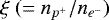 is the relative proportion of number densities of protons and electrons.
 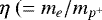 ) is the mass ratio of electrons and protons. The expressions of the polytropic index N, adiabatic index Γ, adiabatic sound speed a, and enthalpy h (in geometric units) are given by
 (4)
(4)
Here τ (= 2 − ξ + ξ∕η) is a function of composition.
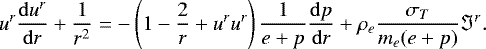
2.2.2 Jet EoM
Equations of motion, that is EoM of radiation hydrodynamics in curved space-time, were derived before (Park 2006; Takahashi 2007), and in the following, we present them in brief. The energy-momentum tensor for matter ( ) and radiation (
 ) are given by
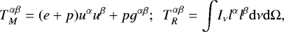 (5)
(5)
where uα are the components of four-velocity, lαs are the directional derivatives, Iν is the specific intensity of the radiation field, where ν is the frequency of the radiation, and dΩ is the differential solid angle subtended by a source point at the accretion disc surface on to the field point at the jet axis.
The ith component of the momentum balance equation is obtained by projecting  with the tensor
  and in steady state it becomes
 (6)
(6)
Here, ρe is total lepton density and ℑr is the net radiative contribution1 and is given by
![Mathematical equation: \begin{equation*} {\mathrm{\Im}}^r=\sqrt{g^{rr}}\gamma^3\left[(1+v^2){\cal R}_1-v \left(g^{rr} {\cal R}_0+\frac{{\cal R}_2}{g^{rr}}\right)\right].\end{equation*}](/articles/aa/full_html/2018/06/aa31830-17/aa31830-17-eq14.png) (7)
(7)
Three-velocity v of the jet is defined as v2 = −uiui∕utut = − ur ur∕utut, that is,  , and γ2 = −utut is the Lorentz factor.
  and
and  are zeroth, first, and second moments of specific intensity of the radiation and can be physically identified as the radiation energy density, the flux, and the pressure, respectively.
In scattering regime, the first law of thermodynamics, or energy equation ( ) is given by,
 (8)
(8)
Therefore, the system is isentropic (Mihalas & Mihalas 1984). Integrating the conservation of mass flux equation (![Mathematical equation: $[\rho u^{\alpha}]_{;\alpha}=0$](/articles/aa/full_html/2018/06/aa31830-17/aa31830-17-eq20.png) ), we obtain the mass outflow rate
), we obtain the mass outflow rate
 (9)
(9)
where  is the cross-section of the jet.
Since the right-hand side of Eq. (8) is zero, then integrating it with the help of the EoS (Eq. (2)) we obtain an adiabatic relation between Θ and ρ (Kumar et al. 2013). Replacing ρ of the adiabatic relation in Eq. (9), we obtain an expression of entropy-outflow rate
 (10)
(10)
where k1 = 3(2 − ξ)∕4, k2 = 3ξ∕4, and k3 = (f − τ)∕(2Θ). This is also a measure of entropy of the jet and in the present context, it remains constant along the jet except at the shock. We integrate Eqs. (6) and (8), and obtain the generalized relativistic Bernoulli parameter in the radiation-driven regime, which is given by E = −hutexp(−Xf), where,
![Mathematical equation: \begin{equation*} X_f=\left(\int \mathrm{d}r \frac{\gamma (2-\xi)}{(f+2 \mathrm{\Theta} )\sqrt{g^{rr}}}\left[(1+v^2){R_1}-v \left(g^{rr} R_0+\frac{R_2}{g^{rr}}\right)\right]\right).\end{equation*}](/articles/aa/full_html/2018/06/aa31830-17/aa31830-17-eq23.png) (11)
(11)
Here,  and
and  are terms proportionalto the radiative moments such as radiation energy density, flux, and pressure, but for simplicity in the rest of the paper, we call these quantities (R0, R1, & R2) as respective radiative moments. The kinetic power of a jet is defined as the energy flux at large distances and is given by
 (12)
(12)
where ![Mathematical equation: $ E_{\infty}=[-hu_t]_{r\rightarrow \infty}$](/articles/aa/full_html/2018/06/aa31830-17/aa31830-17-eq27.png) is the Bernoulli parameter at infinity.
is the Bernoulli parameter at infinity.
Expressing ℘r = σTℑr∕(me), Eqs. (6) and (8) can be expressed as gradients of v and Θ and are given by
 (13)
(13)
and
![Mathematical equation: \begin{equation*} \frac{\mathrm{d}\mathrm{\Theta}}{\mathrm{d}r}=-\frac{{\Theta}}{N}\left[ \frac{{\gamma} ^2}{v}\left(\frac{\mathrm{d}v}{\mathrm{d}r}\right)+\frac{2r-3}{r(r-2)} \right].\end{equation*}](/articles/aa/full_html/2018/06/aa31830-17/aa31830-17-eq29.png) (14)
(14)
Equations (13) and (14) are integrated to solve for v and Θ of a steady jet plying through the radiation field (ℑr) of the underlying accretion disc.
The last term on the right-hand side of Eq. (13) is the radiation momentum deposition term,
 (15)
(15)
with
![Mathematical equation: \begin{equation*} \wp^r=\sqrt{g^{rr}}\gamma^3\left[(1+v^2){R_1}-v \left(g^{rr} R_0+\frac{R_2}{g^{rr}}\right)\right]. \nonumber \end{equation*}](/articles/aa/full_html/2018/06/aa31830-17/aa31830-17-eq31.png)
Equation (15) shows that because of the presence of enthalpy in the denominator, the radiation driving of the jet is more effective for colder jets. The presence of the metric term grr in Rd implies that gravity also affects radiation driving. One can reduce Eq. (15) to non-relativistic limits, if grr → 1, γ2 → 1 and h → 1, then  reduces to (also see, Chattopadhyay & Chakrabarti 2002a; Kumar et al. 2014),
![Mathematical equation: \begin{equation*} {\cal F}_{\textrm{rd}} {\textrm{(NR)}}=\frac{r^2(2-\xi)}{\tau}[{R_1}-v(R_0+R_2)]. \end{equation*}](/articles/aa/full_html/2018/06/aa31830-17/aa31830-17-eq33.png) (16)
(16)
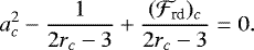
Clearly,  is less interesting, since it is more dependent on the moments and weakly on v. Since the grr term has appeared in Rd, closer to the horizon the third of the term in Eq. (15) dominates. That is, as r →2,
  , therefore, the outward (v > 0) moving jet will decelerate – an effect that cannot be realised even with the special relativistic version of
  (VKMC15). An interesting comparison of equations of motion with Paczyński-Wiita potential and general relativistic analysis is discussed in Appendix B, where we show how pNp is insufficient for relativistic outflows and leads to deviation even at larger distances from BH. The impact of curved space on radiation field and the radiative term is discussed separately in Sect. 3.1. The resultant differences make general relativistic study inevitable for precise study of relativistic dynamics of jets.
Within the funnel for a geometrically thick corona, R1 < 0 as is shown below, and therefore, within the funnel  for outward moving jet, that is, v > 0. But even in regions where R1 > 0,
  , for any v ≥ veq, where,
 (17)
(17)
It is clear from Eq. (17) that the effect of radiation drag is effective in optically thin medium (radiation penetrates the medium) and for distributed source. The negative terms in  depend on v and hence it is termed as “drag term”. One may compare the GR version of veq with the special relativistic and Newtonian versions (Chattopadhyay & Chakrabarti 2002a; Chattopadhyay et al. 2004).
2.3 Radiative moments
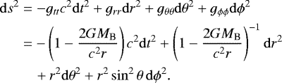
In Fig. 1, we present the schematic diagram of the accretion disc-jet system, where the jet, the corona, and the outer disc are shown. The outer boundary of the corona is xsh, the half height is Hsh, the outer boundary of the outer disc is x0, and the half height is H0. As stated before, the accretion disc plays an auxiliary role in this paper, where it is considered only as a source of radiation. The accretion disc assumed has a geometrically thick, compact corona, which supplies the hard photons by inverse-Comptonization of seed photons, and an outer disc supplying softer photons. Such a disc structure is broadly consistent with many accretion disc models, as been mentioned in Sect. 1. The Keplerian component in the outer disc is ignored because the radiative moments computed from an outer Keplerian disc are negligibly small compared to those from the inner corona, or from the outer advective flow (Chattopadhyay et al. 2004; Chattopadhyay 2005; VKMC15).
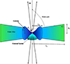 |
Fig. 1 Cartoon diagram of cross-sections of axis-symmetric accretion disc and the associated jet in (r, θ, ϕ coordinates). The shock location xsh, the interceptof outer disc on the jet axis (d0), height of the shock Hsh, and the outer edge of the disc x0 are marked. The semi-vertical angle of the corona is θC and for the outer disc is θD. The funnel of the corona is also shown. |
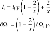
2.3.1 Relativistic transformation of intensities from various disc components
To solve equations of motion of the jet, we need to compute radiative moments on the jet axis, which requires information of specific intensities from both the outer disc and the corona. The details of estimating the temperature (Eq. (A.2)) and velocity(Eq. (A.1)) from accretion discs, and thereby estimating the radiative intensity (Eqs. (A.4), (A.8)), is presented in Appendix A. However, the form of the intensities is in the local rest-frame of the disc surface, and therefore, those intensities need to be transformed from the disc rest frame to the curved frame. After special and general relativistic transformations, the specific intensities become,
![Mathematical equation: \begin{equation*} I_{\textrm{i}}=\frac{{\tilde I}_{\textrm{i}}}{\gamma^4_{\textrm{i}}\left[1+{\vartheta}_jl^j\right]^4_{\textrm{i}}}\left(1-\frac{2}{x}\right)^2,\end{equation*}](/articles/aa/full_html/2018/06/aa31830-17/aa31830-17-eq41.png) (18)
(18)
where Ĩi is the frequency integrated specific intensity measured in the local rest frame of the accretion disc, ϑj is jth component of three-velocity of accreting matter, ljs are directional cosines, γi is the Lorentz factor and x is the radial coordinate of the source point on the accretion disc. The suffix i → C and D signifies the contribution from the corona and the outer disc, respectively. The presense of  in the above equation reduces the intensity of radiation close to the horizon (Beloborodov 2002).
2.3.2 Calculation of radiative moments in curved spacetime
Radiative moments are defined as zeroth, first, and second moments of specific intensity, that is, ∫ IdΩ; ∫ IljdΩ; and ∫ IljlkdΩ, respectively, which are ten independent components (Mihalas & Mihalas 1984; Chattopadhyay 2005). However, it was also found that for a conical narrow jet only three of the moments are dynamically important. If lF is the relevant direction cosine in the flat space-time, then it is related to the one in the curved space as (Beloborodov 2002),
 (19)
(19)
Here, as before i →C and D signifies the contribution from the corona and the outer disc, respectively.
The expressions of flat space differential solid angle dΩi F and direction cosines li F are obtained as:
![Mathematical equation: \begin{equation*} \mathrm{d}\mathrm{\Omega}_{\textrm{i \small F}}=\frac{rx\mathrm{d}\phi \mathrm{d}x}{[(r-x \cos\theta_{\textrm{i}})^2+x^2\sin\theta_{\textrm{i}}^2]^{3/2}}, \end{equation*}](/articles/aa/full_html/2018/06/aa31830-17/aa31830-17-eq44.png) (20)
(20)
![Mathematical equation: \begin{equation*} l_{\textrm{i \small F}}=\frac{(r-x \cos\theta_{\textrm{i}})}{\sqrt{[(r-x \cos\theta_{\textrm{i}})^2+x^2\sin\theta_{\textrm{i}}^2]}}. \end{equation*}](/articles/aa/full_html/2018/06/aa31830-17/aa31830-17-eq45.png) (21)
(21)
We use Eqs. (18) and (19) in the definition of various radiative moments, and express all the radiative moments (R0, R1, & R2) in a compact form given by,
![Mathematical equation: \begin{eqnarray*} &R_{n\rm i}&=\int^{x_{\textrm{i 0}}}_{x_{\textrm{ii}}} \int^{2\pi}_{0}\left(1-\frac{2}{x}\right)^3\frac{{\tilde I}_{\textrm{i}}}{\gamma^4_{\textrm{i}}\left[1+\textrm{v}_jl^j\right]^4_{\textrm{i}}} \nonumber \\ &&\quad\times\,\left[\frac{(r-x \cos\theta_{\textrm{i}})}{\sqrt{[(r-x \cos\theta_{\textrm{i}})^2+x^2\sin\theta_{\textrm{i}}^2]}}\left(1-\frac{2}{x}\right)+\frac{2}{x}\right]^n \nonumber \\ &&\quad\times\,\frac{rx\mathrm{d}\phi \mathrm{d}x}{[(r-x \cos\theta_{\textrm{i}})^2+x^2\sin\theta_{\textrm{i}}^2]^{3/2}},\end{eqnarray*}](/articles/aa/full_html/2018/06/aa31830-17/aa31830-17-eq46.png) (22)
(22)
where limits of radial integration are xii (inner edge) and xi 0 (outer edge) of the respective disc component. The index n = 0, 1, 2 gives us R0, R1, & R2, that is, radiative energy density, radiative flux along r and the rr component of the radiative pressure, respectively. Since there are two disc components, corona and outer disc, at a given r the net moments are,
 (23)
(23)
The x limits of the corona are xCi = 2, xC0 = xsh. However, from a given r, an observer cannot see the whole of the disc because the corona blocks a portion of the disc. Therefore the inner edge of the outer disc is given by,
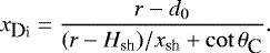
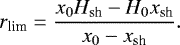
It is clear from above that as r →∞, xDi → xsh. Moreover, up to some radius, radiation from the outer disc will never reach the axis of the jet. If the distance above the disc up to which the outer disc radiation does not reach the axis is rlim, then
 (24)
(24)
2.4 Method of obtaining solutions
The jet solutions can be obtained by integrating Eqs. (13) and (14). Since, the jet originates from the accretion flow from a region close to the horizon, the jet speed should be small, but because of hot base, the jet base is subsonic. At large distances from the BH, the jet moves with very high speed and is cold and hence is supersonic. If we let the jet become transonic, that is, vc = ac at the sonic point, (r = rc). Here suffix c denotes quantities on the sonic point. Further, at rc, d v∕dr → 0∕0, which enables us to write down sonic point conditions as
 (25)
(25)
and
 (26)
(26)
At rc, d v∕dr is obtained by L′ Hôpital’s rule. Equation (26) gives functional dependence of the sound speed on rc, from which Θc, the temperature at the sonic point, can easily be obtained. Θc can be used to determine all other parameters at the sonic point, such as ac and  (using Eqs. (4) and (10)). Since E has no exact analytical form, it is obtained by numerical integration. Moreover, E is a constant of motion and
  an integration constant for the present case; one can supply either and obtain the value of rc, or, with values of rc, one may calculate all the flow quantities, and start integrating using Rung–Kutta’s fourth-order method from rc, inwards and outwards, to obtain the solutions. To determine density, one may need to explicitly supply Ṁo which are a few percent of accretion rates, as has been theoretically obtained (Chattopadhyay & Kumar 2016; Kumar & Chattopadhyay 2017).
The existence of multiple sonic points in the flow opens up the possibility for the formation of shocks in the flow. At the shock, the flow is discontinuous in density, pressure, and velocity. The relativistic Rankine-Hugoniot conditions relate the flow quantities across the shock jump (Taub 1948; Chattopadhyay & Chakrabarti 2011)
![Mathematical equation: \begin{equation*} [{\rho}u^r]= [\dot{E}]=[T^{rr}_M+T^{rr}_R]=0.\end{equation*}](/articles/aa/full_html/2018/06/aa31830-17/aa31830-17-eq54.png) (27)
(27)
Dividing Ė and Trr conservationconditions by mass conservation equation followed by a little algebra leads to
![Mathematical equation: \begin{equation*} \left[\left(h \gamma v+\frac{2 \mathrm{\Theta}}{\tau \gamma v}\right)\right]=0;~\textrm{and}~ [E]=0.\end{equation*}](/articles/aa/full_html/2018/06/aa31830-17/aa31830-17-eq55.png) (28)
(28)
We check for shock conditions (Eq. (28)), as we solve the equations of motion of the jet. However, one should note that unlike VC17, the thermal energy (− hut) doesn’t remain conserved across the shock and the corresponding conserved quantity is generalized Bernoulli parameter E.
3 Analysis and results
3.1 Nature of radiative moments
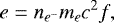
In Fig. 2a–c, we plot radiative energy density R0, flux R1, and radiative pressure R2 as functions of r. The components of the radiation field presented in all the panels are for ṁ = 10 which corresponds to a corona size of xsh = 12.31 (see Eq. (A.3)). The luminosity of such an accretion disc is ℓ = 0.8 around a BH of MB = 10 M⊙. In Fig. 2a, we plot coronal moments RnC (in compact notation) from discs around MB = 10 M⊙. The moments from the corona dominate the radiation field close to the BH. Further, because the corona is geometrically thick, the radiation flux (R1C) is negative within the funnel like region and is therefore likely to oppose the jet flowing out, along with the radiation drag terms (negative terms in right-hand side of Eq. (7)). Figure 2b shows moments (presented in compact notation RnD) from the outer disc. Because of the shadow effect from the corona, all moments of the outer disc are zero for r ≤ rlim(= 30) obtained from Eq. (24). The moments of the outer disc for ṁ peak aroundr = 55. In Fig. 2c, we plot the total radiative moments from the outer disc and the corona. Far away from the BH (r > few × 102), the jet sees the disc like a point source and all moments fall like the inverse square of the distance, and at such distances R0 ~ R1 ~ R2.
The radiation field in VKMC15 was calculated assuming flat space as pNp do not take care of the impact of gravity in radiation fields. In Fig. 3, we compare radiative moments calculated in flat space with curved space for ℓ = 2.25. The various curves represent energy density R0, R0F, R1, R1F, R2, R2F. Moments in curved space, Rn, are different from that in flat space, RnF, due to the presence of metric components. The metric components related to the accretion disc coordinates enter inside the integral while calculating radiative moments (Eq. (22)). The appearance of n as a power in Eq. (22) shows that the curvature effects are different for different moments. Further, the metric component grr appears inside the radiative term while determining ℘. This means that the curvature affects the radiative term in a very complicated way. In order to quantify the difference curvature has on the radiative terms, we compare the radiation drag term  in the curved space with its version in the flat space
 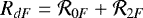 in Fig. 4, for the same luminosity as in Fig. 3. The difference is clearly visible. At r >~ 2 the drag term |Rd |>> |RdF|, but at r > 3.5 the curvature effect changes in an opposite manner, that is, Rd < RdF. At 8 ~ r ~ 9, RdF ~ 1.3Rd, which is the maximum deviation from the curved space values. However, the most interesting thing is that the drag term computed inthe flat space is about three percent more than that computed in the curved space, even at a distance of about one hundred gravitational radii. In other words, not only does the curvature affect the radiative moments at moderately large distance, but since deviation varies with distance, one cannot use a scale factor to incorporate the curvature effect on radiation in flat space.
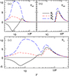 |
Fig. 2 Distribution of radiative moments-energy density R0 (long dashedblue line), flux R1 (solid black line) and pressure R2 (dashed red line) with r above an accretion disc with ṁ = 10. Radiative moments produced by various components of the disc, for example, (a) from corona RnC; (b) from outer disc RnD and (c) total radiative moments Rn. |
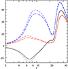 |
Fig. 3 Energy density R0 (long dashedblue line) R0F (dashed blueline), R1 (solid black line) R1F (dotted black line), R2 (long, dashed-dotted red line) R2F (dashed-dotted red line) for ℓ = 2.25. Quantities with subscript F denote moments calculated in flat space |
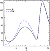 |
Fig. 4 Comparison of radiation drag term Rd computed incurved space (solid black line) and flat space (dashed blue line) for the moments shown in Fig. 3. |
3.2 Nature of sonic points
We present Θc (Fig. 5a) and ac (Fig. 5b) as functions of rc. Each plot represents sonic point properties of jets in a radiation field of an accretion disc with luminosities ℓ = 2.85, ℓ = 0.13, and ℓ = 0.0, or a thermally driven jet. Physically, different values of rc imply different choices of boundary conditions that give different transonic solutions. In the absence of radiation, Eq. (26) reduces to sonic point condition for thermal jets [ ]. This implies, for the physical values of ac, that is,
  , that the range of sonic points is 3rg < rc < ∞. In the presence of radiation, the range of sonic points reduces to 3 < rc < rl (some finite distance), as shown in Fig. 5a, b. The case with ℓ = 0.13 almost follows the curve for thermal jets until about 50rg, where it deviates and terminates at a distance of ~100rg. The sonic point properties (i.e. Θc and ac) for ℓ = 2.85 are significantly different from the thermal jet and terminate at 14rg.
It is worth mentioning that in VKMC15 there were no sonic points in the range 3–4rg. Hence solutions in the present paper in which sonic points are in the range 3rg < rc < 4rg, cannot be found in VKMC15 (Appendix B). This is because using pNp to mimic strong gravity makes the flow unphysically hot. As a result there is enhanced thermal acceleration in all the solutions of VKMC15 compared to the present one.This highlights one of the drawbacks of combining special relativistic analysis with Paczyński-Wiita potential.
The ac − rc curve in Fig. 5b forms a “knee”-like structure and rapidly decreases such that at some rc → rcf, ac → 0. At the “knee”, dac∕drc →∞ and the curve bulges slightly, although not perceptible in the figure. Truncation of rc was also seen in special relativistic (VKMC15) and pseudo-Newtonian studies (Chattopadhyay & Chakrabarti 2000a) of radiatively driven jets. The estimation of rcf can be obtained from Eqs. (25) and (26) by imposing a small ac,
 (29)
(29)
In this paper, all the solutions corresponding to the sonic points under the “knee” are called “f”-type solutions while solutions above the “knee” are referred to as “e”-type solutions, as marked in Fig. 5b.
In Fig. 6a, b we plot Ec and  as functions of rc, respectively. Various curves correspond to ℓ = 2.85, ℓ = 2.26, ℓ = 1.76, ℓ = 1.26, and ℓ = 0.28. VC17 showed that for thermal flows with conical jet geometry, Ec and
  were found to be monotonic functions of rc. In this paper, Fig. 6a, b show that Ec and
  of radiatively driven conical jets are non-monotonic functions of rc. Above a certain value of ℓ (Fig. 6a), each curve has a maximum and a minimum. For a given E = Ec and ℓ within the two extrema, there is a possibility of forming three sonic points (for curves with parameters ℓ = 2.85, 2.26, 1.76), where inner and outer sonic points are saddle-type, while middle sonic points are of spiral type. Each of the sonic points for a given E and ℓ has different entropy (
 ). Similarly, for a given choice of
  and ℓ (Fig. 6b), there is a possibility of three sonic points, differentiated by Ec.
 |
Fig. 5 Variation of Θc (panel a) and ac (panel b) with rc for a jet acted on by ℓ = 2.85 (solid black line), 0.13 (long dashed blue line) and thermal jet (dashed red line). The jet is composed of electrons and protons (ξ = 1). |
 |
Fig. 6 Panel a: Ec and panel b: |

3.3 Jet solutions
We follow procedures described in Sect. 2.4 to obtain jet solutions and in Fig. 7a–d we present a typical jet solution characterized by generalized Bernoulli parameter E = 1.04 and the composition of the flow is ξ = 1 or e − −p+ flow. In Fig. 7a, three-velocity v and sound speed a are plotted. The jet is transonic, starting with low v and high a and ending with the opposite, respectively. Interestingly, R1 > 0 for r > 20 above a disc and the jet starts to accelerate significantly above that distance. The radiation field is for ℓ = 0.8. In Fig. 7b, we compare v of a thermally driven jet with v of a radiatively driven jet, where vT of the radiatively driven jet is about twice greater than that of the thermal jet. The temperature of the radiatively driven jet decreases by five orders of magnitude over a distance scale of five orders of rg (Fig. 7c) and consequently Γ increases from a relativistic value to a non-relativistic one (Fig. 7e). The constant of motion E is plotted in Fig. 7d and since the flow is isentropic,  is also constant (Fig. 7f).
Radiation from a luminous disc resists the jet within some distance above the funnel of the corona, but drives the flow beyond it. As a result, multiple sonic points are formed in jets at high ℓ for all values of E within the maxima and minima in each of the Ec –rc curves (Fig. 6a). Therefore, the loci of the maxima and the minima marks the range of E and ℓ for which the flow harbours multiple sonic points demarcated by XYZ in Fig. 8a. The region UZV (dotted, blue) represents flow parameters for which a jet has stable shock solution. In Fig. 8b–g we plot the Mach number M = v∕a as a function of r, where each panel corresponds to the coordinate points marked as “b”–“g” in E–ℓ parameter space in Fig. 8a. Here all possible jet solutions are presented, but for the sake of completeness, we have also plotted the inflow solutions. The crossing points denote the locations of the X-type sonic points. If the jet is illuminated by low-luminosity radiation, then it flows out through only one sonic point (Fig. 8b, c). If the jet is driven by high-luminosity radiation, then for lower energies, it will pass through a single outer-type sonic point (Fig. 8d, e). However, for higher ℓ and E, the jet may possess multiple sonic points (Fig. 8g, f). In Fig. 8g the jet undergoes shock transition, but in Fig. 8f it flows out only through the outer sonic point. The inner and outer sonic points are X type and the middle one is spiral type (Fig. 8f, g). Figure 8d is of special importance, since these are “f”-type jets which start with very low velocities but achieve relativistic terminal speeds.
It is interesting to note that the radiation effect is more perceptible for low-energy jets than for higher-energy ones. To elaborate, we once again invoke the Ec —rc curve in Fig. 9a for jets acted on by three disc luminosities ℓ = 2.85, ℓ = 0.8, 0.035, and mark three energy values as “b” at E = 2.71, “c” at E = 1.04, and “d” at E = 1.7. We compare the jet solutions at each of these values of E in panels b, c and d in Fig. 9. At high energies (i.e. Fig. 9b), radiation has no driving power due to the presence of enthalpy in the denominator of the radiation term (Eq. (15)). The thermal gradient term in such cases is so strong that it accelerates the jet close to its local veq (Eq. (17)). Therefore, shining radiation will only increase the radiation drag term and reduce the speed, as is seen in this panel. Near the base, jets for all three ℓ achieve almost the same v. As the temperature falls and  starts to become effective, jets plying through field with higher radiation are slower. Radiation is quite effective for low-energy jets (Fig. 9c). Within the funnel R1 is negative, therefore, the higher the luminosity of the disc, the greater the deceleration of jets inside the funnel. But above the funnel where R1 > 0, radiation from luminous disc will drive jets to higher terminal speeds. For middle energies, for example, E = 1.71 (Fig. 9d), the effect of radiation is even more intriguing. In the presence of low-luminosity radiation field, jets with moderate energies are thermally driven to achieve relativistic terminal speeds which are similar to the value achieved by purely thermally driven jet. Increasing ℓ increases radiation drag and the jet speeds are suppressed, reducing the terminal speed. But for even higher ℓ, the negative R1 is strong enough to cause a shock transition in the jet. In the post-shock flow, because v is significantly less than veq, there is significant acceleration and the jet achieves approximately the same terminal speed as the thermally driven jet. Therefore, for fluid jet, the role of radiation momentum deposition has multiple consequences with distinctly different outcomes, which underlines the importance of this study.
The definition of terminal speed or vT is the asymptotic jet speed, that is, at r → large, v → vT where d v∕dr → 0. In Fig. 10a, we plot vT of jets with ℓ for three energies E = 2.71, E = 1.71 and E = 1.04. For low-energy jets, terminal speed increases with ℓ. While for very high-energy jets, radiation drag decelerates the jet and vT decreases with ℓ. For moderate values of E, radiation decelerates the jet whenℓ is low, but for higher ℓ, R1 within the funnel opposes the outflowing jet to such an extent that it triggers a shock transition. In the post-shock jet, v is significantly less than veq and R1 > 0, therefore radiation accelerates the jet efficiently to achieve high vT. In Fig. 10b, we plot vT as a function of E, where each curve represents ℓ = 2.85 and ℓ = 0.8. Similar to the previous panel, we find vT increases with ℓ for lower E and decreases for higher E. It is interesting that for high E, vT is greater for lower ℓ. We also define an amplification parameter Am = vT∕vb as a measure of acceleration of the jet, where vb is the base speed with which the jet is launched. In Fig. 10c, we plot Am as a function of E for ℓ = 0.8. The dotted part of the curve represents “f”-type solutions and the solid curve represents “e”-type solutions. It is clear from the plot of the amplification parameter that radiation driving is more effective for “f”-type solutions, compared to the “e”-type jets.
Since the jet also contains radiation driven shock, so we plot the shock location Rsh (Fig. 11a), compression ratio R (Fig. 11b), and shock strength S (Fig. 11c) as a function of E with each curve plotted for constant values of ℓ. The compression ratio is defined as R = ρ+∕ρ− (the ratio of post and pre-shock mass densities); and the shock strength S =M−∕M+ (the ratio of pre- and post-shock Mach numbers). The composition of the jet is ξ = 1.0 and each curve is for ℓ = 2.26 and ℓ = 2.85. In general, Rsh increases with E, because higher E implies higher thermal energy at the base which pushes the shock front outwards. In jets, as the shock moves outwards, the jump condition becomes steeper and hence the shock becomes stronger. VC17, which also showed the existence of shocks, was consistent with the above fact. However, the crucial difference between VC17 and the present venture is the agent that drives the shock. In VC17, the shock is driven by the geometry of the flow and is coupled with the thermal term (the coefficient of a2 in Eq. (17) of VC17) and therefore, the shock becomes stronger with E. In the present paper, the shock is driven by the radiation that opposes the jet flow within the funnel of the disc. In addition, the radiation term  is more effective for flows with lower thermal content, that is, with lower E. Therefore, increasing E would negate the effectiveness of radiation, and should weaken the shock. So R and S, which measure shock strength, initially increase but eventually decrease with increasing E, maximizing at some value of E in stark contrast with VC17. It is also quite clear that for higher ℓ, the shock generally becomes stronger (long-dashed and solid curves).
A closer look into Eq. (15) reveals that  is twice as large for e−− e+ jets as for e − −p+ jets for the same values of Θ and v. Lepton-dominated flows have been shown to be colder than e−−p+ flows (Chattopadhyay & Ryu 2009; Chattopadhyay & Chakrabarti 2011), which means that the term f + 2Θ is lower for low ξ flow. In other words,
 will be more effective for lepton-dominated jets. However, one cannot compare jets with same E across a range of compositions. If one considers Eq. (11), then one can easily understand that a slight change in Xf will affect the value of E by a large amount. Since for low ξ flow, Θs are quite different from those of e−−p+ flow, jets with different ξ, starting with similar temperature and velocity, will have widely differing E. In Fig. 12a we compare jets launched with the same velocity at the base and driven by radiation of the same luminosity (ℓ = 2.85), each curve corresponds to ξ = 1.0, ξ = 0.6, ξ = 0.15, and ξ = 0.05. Jet speeds are higher for flow with lower ξ. In Fig. 12b, we plot vT of the jet with the flow composition ξ; each curve corresponds to super-Eddington luminosity (ℓ = 2.85) and sub-Eddington luminosity.
 |
Fig. 7 Panel a: three-velocity v (solid black line) and sound speed a (long dashedblue line) as functions of r. Panel b: comparison of velocity distribution of thermally driven or ℓ = 0 jet (dashed red line) and the radiatively driven jet (solid black line); panel c: Θ;panel d: E; panel e: Γ and panel f: |

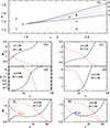 |
Fig. 8 Panel a: E − ℓ parameter space: bounded region XZY signifies parameters for multiple sonic points in jet and region UZV within bluedotted lines represents parameters for which flow goes through shock transition. Filled circles named “b–g” are the flow parameters E and ℓ, for which the jet solutions are plotted in panels b–g. Mach number M = v∕a is plotted as a function of r for b) E = 1.46, ℓ = 1.25; c) E = 1.208, ℓ = 1.25; d) E = 1.208, ℓ = 2.26; e) E = 1.39, ℓ = 2.26; f) E = 1.47, ℓ = 2.26; and g) E = 1.5, ℓ = 2.26. Each panel shows physical jet solutions (solid black line) and corresponding inflow solutions (dashed red line). Sonic points are shown by the crossing of inflow and jet solutions. All solutions are for e − − p + flow. |
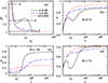 |
Fig. 9 Panel a: Ec–rc plot with energy levels marked as “b” at E = 2.71, “c” at E = 1.04 and “d” at E = 1.7. Panel b: comparison of three-velocity v as a functionof r of jets starting with E = 2.71. Panel c: comparison of v for “f”-type jets with E = 1.04; and, panel d:comparison of v for jets with E = 1.7. Each curve corresponds to ℓ = 2.85 (solid black line), 0.8 (long dashedblue line) and 0.035 (dashed red line). The composition of the jet is ξ = 1 or e − −p+. |
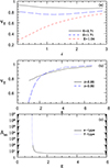 |
Fig. 10 Panel a: variation of vT with ℓ. Various curves represent E = 2.71 (solid black line) E = 1.71 (long dashedblue line) and E = 1.04 (dashed red line). Panel b: vT as a functionof E for different ℓ = 2.85 (solid black line) and 0.8 (dashed red line). Panel c: amplification factor Am with E of jets flowing out through a radiation field of ℓ = 0.8. All panels have ξ = 1. The “e”-type(solid line) and “f”-type (dotted line) jets are also marked. |
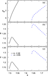 |
Fig. 11 Panel a: jet shock location Rsh; panel b: compression ratio R and panel c: shock strength S as a functionof E for jets with composition ξ = 1.0. Each curve is for ℓ = 2.26 (solid line) and ℓ = 2.85 (long-dashed line). |
 |
Fig. 12 Panel a: v as a functionof r for jets actedon by disc radiation marked by ξ = 1.0 (solid black line); ξ = 0.6 (long-dashed blue line), ξ = 0.15 (dashed red line) and ξ = 0.05 (dotted magenta line). The disc radiation is for ℓ = 2.85. Panel b: variation of vT with ξ for “f”-type jets, driven by radiation quantified by ℓ = 2.85 (solid line) and ℓ = 0.8 (dashed line). |
4 Discussion and conclusions
Here we study radiatively and thermally driven jets with spherical cross section having a small opening angle around BH. Since the flow is hot enough to be fully ionized, the momentum transferred from radiation to the jet is only through scattering. The thermodynamics of the jet is described by a relativistic EoS, while it flows through the radiation field of the accretion disc in Schwarzschild metric. The disc assumed has a thick compact corona, which emits through bremsstrahlung and synchrotron processes like the outer disc, but additionally, through the inverse-Compton process, all of which is implemented via a fitting function.
Generally, most of the studies on radiatively driven jets are conducted in SR regime and stronger gravity is mimicked by adding any gravitational potential adhoc in the momentum balance equation (FTRT85; VKMC15). Even if we overlook the obvious mistake of combining SR and any gravitational potential from the view point of the famous Principle of Equivalence, still it produces many unphysical phenomena in the solutions. For example, the adhoc gravity in the SR-regime produces unrealistically hot jets, such that sonic points do not form within four Schwarzschild radii. Even in cases where transonic solutions are obtained, the thermal gradient term completely dominates the radiation term. This accelerates the jets to reach their local equilibrium velocity. Hence, further out, when the jet is cooler, radiation drag becomes more important than radiation driving. In proper GR regime, the radiation drag at moderate distances is much lower.
Since we are considering curved space-time in the present paper, consequently the radiative moments have been computed by implementing the SR and curved space-time transformations on the specific disc intensities and directional derivatives; as expected, the curvature in space reduces the magnitude of the radiative moments. However, the effect of radiation is more complicated than meets the eye. The radiation drag term, when computed in GR regime, overwhelms near the horizon because of the presence of the 1∕grr term, but is lesser than that computed in flat space-time, further out. Crucially, this non-linear difference of the drag term between GR and flat space cannot be mimicked by some simple scaling relation.
In the advective disc model, there are two sources of radiation – the inner compact corona and the outer disc. The accretion rate not only controls the overall radiative output from the disc, but also determines the size of the corona. Since we are considering Thomson scattering regime, the details of the spectrum do not matter and frequency integrated moments of the radiation field suffice. The radiative moments generally have two peaks corresponding to the radiation from the corona and the outer disc (Fig. 2). A comparison of the moments for an accretion disc with an inner corona and outer KD (Chattopadhyay et al. 2004; Chattopadhyay 2005) with the present disc model shows that the radiative moments computed from the outer disc of the present model are much stronger.
In this paper, we compute the generalized, relativistic Bernoulli parameter (E) for radiatively driven flow in curved space time. This is a constant of motion even in the presence of radiation driving. The expression of relativistic Bernoulli parameter (≡−hut) for adiabatic and isentropic flow is not conserved along the streamline of a radiatively driven flow or across the shock, but E is a constant of motion. This gives us a great tool to find various classes of solutions. One must not confuse E with the generalized relativistic Bernoulli parameter obtained for accretion discs (Chattopadhyay & Kumar 2016; Kumar & Chattopadhyay 2017). Since the streamline and various dissipative processes in an accretion disc are different from the jet (compare Xf of Eq. (11) of this paper and Eq. (18) of Chattopadhyay & Kumar 2016), the values of generalized Bernoulli parameters will not be the same for both jet and accretion disc, even if the jet is launched with the local accretion disc variables on the foot points of the jet.
In this paper, unlike (VKMC15), we consider hotter and therefore geometrically thicker corona. This has a very interesting radiative flux (R1) distribution. Within the funnel ofthe corona, R1 < 0 and therefore opposes the out-flowing jet. Above the height of the corona, R1 > 0 and it pushes the jet outward. That the radiation accelerates can be understood from the fact that the range of sonic points becomes limited, with the increase of disc luminosity. If E is high, then the jet is hot at the base and the effect of radiation is negligible. Thermal driving completely dominates within the funnel and accelerates the jet such that v ~ veq. Above the funnel the jet is sufficiently cooled, such that the radiative term starts to become effective, but since the jet has reached up to the local equilibrium speed, radiation deceleration would actually slow the jet down (Figs. 9b and 10a). For medium and small values of E, thermal and radiation driving may accelerate jets to relativistic speeds and the speed increases with the disc luminosity. In fact, for lepton-dominated flow (ξ = 0.01) jets do reach γT >~ 10. But more than acting simply as an agent of acceleration/deceleration, radiation does trigger a shock transition in jets very close to the BH. The shock range is small and the shock strength is moderate and peaks at certain values of jet energy for a given disc luminosity. It may be noted that shocks generated in this paper are triggered by the inwardly directed radiation flux within the funnel of the corona, which is different from the shocks generated by “pinching off” the flow geometry in VC17.
Radiatively driven fluid jet in relativity has a very rich class of solutions. The “e”-type solutions may have one inner-type sonic point, multiple sonic points, and shocks. While the “f”-type jet is a low-energy solution, such solutions pass through the outer sonic point. The radiative driving is the most effective for “f”-type jet solutions (Fig. 12a). This class of solutions can be compared with radiatively driven e− − e+ jets in the particle approximation (Chattopadhyay et al. 2004; Chattopadhyay 2005). Interestingly, discs with sub-Eddington luminosity can power lepton-dominated jets (ξ = 0.01) to terminal Lorentz factors γT ~ 3, but super-Eddington discs can power those “f”-type jets to γT ~ 10 (Fig. 12b). Above, we argued that the radiation driving of particle jets is more efficient than that of fluid jets due to the presence of the enthalpy term in the denominator of the radiation term (Eq. (15)). However, the advantage of considering radiation driving of fluid jets is that wherever the jet has been hot, radiation driving is not effective, but the thermal gradient term is. In the region where the temperature falls down, thermal gradient becomes less effective, but radiation takes over, provided the region is relatively close to the disc (~100rg). Therefore, the lepton-dominated jets achieve terminal speeds similar to the e− − e+ particle jets, and, in addition, the radiation driving can produce fluid phenomena like shocks in the jet. An unstable shock can also produce effects like QPOs in the jet, a scenario worth investigating. Moreover, such internal shocks close to the jet base have been invoked to explain the high-energy power-law tails in some of the microquasars (Laurent et al. 2011). FTRT85 also showed the existence of shocks in radiatively driven jets, when the disc is quite thick and jet geometry deviates from the conical geometry. Although the authors were not considering the effect of acceleration of radiation on jets, the vT quoted by them were all mildly relativistic (vT ~ 0.1). Whereas, in our paper, we find vT is a few times higher in general, the reason being FTRT85 considered mostly isothermal jets and therefore missed the thermal driving factor for the jet. Our present work is also different from Meliani et al. (2004) since the accelerating agent in their work was hidden within the equation of state. They also did not find any fluid discontinuities such as shock in the jets.
We conclude by stating that radiation is an important agent in triggering various physical processes in a jet. The radiation can drive e− –p+ jets to reasonable terminal speeds (vT >~ 0.5) if the disc is sub-Eddington. However, for very hot jets under intense radiation field, γT ~ 3 is achievable. For lepton-dominated flow and intense radiation field γT ~ 10 is also possible. The response of jet terminal speed with disc luminosity is not straight forward; vT may slightly decrease with increasing luminosity for high-energy jet, it may decrease and then increase with increasing luminosity for moderate-energy jets, but will increase with ℓ for low-energy jets. It may be worth noting that radiation may accelerate jets to relativistic terminal speeds, contrary to what is popularly accepted (Guthmann et al. 2002).
Acknowledgements
The authors acknowledge the anonymous referee for raising pertinent issues which helped to improve the quality of the paper. The authors also acknowledge ARIES for supporting this work.
Appendix A Accretion disc and associated radiation parameters
A.1 Estimating approximate accretion disc variables
Uμ are the components of accretion four-velocity, and the corresponding three-velocity components are v ≡ (ϑx, 0, ϑϕ), where x, θ, and ϕ are usual spatial coordinates. We define  as the radialthree-velocity measured by a local rotating observer. Following this, one can present the velocity distribution of the outer disc and the corona in a compact form (see Appendix A of VKMC15)
![Mathematical equation: \begin{equation*} \vartheta_{\textrm{i}}=\left[1-\frac{(x-2)x^2}{\{x^3-[(x-2)\lambda^2]\}U_t^2|_{x_{0\textrm{i}}}} \right]^{1/2},\end{equation*}](/articles/aa/full_html/2018/06/aa31830-17/aa31830-17-eq72.png) (A.1)
(A.1)
where the suffix i denotes variables of the corona (i.e. i = C) or the outer disc (i.e. i = D) and  is the covariant time component of the Uμ at the outer edge. For the corona, x0i = xsh and for the outer disc x0i = x0. At x0,
 ![Mathematical equation: $ [\vartheta_{\textrm{\small D}}]_{x_0} \approx 0$](/articles/aa/full_html/2018/06/aa31830-17/aa31830-17-eq74.png) but increases as it falls towards the BH until it reaches xsh, where the flow speed reduces by one-third. In shocked accretion disc, this reduction is automatic, but even in shock-free discs, centrifugal barrier and radiation pressure can both impede the inflow, making it hot and thereby forming the corona. Assuming a slow variation of the adiabatic index the temperature distribution can also be assumed as (VKMC15)
but increases as it falls towards the BH until it reaches xsh, where the flow speed reduces by one-third. In shocked accretion disc, this reduction is automatic, but even in shock-free discs, centrifugal barrier and radiation pressure can both impede the inflow, making it hot and thereby forming the corona. Assuming a slow variation of the adiabatic index the temperature distribution can also be assumed as (VKMC15)
 (A.2)
(A.2)
Moreover, VKMC15 proposed an approximate relation between xsh and the accretion rate, given by
 (A.3)
(A.3)
Here xsh is in geometric units and ṁ is the accretion rate in units of Eddington rate (Eddington rate ≡ ṀEdd = 1.4 × 1017 MB∕M⊙ g s−1). In order to completely specify ϑi and Θi at all x, one also needs to know the local height Hi. Numerical simulations show that the outer disc has a flatter structure than that predicted by assumptions of vertical equilibrium and the inner torus like corona is basically a thick disc (with advection terms) and the height to radius ratio can vary between 1.5 and 10 (Das et al. 2014; Lee et al. 2016). Therefore, we define H0 = 0.4Hsh + tanθDx0. If we supply ![Mathematical equation: $[\vartheta_{\textrm{\small D}}]_{x_0},~\rho_0,~H_0$](/articles/aa/full_html/2018/06/aa31830-17/aa31830-17-eq77.png) and ṁ at x0, then the distribution of velocity, temperature, density at all xi, as well as the location of xsh, can be estimated. Typical accretion disc parameters are given in Table A.1.
and ṁ at x0, then the distribution of velocity, temperature, density at all xi, as well as the location of xsh, can be estimated. Typical accretion disc parameters are given in Table A.1.
Disc parameters.
A.2 Radiative intensity and luminosity from the accretion flow
The outer disc emits mainly via synchrotron and bremsstrahlung processes and the corona additionally via inverse-Compton process. The functional form of the frequency integrated local intensity of the outer disc is given by (Kumar & Chattopadhyay 2014; VKMC15),
![Mathematical equation: \begin{eqnarray*} &{\tilde I}_{\textrm{\small D}}&={\tilde I}_{\textrm{syn}}+{\tilde I}_{\textrm{brem}} \nonumber \\* & &=\left[\frac{16}{3}\frac{e^2}{c}\left( \frac{eB_{\textrm{\small D}}}{m_e c} \right)^2 \mathrm{\Theta}^2_{\textrm{\small D}} n_{\textrm{\small D}} x+ 1.4\times 10^{-27}n_{\textrm{\small D}}^2g_bc \sqrt{\frac{\mathrm{\Theta}_{\textrm{\small D}} m_e}{k}}\right] \nonumber \\* &&\quad\times\, \frac{\left(d_0 \sin \theta_{\textrm{\small D}}+x\cos \theta_{\textrm{\small D}} \right)}{3} \ \ \textrm{erg} \ \textrm{cm}^{-2}\, \textrm{s}^{-1}.\end{eqnarray*}](/articles/aa/full_html/2018/06/aa31830-17/aa31830-17-eq78.png) (A.4)
(A.4)
Here, ΘD, nD, x, θD, BD and  are the local dimensionless temperature, electron number density, radial distance of the disc, the semi-vertical angle of theouter disc surface, the magnetic field, and the relativistic Gaunt factor, respectively. Intensity is measured in the disc local rest frame. The factor outside square brackets converts emissivity (erg cm−3 s−1) into intensity (erg cm−2 s−1). The luminosity of the outer disc is obtained by integrating I0 over the disc surface, that is,
 (A.5)
(A.5)
which can be presented in units of LEdd(≡ 1.38 × 1038 MB∕M⊙ ergs s−1) as ℓD = LD∕LEdd. Since the accretion disc solution has been approximated, we do not calculate the radiation from corona directly, but instead estimate it from the enhancement factor computed from self-consistent two-temperature solutions (Mandal & Chakrabarti 2008). The ratio of corona and outer disc luminosities is computed following Mandal & Chakrabarti (2008) and was presented in VKMC15,
 (A.6)
(A.6)
We assume that these functions are generic. Therefore, the luminosity from the corona can be estimated as LC = χLD, and the dimensionless total luminosity is given by
 (A.7)
(A.7)
The specific intensity measured in the local rest frame of the corona is given by ĨC = LC∕πAC. The dimensionless form of σTĨC∕me is given by
 (A.8)
(A.8)
Here AC is the surface area of the corona. To obtain the specific radiation intensities (Eqs. (A.4) and (A.8)) from the accretion disc, we need the number density and temperature distribution of the disc. Here, ĨC is obtained from ĨD, in which nD is obtained by supplying ṁ from Eq. (A.1) and ΘD from Eq. (A.2). In this paper, we have only concentrated on accretion discs around MB = 10 M⊙.
Appendix B Paczyński-Wiita potential (PW) and relativistic flows
More often, radiatively driven relativistic jets are studied in the SR plus PW regime and not in GR regime. Although the Equivalence Principle strictly precludes this possibility, in astrophysics this trend has been followed by a number of researchers because it isassumed that GR affects only in the region outside the BH and not at moderate to large distances. Here we show that the differences in equations in the two approaches affect the solutions close to the BH, as well as at moderate distances (few × 10rg). Moreover, the temperature produced in SR+PW regime is unphysically high. Furthermore, radiation effects in curved space time cannot be properly taken into account by any scaling relations, if the moments are computed in the flat space. The effect of curvature inthe radiation term is addressed in Sect. 3.1. Therefore, we list the first two points below.
B.1 Equations of motion
The equations of motion in the two approaches can be written down as
![Mathematical equation: \begin{align*} &\gamma^4v\left(1-\frac{a^2}{v^2}\right)\left[\frac{\mathrm{d}v}{\mathrm{d}r}\right]_{\mathrm{GR}}=\frac{2a^2 \gamma^2}{r}-{\frac{\left(1-a^2\right)\gamma^2}{r(r-2)}} +\,\frac{(2-\xi)\gamma^3}{(f+2\mathrm{\Theta}){ \sqrt{g^{rr}}}} \nonumber \\ &\quad\quad\quad\quad\quad\quad\quad\quad\quad\left[(1+v^2){{\cal R}_1}-v {\left(g^{rr} {\cal R}_0+\frac{{\cal R}_2}{g^{rr}}\right)}\right],\end{align*}](/articles/aa/full_html/2018/06/aa31830-17/aa31830-17-eq84.png) (B.1)
(B.1)
and
![Mathematical equation: \begin{align*} &\gamma^4v\left(1-\frac{a^2}{v^2}\right)\left[\frac{\mathrm{d}v}{\mathrm{d}r}\right]_{\mathrm{PW}}=\frac{2a^2 \gamma^2}{r}-{\frac{1}{{(r-2)^2}}} +\frac{(2-\xi)\gamma^3}{(f+2\mathrm{\Theta})} \nonumber \\ &\quad\quad\quad\quad\quad\quad\quad\quad\quad\left[(1+v^2){{\cal R}_{1F}}-v { \left({\cal R}_{0F}+{\cal R}_{2F}\right)}\right].\end{align*}](/articles/aa/full_html/2018/06/aa31830-17/aa31830-17-eq85.png) (B.2)
(B.2)
The subscript PW signifies equations of motion in SR+PW regime, while GR represent the equations in Schwarzschild metric. Values with subscript F are calculated in flat space. The right-hand side of both Eqs. (B.1) and (B.2) algebraically differ in the second term of the numerator, and the presence of curvature grr in the radiation terms. Since the form of the first terms are the same, let us take the ratio of the second terms on the right-hand side of the abovetwo equations,
The calculations with SR+PW potential will be comparable to GR if δ ~ 1. For relativistic winds or jets at large distances, grr ≈ 1, a is very low, but v → 1, meaning that

Similarly close to the BH, that is, r → 2, grr → 0, v ≈ 0, but a is large, therefore

This analysis points to the possibility of a large deviation from GR solutions even at larger distances. This difference in the second term of the EoMs arises because in SR+PW regime the gravity enters as an additive term (Eq. (B.2)), whilein GR it is a space time phenomena (Eq. (B.1)) so it affects any source of energy. Therefore, the curvature term (gμν s) should couple with the thermal and the kinetic terms as is seen above, that is, the curvature term is coupled with the thermal term in the form of sound speed a and also the Lorentz factor γ. Consequently, if there is a discontinuity such as shock in the flow, then the gravity term in SR+PW will not change across the shock, but in GR it will change, since both a and v jump across a shock. Further,Abramowicz et al. (1996) also showed that even in accretion problems, SR and PW potential are not compatible.
B.2 Overestimated thermal content in PW analysis
Causality imposes an upper limit on sound speed which is  . In GR this translates to a lower bound in the location of sonic points (rc > 3). This is clear in Fig. 5. Since pseudo potentials make the flow unphysically hot, the lower limit of sonic point in pNp+SR regime extends to a larger distance (rc > 4). For thermally driven flow this can be very easily shown. From Eqs. (B.1) and (B.2) and ignoring radiation, we obtain ac as a function of rc.
![Mathematical equation: \begin{equation*} [a_c]^2 _{\textrm{GR}}=\frac{1}{2r_c-3}, \end{equation*}](/articles/aa/full_html/2018/06/aa31830-17/aa31830-17-eq90.png) (B.3)
(B.3)
![Mathematical equation: \begin{equation*} [a_c]^2 _{\textrm{PW}}=\frac{r_c}{2(r_c-2)^2+r_c}. \end{equation*}](/articles/aa/full_html/2018/06/aa31830-17/aa31830-17-eq91.png) (B.4)
(B.4)
These are algebraic relations and ![Mathematical equation: $[a_c]_{\textrm{PW}}$](/articles/aa/full_html/2018/06/aa31830-17/aa31830-17-eq92.png) is higher than
is higher than ![Mathematical equation: $[a_c]_{\textrm{GR}}$](/articles/aa/full_html/2018/06/aa31830-17/aa31830-17-eq93.png) (Fig. B.1). In other words, the jet in SR+PW description is much hotter than the GR one. This also means the SR+PW jet is subjected to a much stronger thermal gradient push than it is in reality. Moreover, all jet solutions with 3 < rc ≤ 4 are absent in SR+PW solutions.
(Fig. B.1). In other words, the jet in SR+PW description is much hotter than the GR one. This also means the SR+PW jet is subjected to a much stronger thermal gradient push than it is in reality. Moreover, all jet solutions with 3 < rc ≤ 4 are absent in SR+PW solutions.
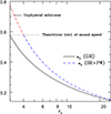 |
Fig. B.1 ac as a functionof rc for ℓ = 0. Solid curve is for GR solutions while dotted shows solutions with PW potential. |
References
- Abramowicz, M. A., Beloborodov, A. M., Chen, X., & Igumenshchev, I. V. 1996, A&A, 313, 334 [NASA ADS] [Google Scholar]
- Agudo, I., Gomez, J. L., Marti, J. M., et al. 2001, ApJ, 549, L183 [NASA ADS] [CrossRef] [Google Scholar]
- Baade, W., & Minkowski, R. 1954, ApJ, 119, 215 [NASA ADS] [CrossRef] [Google Scholar]
- Beloborodov, A. M. 2002, ApJ, 566, L85 [NASA ADS] [CrossRef] [Google Scholar]
- Bini, D., Geralico, A., Jantzen, R. T., & Semerak O. 2015, MNRAS, 446, 2317 [NASA ADS] [CrossRef] [Google Scholar]
- Chakrabarti, S. K. 1989, ApJ, 347, 365 [NASA ADS] [CrossRef] [Google Scholar]
- Chandrasekhar, S. 1938, An Introduction to the Study of Stellar Structure (Dover: New York) [Google Scholar]
- Chattopadhyay, I. 2005, MNRAS, 356, 145 [NASA ADS] [CrossRef] [Google Scholar]
- Chattopadhyay, I. 2008, Observational Evidence for Black Holes in the Universe, eds. S. K. Chakrabarti, & A. S. Majumdar, AIP Conf. Ser., 1053, 353 [NASA ADS] [CrossRef] [Google Scholar]
- Chattopadhyay, I., & Chakrabarti, S. K. 2000a, Int. J. Mod. Phys. D, 9, 57 [NASA ADS] [Google Scholar]
- Chattopadhyay, I., & Chakrabarti, S. K. 2000b, Int. J. Mod. Phys. D, 9, 717 [NASA ADS] [Google Scholar]
- Chattopadhyay, I., & Chakrabarti, S. K. 2002a, MNRAS, 333, 454 [NASA ADS] [CrossRef] [Google Scholar]
- Chattopadhyay, I., & Chakrabarti, S. K. 2002b, Bull. Astr. Soc. India, 30, 313 [NASA ADS] [Google Scholar]
- Chattopadhyay, I., & Chakrabarti, S. K. 2011, Int. J. Mod. Phys. D, 20, 1597 [Google Scholar]
- Chattopadhyay, I., & Das, S. 2007, New Astron., 12, 454 [NASA ADS] [CrossRef] [Google Scholar]
- Chattopadhyay, I., & Kumar, R. 2016, MNRAS, 459, 3792 [NASA ADS] [CrossRef] [Google Scholar]
- Chattopadhyay, I., & Ryu, D. 2009, ApJ, 694, 492 [NASA ADS] [CrossRef] [Google Scholar]
- Chattopadhyay, I., Das, S., & Chakrabarti, S. K. 2004, MNRAS, 348, 846 [NASA ADS] [CrossRef] [Google Scholar]
- Chattopadhyay, I., Sharma, M., Nath, B., & Ryu, D. 2012, MNRAS, 417, 2899 [Google Scholar]
- Curtis, H. D. 1918, Lick Obs. Pub., 13, 31 [Google Scholar]
- Das, S., Chattopadhyay, I., Nandi, A., & Molteni, D. 2014, MNRAS 442, 251 [Google Scholar]
- Doeleman, S. S., Fish, V. L., Schenck, D. E., et al. 2012, Science, 338, 355 [NASA ADS] [CrossRef] [PubMed] [Google Scholar]
- Dove, B. D., Wilms, J., Maisack, M., & Begelman, C. M. 1997, ApJ, 487, 759 [NASA ADS] [CrossRef] [Google Scholar]
- Duncan, G. C., & Hughes, P. A. 1994, ApJ, 436, L119 [NASA ADS] [CrossRef] [Google Scholar]
- Faris, B. D., Li, T. K., Liu, Y. T., & Shapiro, S. L. 2008, Phys. Rev. D, 78, 4023 [Google Scholar]
- Fender, R. P., Gallo, E., & Russell, D. 2010, MNRAS, 406, 1425 [NASA ADS] [Google Scholar]
- Ferrari, A., Trussoni, E., Rosner, R., & Tsinganos, K. 1985, ApJ, 294, 397 (FTRT85) [NASA ADS] [CrossRef] [Google Scholar]
- Fukue, J. 1987, PASJ, 39, 309 [NASA ADS] [Google Scholar]
- Fukue, J. 1996, PASJ, 48, 631 [NASA ADS] [CrossRef] [Google Scholar]
- Fukue, J., Tojyo, M., & Hirai, Y. 2001, PASJ, 53, 555 [NASA ADS] [CrossRef] [Google Scholar]
- Gallo, E., Fender, R. P., & Pooley, G. 2003, MNRAS, 344, 60 [NASA ADS] [CrossRef] [Google Scholar]
- Gierlinski, M., Zdziarski, A. A., Done, C., et al. 1997, MNRAS, 288, 958 [NASA ADS] [CrossRef] [Google Scholar]
- Guthmann, A. W., Georganopoulos, M., Marcowith, A., & Manolakou, K. 2002, in Relativistic Flows in Astrophysics (Berlin: Springer-Verlag), Lect. Notes Phys., 589 [Google Scholar]
- Hirai, Y., & Fukue, J. 2001, PASJ, 53, 285 [NASA ADS] [CrossRef] [Google Scholar]
- Hsieh, H. S., & Spiegel, E. A. 1976, ApJ, 207, 244 [NASA ADS] [CrossRef] [Google Scholar]
- Icke, V. 1980, AJ, 85, 329 [NASA ADS] [CrossRef] [Google Scholar]
- Icke, V. 1989, A&A, 216, 294 [NASA ADS] [Google Scholar]
- Junor, W., Biretta, J. A., & Livio, M. 1999, Nature, 401, 891 [NASA ADS] [CrossRef] [Google Scholar]
- Kato, S., Fukue, J., & Mineshige, S. 1998, Black-hole Accretion Disks (Kyoto: Kyoto University Press) [Google Scholar]
- Komissarov, S. S., Barkov, M. V., Vlahakis, N., & Königl, A. 2007, MNRAS, 380, 51 [NASA ADS] [CrossRef] [Google Scholar]
- Kumar, R., & Chattopadhyay, I. 2013, MNRAS, 430, 386 [NASA ADS] [CrossRef] [Google Scholar]
- Kumar, R., & Chattopadhyay, I. 2014, MNRAS, 443, 3444 [NASA ADS] [CrossRef] [Google Scholar]
- Kumar, R., & Chattopadhyay, I. 2017, MNRAS, 469, 4221 [NASA ADS] [CrossRef] [Google Scholar]
- Kumar, R., Singh, C. B., Chattopadhyay, I., & Chakrabarti, S. K. 2013, MNRAS, 436, 2864 [NASA ADS] [CrossRef] [Google Scholar]
- Kumar, R., Chattopadhyay, I., & Mandal, S. 2014, MNRAS, 437, 2992 [NASA ADS] [CrossRef] [Google Scholar]
- Laurent, P., Rodriguez, J., Wilms, J., et al., 2011, Science, 332, 438 [NASA ADS] [CrossRef] [PubMed] [Google Scholar]
- Lee, S.-J., Chattopadhyay, I., Kumar, R., Hyung, S., & Ryu, D. 2016, ApJ, 831, 33 [NASA ADS] [CrossRef] [Google Scholar]
- Leer, E., & Holzer, T. E. 1990, ApJ, 385, 680 [NASA ADS] [CrossRef] [Google Scholar]
- Mandal, S., & Chakrabarti, S. K. 2008, ApJ, 689, L17 [NASA ADS] [CrossRef] [Google Scholar]
- Marti, J. M., & Muller, E. 1997, ApJ, 479, 151 [NASA ADS] [CrossRef] [Google Scholar]
- Mathews, W. G. 1971, ApJ, 165, 147 [NASA ADS] [CrossRef] [Google Scholar]
- Meliani, Z., Sauty, C., Tsinganos, K., & Vlahakis, N. 2004, A&A, 425, 773 [NASA ADS] [CrossRef] [EDP Sciences] [Google Scholar]
- Meliani, Z., Sauty, C., Vlahakis, N., Tsinganos, K., & Trussoni, E. 2006, A&A, 447, 797 [NASA ADS] [CrossRef] [EDP Sciences] [Google Scholar]
- Mignone, A., Rossi, P., Bodo, G., Ferrari, A., & Massaglia, S. 2010, MNRAS, 402, 7 [NASA ADS] [CrossRef] [Google Scholar]
- Mihalas, D., & Mihalas, B. W. 1984, Foundations of Radiation Hydrodynamics (Oxford: Oxford University Press) [Google Scholar]
- Molteni, D., Ryu, D., & Chakrabarti, S. K. 1996, ApJ, 470, 460 [NASA ADS] [CrossRef] [Google Scholar]
- Narayan, R., Kato, S., & Honma, F. 1997, ApJ, 476, 49 [NASA ADS] [CrossRef] [Google Scholar]
- Paczyński, B., & Wiita, P.J. 1980, A&A, 88, 23 [NASA ADS] [Google Scholar]
- Park, M.-G., 2006, MNRAS, 367, 1739 [NASA ADS] [CrossRef] [Google Scholar]
- Porth, O., Buehler, R., Olmi, B., et al. 2017, Space Sci. Rev., 207, 137 [NASA ADS] [CrossRef] [Google Scholar]
- Rushton, A., Spencer, R., Fender, R., & Pooley, G. 2010, A&A, 524, A29 [NASA ADS] [CrossRef] [EDP Sciences] [Google Scholar]
- Shakura, N. I., & Sunyaev, R. A. 1973, A&A, 24, 337 [NASA ADS] [Google Scholar]
- Shapiro, S. L., Lightman, A. P., & Eardley, D. M. 1976, ApJ, 204, 187 [NASA ADS] [CrossRef] [Google Scholar]
- Sikora, M., & Wilson, D. B. 1981, MNRAS, 197, 529 [NASA ADS] [CrossRef] [Google Scholar]
- Sikora, M., Stawarz, L., & Lasota, J. 2007, ApJ, 658, 815 [NASA ADS] [CrossRef] [Google Scholar]
- Synge, J. L. 1957, The Relativistic Gas (Amsterdam: North Holland) [Google Scholar]
- Takahashi, R. 2007, MNRAS, 382, 1041 [NASA ADS] [CrossRef] [Google Scholar]
- Taub, A.H. 1948, Phys. Rev., 74, 328 [NASA ADS] [CrossRef] [Google Scholar]
- Tchekhovskoy, A., Narayan, R., & McKinney, J. C. 2011, MNRAS, 418, L79 [NASA ADS] [CrossRef] [Google Scholar]
- Vyas, M. K., & Chattopadhyay, I. 2017, MNRAS, 469, 3270 (VC17), [NASA ADS] [CrossRef] [Google Scholar]
- Vyas, M. K., Kumar, R., Mandal S., & Chattopadhyay, I. 2015, MNRAS, 453, 2992 (VKMC15) [NASA ADS] [CrossRef] [Google Scholar]
- Zanotti, O., Roedig, C., Rezzolla, L., & Del Zanna, L. 2011, MNRAS, 417, 2899 [NASA ADS] [CrossRef] [Google Scholar]
In physical units it is  but in our unit system c = 1.
All Tables
All Figures
|
Fig. 1 Cartoon diagram of cross-sections of axis-symmetric accretion disc and the associated jet in (r, θ, ϕ coordinates). The shock location xsh, the interceptof outer disc on the jet axis (d0), height of the shock Hsh, and the outer edge of the disc x0 are marked. The semi-vertical angle of the corona is θC and for the outer disc is θD. The funnel of the corona is also shown. |
| In the text | |
|
Fig. 2 Distribution of radiative moments-energy density R0 (long dashedblue line), flux R1 (solid black line) and pressure R2 (dashed red line) with r above an accretion disc with ṁ = 10. Radiative moments produced by various components of the disc, for example, (a) from corona RnC; (b) from outer disc RnD and (c) total radiative moments Rn. |
| In the text | |
|
Fig. 3 Energy density R0 (long dashedblue line) R0F (dashed blueline), R1 (solid black line) R1F (dotted black line), R2 (long, dashed-dotted red line) R2F (dashed-dotted red line) for ℓ = 2.25. Quantities with subscript F denote moments calculated in flat space |
| In the text | |
|
Fig. 4 Comparison of radiation drag term Rd computed incurved space (solid black line) and flat space (dashed blue line) for the moments shown in Fig. 3. |
| In the text | |
|
Fig. 5 Variation of Θc (panel a) and ac (panel b) with rc for a jet acted on by ℓ = 2.85 (solid black line), 0.13 (long dashed blue line) and thermal jet (dashed red line). The jet is composed of electrons and protons (ξ = 1). |
| In the text | |
|
Fig. 6 Panel a: Ec and panel b: |
| In the text | |
|
Fig. 7 Panel a: three-velocity v (solid black line) and sound speed a (long dashedblue line) as functions of r. Panel b: comparison of velocity distribution of thermally driven or ℓ = 0 jet (dashed red line) and the radiatively driven jet (solid black line); panel c: Θ;panel d: E; panel e: Γ and panel f: |
| In the text | |
|
Fig. 8 Panel a: E − ℓ parameter space: bounded region XZY signifies parameters for multiple sonic points in jet and region UZV within bluedotted lines represents parameters for which flow goes through shock transition. Filled circles named “b–g” are the flow parameters E and ℓ, for which the jet solutions are plotted in panels b–g. Mach number M = v∕a is plotted as a function of r for b) E = 1.46, ℓ = 1.25; c) E = 1.208, ℓ = 1.25; d) E = 1.208, ℓ = 2.26; e) E = 1.39, ℓ = 2.26; f) E = 1.47, ℓ = 2.26; and g) E = 1.5, ℓ = 2.26. Each panel shows physical jet solutions (solid black line) and corresponding inflow solutions (dashed red line). Sonic points are shown by the crossing of inflow and jet solutions. All solutions are for e − − p + flow. |
| In the text | |
|
Fig. 9 Panel a: Ec–rc plot with energy levels marked as “b” at E = 2.71, “c” at E = 1.04 and “d” at E = 1.7. Panel b: comparison of three-velocity v as a functionof r of jets starting with E = 2.71. Panel c: comparison of v for “f”-type jets with E = 1.04; and, panel d:comparison of v for jets with E = 1.7. Each curve corresponds to ℓ = 2.85 (solid black line), 0.8 (long dashedblue line) and 0.035 (dashed red line). The composition of the jet is ξ = 1 or e − −p+. |
| In the text | |
|
Fig. 10 Panel a: variation of vT with ℓ. Various curves represent E = 2.71 (solid black line) E = 1.71 (long dashedblue line) and E = 1.04 (dashed red line). Panel b: vT as a functionof E for different ℓ = 2.85 (solid black line) and 0.8 (dashed red line). Panel c: amplification factor Am with E of jets flowing out through a radiation field of ℓ = 0.8. All panels have ξ = 1. The “e”-type(solid line) and “f”-type (dotted line) jets are also marked. |
| In the text | |
|
Fig. 11 Panel a: jet shock location Rsh; panel b: compression ratio R and panel c: shock strength S as a functionof E for jets with composition ξ = 1.0. Each curve is for ℓ = 2.26 (solid line) and ℓ = 2.85 (long-dashed line). |
| In the text | |
|
Fig. 12 Panel a: v as a functionof r for jets actedon by disc radiation marked by ξ = 1.0 (solid black line); ξ = 0.6 (long-dashed blue line), ξ = 0.15 (dashed red line) and ξ = 0.05 (dotted magenta line). The disc radiation is for ℓ = 2.85. Panel b: variation of vT with ξ for “f”-type jets, driven by radiation quantified by ℓ = 2.85 (solid line) and ℓ = 0.8 (dashed line). |
| In the text | |
|
Fig. B.1 ac as a functionof rc for ℓ = 0. Solid curve is for GR solutions while dotted shows solutions with PW potential. |
| In the text | |
Current usage metrics show cumulative count of Article Views (full-text article views including HTML views, PDF and ePub downloads, according to the available data) and Abstracts Views on Vision4Press platform.
Data correspond to usage on the plateform after 2015. The current usage metrics is available 48-96 hours after online publication and is updated daily on week days.
Initial download of the metrics may take a while.