| Issue |
A&A
Volume 613, May 2018
|
|
|---|---|---|
| Article Number | A44 | |
| Number of page(s) | 15 | |
| Section | Extragalactic astronomy | |
| DOI | https://doi.org/10.1051/0004-6361/201732385 | |
| Published online | 30 May 2018 | |
The contribution of faint AGNs to the ionizing background at z ~ 4★
1
INAF–Osservatorio Astronomico di Roma,
Via Frascati 33,
00078
Monte Porzio Catone, Italy
e-mail: This email address is being protected from spambots. You need JavaScript enabled to view it.
2
Las Campanas Observatory, Carnegie Observatories,
Colina El Pino Casilla 601,
La Serena, Chile
3
INAF–Osservatorio Astronomico di Trieste,
Via G.B. Tiepolo 11,
34143
Trieste, Italy
4
INAF–Osservatorio Astronomico di Bologna,
Via P. Gobetti 93/3,
40129
Bologna, Italy
5
Minnesota Institute for Astrophysics, University of Minnesota,
116 Church Street SE,
Minneapolis,
MN
55455, USA
6
Yale Center for Astronomy and Astrophysics,
260 Whitney Avenue,
New Haven,
CT
06520, USA
7
Harvard-Smithsonian Center for Astrophysics,
60 Garden Street,
Cambridge,
MA
02138, USA
8
Dipartimento di Fisica e Astronomia, Università di Bologna,
viale Berti Pichat 6/2,
40127
Bologna, Italy
9
ASI Space Science Data Center,
Via del Politecnico snc,
00133
Roma, Italy
10
INAF–Istituto di Astrofisica Spaziale e Fisica Cosmica di Milano,
via Bassini 15,
20133
Milano, Italy
11
INAF–Osservatorio Astronomico di Padova,
Vicolo Osservatorio 5,
35122
Padova, Italy
12
INAF–Istituto di Astrofisica Spaziale e Fisica Cosmica di Bologna,
Via P. Gobetti 101,
40129
Bologna, Italy
Received:
29
November
2017
Accepted:
5
February
2018
Abstract
Context. Finding the sources responsible for the hydrogen reionization is one of the most pressing issues in observational cosmology. Bright quasi-stellar objects (QSOs) are known to ionize their surrounding neighborhood, but they are too few to ensure the required HI ionizing background. A significant contribution by faint active galactic nuclei (AGNs), however, could solve the problem, as recently advocated on the basis of a relatively large space density of faint active nuclei at z > 4.
Aims. This work is part of a long-term project aimed at measuring the Lyman Continuum escape fraction for a large sample of AGNs at z ~ 4 down to an absolute magnitude of M1450 ~ −23. We have carried out an exploratory spectroscopic program to measure the HI ionizing emission of 16 faint AGNs spanning a broad U − I color interval, with I ~ 21–23, and 3.6 < z < 4.2. These AGNs are three magnitudes fainter than the typical SDSS QSOs (M1450 ≲−26) which are known to ionize their surrounding IGM at z ≳ 4.
Methods. We acquired deep spectra of these faint AGNs with spectrographs available at the VLT, LBT, and Magellan telescopes, that is, FORS2, MODS1-2, and LDSS3, respectively. The emission in the Lyman Continuum region, close to 900 Å rest frame, has been detected with a signal to noise ratio of ~10–120 for all 16 AGNs. The flux ratio between the 900 Å rest-frame region and 930 Å provides a robust estimate of the escape fraction of HI ionizing photons.
Results. We have found that the Lyman Continuum escape fraction is between 44 and 100% for all the observed faint AGNs, with a mean value of 74% at 3.6 < z < 4.2 and − 25.1 ≲ M1450 ≲−23.3, in agreement with the value found in the literature for much brighter QSOs (M1450 ≲−26) at the same redshifts. The Lyman Continuum escape fraction of our faint AGNs does not show any dependence on the absolute luminosities or on the observed U − I colors of the objects. Assuming that the Lyman Continuum escape fraction remains close to ~75% down to M1450 ~ − 18, we find that the AGN population can provide between 16 and 73% (depending on the adopted luminosity function) of the whole ionizing UV background at z ~ 4, measured through the Lyman forest. This contribution increases to 25–100% if other determinations of the ionizing UV background are adopted from the recent literature.
Conclusions. Extrapolating these results to z ~ 5–7, there are possible indications that bright QSOs and faint AGNs can provide a significant contribution to the reionization of the Universe, if their space density is high at M1450 ~ −23.
Key words: quasars: general / dark ages, reionization, first stars
Based on observations made at the Large Binocular Telescope (LBT) at Mt. Graham (Arizona, USA). Based on observations collected at the European Organisation for Astronomical Research in the Southern Hemisphere under ESO programme 098.A-0862. This paper includes data gathered with the 6.5 meter Magellan Telescopes located at Las Campanas Observatory, Chile.
© ESO 2018
1 Introduction
One of the most pressing questions in observational cosmology is related to the reionization of neutral hydrogen (HI) in the Universe. This fundamental event marks the end of the so-called Dark Ages and is located in the redshift interval z = 6.0–8.5. The lower limit is derived from observations of the Gunn-Peterson effect in luminous z > 6 quasi-stellarobject (QSO) spectra (Fan et al. 2006), while the most recent upper limit, z < 8.5, comes from measurements of the Thomson optical depth τe = 0.055 ± 0.009 in the cosmic microwave background (CMB) polarization map by Planck (Planck Collaboration Int. XLVI 2016). While we now have a precise timing of the reionization process, we are still looking for the sources that provide the bulk of the HI ionizing photons. Obvious candidates include high-redshift star-forming galaxies (SFGs) and/or active galactic nuclei (AGNs).
High-z SFGs have been advocated as the most natural way of explaining the reionization of the Universe (Robertson et al. 2015; Finkelstein et al. 2015; Schmidt et al. 2016; Parsa et al. 2018). The two critical ingredients in modeling reionization are the relative escape fraction of HI ionizing photons fesc,rel (and its luminosity and redshift dependence) and the number density of faint galaxies which can be measured by a precise evaluation of the faint-end slope of the UV luminosity function at high-z. Finkelstein et al. (2012, 2015) and Bouwens et al. (2016) show that an fesc,rel of ≥ 10–20%1 must be assumed for all the galaxies down to M1500 = −13 in order to keep the Universe ionized at 3 ≤ z ≤ 7, and that the luminosity function should be steeper than α ~ −2 in order to have a large number of faint sources. This latter assumption was recently confirmed by the steep luminosity function found by Livermore et al. (2017) and Ishigaki et al. (2018) in the HST Frontier Fields, down to M1500 = −12.5 at z = 6 and in the MUSE Hubble Ultra Deep Field by Drake et al. (2017); see, however, Bouwens et al. (2017) and Kawamata et al. (2018) for different results.
The search for HI ionizing photons escaping from SFGs has not been very successful. At z < 2, all surveys appear to favor low fesc,rel from relatively bright galaxies, and recent limits on fesc,rel are below 1% (Grimes et al. 2009; Cowie et al. 2009; Bridge et al. 2010). At fainter magnitudes, Rutkowski et al. (2016) found that fesc,rel < 5.6% for M1500 < −15 (L > 0.01L*) galaxies at z ~ 1, concluding that these SFGs contribute less than 50% of the ionizing background. Few exceptions have been found at z < 0.4, for example, Izotov et al. (2016a,b) found five galaxies with fesc,rel = 9–34%, while Leitherer et al. (2016) found two galaxies2 with fesc,rel = 20.8–21.6%; see, however, Puschnig et al. (2017) for a revised estimate of the escape fraction for one of these galaxies, Tol 1247–232.
At higher redshift (z > 2), there are contrasting results: Mostardi et al. (2013) found fesc,rel of ~5–8% for Lyman Break galaxies (fesc,rel ~18–49% for Lyman-α emittes), but their samples could be partly contaminated by foreground objects due to the lack of high-spatial-resolution imaging from HST (Vanzella et al. 2010; Siana et al. 2015). Recently, three Lyman Continuum (LyC) emitters were confirmed within the SFG population at z ~ 3 (Vanzella et al. 2016; Shapley et al. 2016; Bian et al. 2017). Other teams, using both spectroscopy and very deep, broad- or narrow-band imaging from ground-based telescopes and HST, give only upper limits in the range <2–15% (Grazian et al. 2016, 2017; Guaita et al. 2016; Vasei et al. 2016; Marchi et al. 2017; Japelj et al. 2017; Rutkowski et al. 2017). These limits cast serious doubts on any redshift evolution of fesc, if the observed trend at z ≲ 3 is extrapolated at higher z. The low fesc suggests that we may have a problem in keeping the Universe ionized with only SFGs (Fontanot et al. 2012; Grazian et al. 2017; Madau 2017).
There is therefore room for a significant contribution made by AGNs at z > 3. It is well known that bright QSOs (M1450 ≤ −26 at z ≥ 3) are efficient producers of HI ionizing photons (see e.g., Prochaska et al. 2009; Worseck et al. 2014; Cristiani et al. 2016), and they can ionize large bubbles of HI even at distances up to several Mpc out to z ~ 6. However, their space density is too low at high-z to provide the cosmic photo-ionization rate required to keep the intergalactic medium (IGM) ionized at z > 3 (Fan et al. 2006; Cowie et al. 2009; Haardt & Madau 2012). The bulk of ionizing photons could otherwise come from a population of fainter AGNs. Interestingly, the recent observations of an early and extended period for the HeII reionization at z ~ 3–5 by Worseck et al. (2016) seem to indicate that hard ionizing photons from AGNs, producing strongly fluctuating background on large scales, may in fact be required to explain the observed chronology of HeII reionization. Moreover, the observations of a constant ionizing UV background (UVB) fromz = 2 to z = 5 (Becker & Bolton 2013) and the presence of long and dark absorption troughs at z ≥ 5.5 along the lines of sight of bright z = 6 QSOs (Becker et al. 2015) are difficult to be reconciled with a population of ionizing sources with very high space densities and low clustering, such as ultra-faint galaxies (Madau & Haardt 2015; Chardin et al. 2015, 2017). This leaves the possibility that faint AGNs (L ≲ L*) at z ≥ 3–5 could be the major contributors to the ionizing UV background.
Deep optical surveys at z = 3–5 with complete spectroscopic information (Glikman et al. 2011) are showing the presence of a considerable number of faint AGNs (L ≲ L*) producing a rather steep luminosity function. This result was confirmed and extended to fainter luminosities (L ≲ 0.1L*) by Giallongo et al. (2015) by means of near-infrared (NIR), UV rest-frame, selection of z > 4 AGN candidates with very weak X-ray detection in the deep CANDELS/GOODS-South field (but see Parsa et al. 2018; Hassan et al. 2018, and Onoue et al. 2017 for different results). The presence of a faint ionizing population of AGNs could, if confirmed, strongly contribute to the ionizing UV background (Madau & Haardt 2015; Khaire et al. 2016), provided that a significant fraction of the produced LyC photons is free to escape from the AGN host galaxy even at faint luminosities.
Recently, the LyC fesc of a bright R ≤ 20.15 AGN sample (L ≳ 15L*, or M1450 ≤ −26) was estimated by Cristiani et al. (2016). Approximately 80% of the sample shows large LyC emission (fesc ~ 100%), while ~20% are not emitting at λ < 900 Å rest frame, possibly due to the presence of a broad absorption line (BAL) or associated absorption systems (e.g., Damped Lyman-α systems, DLAs). No trend of fesc with UV luminosity is detected by Cristiani et al. (2016), though the explored range in absolute magnitude is small, and there is not enough leverage to draw firm conclusions at the moment. Micheva et al. (2017) studied the escape fraction of a small sample of R ~ 21–26 AGNs (both type 1 and type 2) at z ~ 3.1–3.8 in the SSA22 region through narrow band imaging. They concluded that the contribution of these faint AGNs (− 24 ≲ M1450 ≲−22) is not exceeding ~20% of the total ionizing budget. However, due to the limited depth of their narrow band UV images, the broad luminosity range and the broad redshift interval of their sample, their constraints on fesc for the faintAGN population are probably not conclusive. As an example, it is worth mentioning the results of Guaita et al. (2016) on faint AGNs in the Chandra Deep Field South (CDFS) region, where a large escape fraction (≥ 46%) was found for two intermediate-luminosity (M1450 ~ −22) AGNs at z ~ 3.3 with deep narrow-band imaging, while less rigid upper limits have been measured for six AGNs at similar redshifts and luminosities (mean fesc ≤ 45%).
In this paper we carry out a systematic survey of the Lyman continuum escape fraction for faint AGNs (L ~ L*) at 3.6 ≤z ≤ 4.2 through deep optical/UV spectroscopy. This redshift interval is a good compromise between minimizing the IGM absorption intervening along the line of sight and allowing observations from the ground.
This paper is organized as follows. In Sect. 2 we present the dataset, in Sect. 3 we describe the method adopted, in Sect. 4 we show the results for individual objects and for the overall sample as a whole, providing an estimate of the ionizing background produced by AGNs at z ~ 4. In Sect. 5 we discuss the robustness of our results and in Sect. 6 we provide a summary and the conclusions. Throughout the paper we adopt the Λ -CDM concordance cosmologicalmodel (H0 = 70 km s−1 Mpc−1, Ω M = 0.3 and Ω Λ = 0.7), consistent with recent CMB measurements (Planck Collaboration Int. XLVI 2016). All magnitudes are in the AB system.
2 Data
2.1 The AGN sample
In order to quantify the HI ionizing emission of the whole AGN population, we carried out an exploratory spectroscopic program to measure the LyC escape fraction of a small sample of faint galactic nuclei, with I ~ 21–23 and 3.6 < z < 4.2. These AGNs are three magnitudes fainter than the typical SDSS QSOs (M1450 ~ −26) which are known to ionize their surrounding IGM at z > 3 (Prochaska et al. 2009; Cristiani et al. 2016). At present, whether or not the escape fraction of an AGN scales with its luminosity, and whether faint AGNs have the same escape fraction of brighter QSOs (fesc ~ 75–100%), is not clear.
We selected the redshift interval 3.6 ≤ z ≤ 4.2 for the following reasons: first, at these redshifts the mean IGM transmission is still high (~ 30%) compared to the large opacities found at z ≥ 6 (e.g., Fan et al. 2006), which prevent a direct measurement of ionizing photons at the reionization epoch; second, at these redshifts there are a number of relatively faint AGNs (L ≲ L*) with known spectroscopic redshifts already available, while it is very difficult to assemble a similar sample at z ≥ 5; and third, at z ~ 4 sub-L* AGNs are still bright enough to be studied in detail with 8–10m class telescopes equipped with efficient instruments in the near UV.
Our targets have been selected from the COSMOS (Marchesi et al. 2016; Civano et al. 2016), NDWFS, DLS (Glikman et al. 2011), and the SDSS3-BOSS (Dawson et al. 2013) surveys. From the parent sample of 951 AGNs with 3.6 < zspec < 4.2 and 21 < I < 23, we have randomly identified 16 objects with 2.0 ≲ U–I ≲ 5.0. These limits are approximately the minimum and maximum colors of the parent AGN sample, indicating that this small group of 16 objects is not affected by significant biases in their fesc properties, but represents an almost uniform coverage of the color-magnitude distribution for z ~ 4 AGNs. At the redshifts probed by our sample, the U filter partially covers the ionizing portion of the spectra. However, it is worth stressing that, due to the stochasticity of the IGM absorption and the broad filters adopted, it is not possible to directly translate the U− I color into a robust valueof fesc, and UV spectroscopy is thus required. More precisely, the U–I color distribution is a proxy for intervening absorptions rather than an indicator of LyC escape fraction for z ~ 4 AGNs. As we show in the following sections, their U–I colors, their apparent I-band magnitudes, and their intrinsic luminosities are not biased against or in favor of objects with peculiar properties and can thus be representative of the whole population of faint AGNs at high z. The selected AGNs cover a large interval in right ascension in order to facilitate the scheduling of the observations and are selected both in the northern and in the southern hemispheres in order to be targeted by many observational facilities, for example, with LBT, VLT, and Magellan. The limited number (16) of selected AGNs was chosen to keep the total observing time of the order of a normal observing program (1–2 nights). This initial group of 16 AGNs with M1450 < −23 does not represent a complete sample of all the type-1 and type-2 AGNs brighter than L*, since the goal of these initial observations was first to show that the program was feasible and the requested exposure time was sufficient to estimate the LyC escape fractions of these objects with small uncertainties.
In addition to the 16 known AGNs described above, we have found a serendipitous faint AGN at z ~ 4.1 (UDS10275) during a spectroscopic pilot project with the Magellan-II Clay telescope. Since this object is relatively bright (I = 22.27) and the available observations cover the wavelength region where LyC is expected, we decided to include this AGN in our final sample. Unfortunately, a target observed by VLT FORS2 turned out to have an incorrect spectroscopic redshift and so we did not consider it in our analysis. For this reason the final sample contains 16 objects. The AGNs studied in this paper are summarized in Table 1. It is worth noting here that we systematically avoid observing QSOs classified as BAL from published spectroscopy, since we expect no LyC photons to escape from them. As discussed later in Sect. 5, this choice does not bias the results reached in the present work.
Figure 1 shows the U–I color versus the observed I-band magnitude for the AGNs at 3.6 < z < 4.2 studied in this paper. Table 1 summarizes the properties of these faint AGNs.
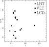 |
Fig. 1 U–I color vs. the observed I-band magnitudefor the AGNs studied in this work. Squares show the targets observed with FORS2 at the VLT telescope, triangles are the AGNs observed with MODS1-2 at the LBT telescope, while pentagons are the AGNs observed with the LDSS3 instrument at the Magellan-II Clay telescope. Three objects from Table 1 have no information on the U-band magnitude and are not plotted here. We do not plot COSMOS1710 since it is not at a redshift of ~ 4. |
2.2 Observations
We observed five objects with 22 hours of exposure in service mode with the MODS1-2 optical spectrographs at the LBT telescope and seven targets with FORS2 (with the blue enhanced CCDs) at the ESO VLT telescope, in 2 nights in visitor mode (Program 098.A-0862, PI A. Grazian). During several nights at the Magellan-II Clay telescope we observed four targets with the LDSS3 spectrograph, and we discovered one faint AGN at z ~ 4 during a pilot project. In total, we collected a sample of 16 relatively faint AGNs3 at 3.6 < z < 4.2, which is summarized in Table 1. The adopted exposure time per target varies according to the I band magnitudes and to the U–I colors of the AGNs.
AGN sample.
2.2.1 LBT MODS
During the observing period LBT2016 (Program 30; PI A. Grazian), we carried out deep UV spectroscopy of five faint AGNs (Fig. 1, triangles) down to an absolute magnitude M1450 = −24.0 (L ~ 2L*) at 3.6 < z < 4.2 with the LBT double spectrographs MODS1-2 (Pogge et al. 2012; Rothberg et al. 2016).
MODS is a unique instrument, since it is very efficient in the λobs ~ 4000 Å region, and it allows for observation of the whole optical spectrum, from λ ~ 3400 Å to ~ 10 000 Å, in a single exposure, which is essential for the goal of this paper. We have used MODS1-2, with the Blue (G400L) and Red (G670L) low-resolution gratings fed by the dichroic, reaching a resolution of R ~ 1000 for the adopted slit of 1.2 arcsec. The dispersion of the spectra is 0.5 Å/px for the G400L grating in the blue beam, and 0.8 Å/px for the G670L grating in the red beam, respectively.
The blue side of the MODS1-2 spectra was used to quantify the LyC escape fraction, sampling the spectral region blue-ward of 912 Å rest frame, while the red part (λ ~ 6000–10 000 Å) was used to fit the continuum at λrest ~ 1500–2000 Å of each AGN with a power law. The simultaneous observations of the blue and red spectra also allowed to get rid of variability effects which are affecting the escape fraction studies based on photometry taken in different epochs (e.g., Micheva et al. 2017). The simultaneous availability of the blue and the red spectra also allowed us to increase the survey speed by a factor of 2 with respect to traditional optical spectrographs on 8m class telescopes (i.e., FORS2 at VLT). Moreover, since the observations were executed in “Homogeneous Binocular” mode (i.e., with MODS1 and MODS2 pointing on the same position on the sky with the same configuration), by observing the same target with the two spectrographs, the survey speed gained another factor of 2, for a total net on-target time of 17 hours for five faint AGNs.
The LBT observations were executed in service mode by a dedicated team under the organization of the LBT INAF Coordination center. The average seeing during observations was around 1.0 arcsec, with airmass less than 1.3 and dark moon (≤ 7 days) in order to go deep in the UV side of the spectra.
The MODS1-2 spectrographs have been used in long slit spectroscopic mode, since our targets are sparse in the sky and do not fall on the same field of view. A dithering of ± 1.5 arcsec along the slit length was carried out in order to improve the sky subtraction and flat-fielding. The dithered observations were repeated several times, splitting each observation into sequences of 900 sec exposures.
The relative flux calibration was obtained by observing the spectro-photometric standard Feige34 for each observing night. The standard calibration frames (bias, flat, lamps for wavelength calibration) were obtained during day-time operation.
2.2.2 VLT FORS2
During the observing period ESO P98 (Program 098.A-0862; PI A. Grazian), we obtained deep FORS2 spectroscopy in visitor mode for seven faint AGNs (Fig. 1, squares) down to an absolute magnitude M1450 = −23.3 (L ~ L*). Two nights of VLT (21–22 of February, 2017) were assigned to our program. We used FORS2 with the blue optimized CCD in visitor mode. Among the VLT instruments, the blue optimized FORS2 is the only UV sensitive instrument that can be used for such scientific application. We adopted a slit width of 1.0 arcsec with the grism 300V (without the sorting order filter) which, coupled with the E2V blue optimized CCD, guarantees the maximum efficiency in the UV spectral region.
The typical seeing during observations was 0.6–1.4 arcsec, with partial thin clouds for the majority of the observing run. The adopted configuration allows us to cover the spectral window from 3400 to 8700 Å, centered at 5900 Å, with a dispersion of 3.4 Å/px and a resolution of R ~ 400. Exposure times ranged from 15 minutes to 2.2 hours, depending on the faintness of the targets and on their U–I color. Each observation was split in exposures of 1350 seconds, following an ABBA dithering pattern of ± 1.5 arcsec, in order to properly subtract the sky background and to carry out an accurate flat-fielding of the data.
At the beginning of the first night, the spectro-photometric standard star Hilt600 was observed in order to obtain a relative flux calibration of the targeted AGNs. All the remaining calibration frames (bias, flat, lamps for wavelength calibration) were obtained during day-time operations at the end of each observing night.
Three targets (SDSS04, SDSS20, SDSS27) were observed in long slit configuration, while the remaining AGNs (COSMOS955, COSMOS1311, COSMOS1710, COSMOS1782) were observed with multi object spectroscopy (MXU): in the COSMOS pointings, indeed, there are also many X-ray sources from Marchesi et al. (2016) and Civano et al. (2016) without spectroscopic identification. Given the legacy value of these targets, we carried out MXU observations in order to measure the redshifts of these fillers.
2.2.3 Magellan LDSS3
We used the LDSS3 spectrograph, mounted at the Magellan-II Clay 6.5m telescope at Las Campanas observatory (LCO), in February and March 2017 to observe four SDSS AGNs with I-band magnitude in the interval 21.0 ≤ I ≤ 21.5. We chose the grism VPH-Blue, with peak sensitivity around 6000 Å, wavelength coverage between 3800 and 6500 Å and a resolution R ~ 1400 for a slit of 1 arcsec width. The typical seeing during observations was 0.6–0.9 arcsec, matching the slit width of 1.0 arcsec. Each observation was split in exposures of 900 seconds, without any dithering pattern. The observations were taken under nonoptimal condition with respect to the lunar illumination, with a slightly high background in the UV. Moreover, the sensitivity of LDSS3 (equipped with red sensitive detectors) drops around 4000 Å rest frame, where the LyC of z ~ 4 sources is expected. For these reasons, we decided to observe relatively bright candidates in order to improve the number statistics by enlarging our sample.
In September 2017 a relatively faint AGN (UDS10275, I ~ 22.3) at z ~ 4.1 was serendipitously observed with the VPH-All grism and the LDSS3 instrument mounted at the Magellan-II Clay 6.5m telescope. The sensitivity of this grism peaks at λ = 7000 Å and covers the wavelength range between 4200 and 10 000 Å. While the sensitivity in the blue is slightly reduced with respect to the VPH-Blue grism, it allows for coverage of a larger spectral window, which is useful for the characterization of the properties of this target. With an exposure time of approximately 2 hours we were able to detect flux in the LyC region, as we discuss in detail in the following sections.
3 The method
3.1 Data reduction
The AGN spectra obtained with MODS1-2 were reduced by the INAF LBT Spectroscopic Reduction Center based in Milano4.
The LBT spectroscopic pipeline was developed inheriting the functionalities from the VIMOS pipeline (Scodeggio et al. 2005; Garilli et al. 2012), and was modified for the specific case of the dual MODS instruments. The pipeline corrects the science frames with basic pre-reduction (bias, flat field, wavelength calibration in two dimensions) and subtracts the sky from each frame by fitting the background with a polynomial function in two dimensions that takes into account the slit distortions. The relative flux calibration was carried out by computing the spectral response function thanks to the observations of the spectro-photometric standard star Feige34. Fully calibrated one-dimensional (1D) and two-dimensional (2D) extracted spectra with their associated RMS maps were produced at the end for each target, stacking all the available LBT observations after the cosmic ray rejection.
The FORS2 data were reduced with a custom software, developed on the basis of the MIDAS package (Warmels 1991). These tools are similar to the ones described in Vanzella et al. (2008). Briefly, the frames were pre-reduced with the bias subtraction and the flat fielding. For each slit, the sky background was estimated with a second order polynomial fitting. The sky fit was computed independently in each column within two free windows, above and below the position of the object. In the case of multiple exposures of the same source, the one dimensional spectra were co-added weighing according to the exposure time, the seeing condition and the resulting quality of each extraction process. Spatial median filtering was applied to each dithered exposure to eliminate the cosmic rays. Wavelength calibration was calculated on day-time arc calibration frames, using four arc lamps (He, HgCd, and two Ar lamps) providing sharp emission lines over the whole spectral range observed. The object spectra were then rebinned to a linear wavelength scale. Relative flux calibration was achieved by observations of the standard star Hiltner 600. For each reduced science spectrum we created also an RMS spectrum.
The data acquired with the LDSS3 instrument were reduced using the same custom package adopted to reduce the FORS2 data, deriving the relative flux calibrations through the spectro-photometric standard stars EG274 and LTT4816.
Figures 2–8, 9–13, and 14–18 show the AGN spectra obta- ined with FORS2 at VLT, MODS1-2 at LBT, and LDSS3 at Magellan telescope, respectively, as described in Table 1. In each spectrum, the blue region shows the spectral window covering LyC emission, that is, at λ ≤ 912 Å rest frame. The Magellan and LBT spectra were smoothed by a boxcar filter of 5 pixels for aesthetic reasons only, in order to match the spectral resolution with the effective resolution of the pictures.
3.2 Estimating the Lyman Continuum escape fraction of the faint AGNs
For each object in Table 1 the following measurements were carried out. First, we refine the input spectroscopic redshift by measuring the position of the OI 1305 emission line, which gives the systemic redshift. When this line is weak, we keep the original redshift  provided in Table 1, otherwisethe updated redshift
  can be found in Table 2. The exact determination of the systemic redshift for our AGNs is important since it allows us to measure precisely the position of the 912 Å break, and thus an accurate estimate of the LyC escape fraction for our objects. Only for the AGNs COSMOS1311 and SDSS04 have the spectroscopic redshifts been revised by small amounts, Δ z ~ 0.019 and − 0.004, respectively. The AGN COSMOS1710 instead had an incorrect spectroscopic redshift in Marchesi et al. (2016) and Civano et al. (2016) and was discarded in the following analysis.
After the refinement of the spectroscopic redshifts, we compute the LyC escape fraction for each AGN in our sample. We decided to adopt the technique outlined in Sargent et al. (1989) in order to measure fesc= exp(−τLL) from the spectra, where τLL is the opacity of the associated Lyman limit (LL). Precisely, we estimate the mean flux above and below the Lyman limit (912 Å rest frame) and measure the escape fraction as fesc = Fν(900)∕Fν(930), where Fν(900) is the mean flux of the AGN in the Lyman continuum region, namely between 892 and 905 Å rest frame, while Fν (930) is the average flux in the nonionizing region redward of the LL, between 915 and 945 Å rest frame, avoiding the region between 935 and 940 Å due to the presence of the Lyman-ϵ emission line. These average fluxes have been computed through an iterative clipping of spectral regions deviating more than 2σ from the mean flux values, as shown in Fig. 19 for AGN SDSS36. This method allows us to avoid spectral regions affected by some intervening strong IGM absorption systems or contaminated by emission lines. Similarly to Prochaska et al. (2009), we do not use the wavelength range close to the Lyman limit (905–912 Å rest frame) since it can be affected by the AGN proximity effect. In principle, the AGN proximity zone is a signature of ionizing photons escaping into the IGM, and should be considered in these calculation. However, we do not want to work too close to 912 Å rest frame in order to avoid biases due to possible incorrect estimates of the spectroscopic redshift. For this reason the LyC fesc provided in Table 2 should be considered as a robust lower limit for the real value.
This technique is different compared to the method adopted by Cristiani et al. (2016). They fit the SDSS QSO spectra with a power law in the wavelength range between 1284 and 2020 Å rest frame, avoiding the region affected by strong emission lines, and then extrapolate the fitted spectrum blueward of the Lyman-α line. After correcting for the spectral slope, they apply a mean correction for IGM absorption adopting the recipes of Inoue et al. (2014). Finally they computed the escape fraction as the mean flux between 865 and 885 Å rest frame, after normalizing the spectra to 1.0 redward of the Lyman-α. Since they apply an average correction for the IGM extinction, the LyC escape fraction of their bright QSOs goes from 0.0 to 2.5 (250%, see their Fig. 7). The values above 100% are simply due to the fact that in some QSOs the actual IGM absorption is lower than the mean value provided by Inoue et al. (2014). Since we do not want to rely on assumptions regarding the IGM properties surrounding our AGNs, we decided to adopt the technique of Sargent et al. (1989) outlined above, which gives a robust lower limit for the LyC escape fraction.
Finally we computed the absolute magnitude of our AGNs at 1450 Å rest frame starting from the observed I band magnitude in Table 1, M1450 = I–5 log10(DL) + 5 + 2.5log10(1 + zspec), where DL is the luminosity distance of the object and zspec is the refined spectroscopic redshift. At z ~ 4 the I band is sampling directly the 1450 Å rest frame, thus minimizing the K-correction effects.
Table 2 summarizes the measured properties (refined spectroscopic redshift, LyC escape fraction, absolute magnitude M1450) of the faint AGNs in our sample.
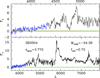 |
Fig. 2 Bottom: UV/optical spectrum of the AGN SDSS04 observed by FORS2 at VLT. Top: a zoom of the blue side of the spectrum for AGN SDSS04. The red horizontal lines mark the zero level for the flux Fλ, in arbitrary units. The LyC region (at λ ≤ 912 Å rest frame) has been highlighted in blue. The associated RMS is shown by the green spectrum. |
Measured properties of faint AGNs in our sample.
4 Results on the LyC escape fraction of high-z AGNs
The results summarized in Table 2 indicate that we detect a LyC escape fraction between 44% and 100% for all the 16 observed AGNs with absolute magnitude in the range − 25.14 ≤ M1450 ≤ −23.26. From a quantitative analysis of the spectra shown in Figs. 2–18, we confirm that the detection of HI ionizing fluxis significant for all the observed AGNs, with a signal-to-noise ratio (S/N) between 11 and 121 for our targets. Theuncertainties on the measured LyC escape fraction in Table 2 are of a few percent (~ 2–15%). The very good quality of these data is due to the usage of efficient spectrographs in the UV wavelengths and by the long exposure time dedicated tothis program (see Table 1). For the AGNs observed with the Magellan-II telescope the S/N is slightly lower, S∕N ~ 11–27, due to the nonoptimal conditions during the observations (high moon illumination).
With these spectra we confirm the detection of ionizing radiation for all 16 observed AGNs, with a mean LyC escape fraction of ~ 74% and a dispersion of ± 18% at 1σ level. The latter should not be considered as the uncertainty on the fesc measurements, but the typical scatter of the observed AGN sample.
4.1 Dependence of LyC escape fraction on AGN luminosity and U–I color
Figure 20 shows the dependence of the escape fraction on the absolute magnitude M1450 of the faint AGNs in our sample (filled triangles, squares, and pentagons). No particular trend with the absolute magnitude is observed in our data. In order to extend the baseline for the AGN luminosities, we adopt as reference the mean value of the escape fraction derived by Cristiani et al. (2016) for a sample of 1669 bright QSOs at z ~ 4 from the SDSS survey. They obtain a mean escape fraction of 75% for M1450 ≲−26, which is a luminosity approximately ten times larger than our faint limit M1450 ≤ −23.26. As is evident from Fig. 20, no trend of the escape fraction of ionizing photons with the luminosity of the AGNs/QSOs is detected. It is interesting to note that the quoted value for Cristiani et al. (2016) of M1450 ≲−26 represents the faint limit of the 1669 SDSS QSOs analysed, and their sample extends towards brighter limits M1450 ~ −29. Moreover, in Sargent et al. (1989) there are two QSOs (Q0000-263 and Q0055-264) with redshift z > 3.6 and absolute magnitudes of −29.0 and −30.2, with escape fraction close to 100%, and one QSO (Q2000-330) with M1450 = −29.8 and fesc ~ 70%. Finally, it is worth noting that the values of escape fraction provided in Table 2 are bona fide lower limits to the ionizing radiation, which can be even higher than 80% and possibly close to 100% if we take into account all the possible corrections (i.e., proximity effect, absorbers close to the LLS, intrinsic spectral slopes), as we discuss in Sect. 5.
The outcome of Fig. 20 is that the LyC escape fraction of QSOs and their fainter version (AGNs) does not vary in a wide luminosity range, between M1450 ~ −30 down to M1450 ~ −23, which is a factor of 103 in luminosity. More interestingly, we are reaching luminosities ≲ L* at z~ 4, which should provide the bulk of the emissivity at 1450 Å rest frame (Giallongo et al. 2012, 2015).
Figure 21 shows the LyC escape fraction of our faint AGNs versus the observed U–I color. No obvious trend is present, indicating that the typical color selection for z ~ 4 AGNs is not causing a notable effect on the LyC transmission for our sample.
The fact that we do not find any change in the properties of the escape fraction of faint AGNs (L ~ L*) with respect to the brighter QSO sample(L ~ 103L*) possibly indicates that even fainter AGNs (L ~ 10−2L*) at z~ 4 could have an escape fraction larger than 75% and possibly close to 100%. Although a gradual decrease of the escape fraction with decreasing luminosity would be expected by AGN feedback models (see e.g., Menci et al. 2008; Giallongo et al. 2012), this trend becomes milder as the redshift increases especially at z > 4. For this reason, in the following we assume that AGNs brighter than L ~ 10−2L* (M1450 ~ −18) have fesc ~ 75%. In a similarway, Cowie et al. (2009) and Stevans et al. (2014) show values of fesc close to unity both for bright QSOs and for much fainter Seyfert galaxies at lower redshifts. We use this assumption in the following sections to derive the contribution of the faint AGN population to the ionizing background at z ~ 4 and to make some speculations on the role of accreting super massive black holes (SMBHs) to the reionization process at higher redshifts.
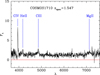 |
Fig. 8 UV spectrum of AGN COSMOS1710 observed by VLT FORS2. The spectroscopic redshift for this source in Marchesi et al. (2016) and Civano et al. (2016) turns out to be incorrect. The correct redshift is zspec = 1.547, thanks to many high-ionization lines detected in the spectrum (CIV, HeII, CIII, MgII, marked by the blue vertical lines). |
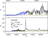 |
Fig. 9 Bottom: UV/optical spectrum of the AGN SDSS36 observed by MODS1-2 at LBT. Top: a zoom of the blue side of the spectrum for AGN SDSS36. The red horizontal lines mark the zero level for the flux Fλ, in arbitrary units. The LyC region (at λ ≤ 912 Å rest frame) has been highlighted in blue. The associated RMS is shown by the green spectrum. The scientific data have been smoothed by a boxcar filter of 5 pixels. |
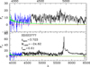 |
Fig. 14 Bottom: the whole spectrum of the AGN SDSS3777 observed by LDSS3 at Magellan. Top: a zoom of the blue side of the spectrum for AGN SDSS3777. The red horizontal lines mark the zero level for the flux Fλ, in arbitrary units. The LyC region (at λ ≤ 912 Å rest frame) has been highlighted in blue. The associated RMS is shown by the green spectrum. The scientific data have been smoothed by a boxcar filter of 5 pixels. |
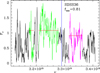 |
Fig. 19 Estimate of the LyC escape fraction for the AGN SDSS36 observed with MODS1-2 at the LBT telescope. The spectrum is in Fν and is arbitrarily normalized and blueshifted to z = 0 (rest-frame frequencies). The green portion of the spectrum shows the spectral region between 915 and 945 Å rest frame (excluding the wavelength range 935-940 Å due to the presence of the Lyman-ϵ emission line), while the magenta portion indicates the ionizing photons emitted between 892 and 905 Å rest frame. The blue vertical line indicates the location of the 912 Å rest-frame break. The red horizontal lines mark the mean values above and below the Lyman limit, after the iterative 2-σ clipping. The resulting escape fraction is the ratio between these two mean fluxes, and turns out to be 81% for SDSS36. |
4.2 The HI ionizing background at z ~ 4 produced by faint AGNs
In order to evaluate the contribution of faint AGNs to the HI ionizing background at z ~ 4 we assume that the LyC escape fraction is at least 75% for all the accreting SMBHs, from M1450 = −28 down to M1450 = −18, which corresponds approximately to a luminosity range 10−2L*≤ L ≤ 102L*, as carried out by Giallongo et al. (2015).
We use the same method adopted by Giallongo et al. (2015) to compute the UVB (in units of 10−12 photons per second, Γ−12) starting from the AGN luminosity function and assuming a mean free path of 37 proper Mpc at z = 4.0, in agreement with Worseck et al. (2014). To this aim, we adopt a spectral slope αν of –0.44 between 1200 and 1450 Å rest frame and –1.57 below 1200 Å rest frame, following Schirber & Bullock (2003). As discussed in Giallongo et al. (2015) and Cristiani et al. (2016), this choice is almost equivalent to assume a shallower slope of –1.41 below 1450 Å, as found by Shull et al. (2012) and Stevans et al. (2014).
In Table 3 we compute the value of the HI ionizing UVB Γ −12 assuming fesc (LyC) = 75% and considering different parameterizations of the z = 4 AGN luminosity function according to the different renditions found in the recent literature (Glikman et al. 2011; Giallongo et al. 2015; Akiyama et al. 2018; Parsa et al. 2018). When these luminosity functions are centered in a different redshift bin, we shift them to z = 4 applying a density evolution of a factor of 3 per unit redshift (i.e., 10−0.43z), according to the results provided by Fan et al. (2001) for the density evolution of bright QSOs. Here we assume that the bright and faint AGN populations evolve at the same rate, which may not be completely true (e.g., AGN downsizing, see Hasinger et al. 2005).
We provide the HI photo-ionization rate both at M1450 ≤ −23 and at M1450 ≤ −18. The values in parenthesis show the fraction of the UVB contributed by QSOs ad AGNs with respect to the value of Γ −12 = 0.85 found by (Becker & Bolton 2013, hereafter BB13) at z = 4. This value is required to keep the Universe ionized at these redshifts. If we adopt a UVB of Γ −12 = 0.55 found by Faucher-Giguère et al. (2008, hereafter FG08) at z = 4, then the fractional values in Table 3 should be increased by a factor of 1.55.
If we consider the contribution of QSOs and AGNs down to L ~L* (M1450 ≤ −23) we find an emissivity which is always 10–25% of the HI photo-ionization rate provided by BB13, irrespective of the adopted parameterization of the luminosity function. This fraction rises to 15–38% if the FG08 UVB is considered. Thus we can conclude, in agreement with Cristiani et al. (2016), that bright QSOs can provide 10–40% of the whole ionizing UVB at z ~ 4. This conclusion is robust with respect to the adopted UVB and for different parameterizations of the AGN luminosity function at these redshifts.
For fainter AGNs (M1450 ≤ −18) the situation depends critically on the adopted luminosity function at z ~ 4 and on the exact value of the HI photo-ionization rate measured through the Lyman-α forest statistics. Assuming a UVB by BB13, then the contribution of faint AGNs is between 16 and 73%, adopting the luminosity function of Akiyama et al. (2018) and Giallongo et al. (2015), respectively. It is worth noting here that there are still large uncertainties on the observed space density of L ~L* AGNs at z ≥ 4 and that the luminosity function of Akiyama et al. (2018) is systematically lower, by a factor of ten, than the one of Glikman et al. (2011) at M1450 ~ −23 (see Fig. 18 of Akiyama et al. 2018). While the result of Glikman et al. (2011) can be considered as a lower limit for the space density of QSOs at z ~ 4, since it has been derived from a spectroscopically complete sample of point-like type-1 QSOs only, it could be affected by large uncertainties related to the completeness corrections. For these reasons, a firm value of the luminosity function at M1450 ~ −23 is still required.
Recently, Parsa et al. (2018) revised the results of Giallongo et al. (2015), deriving a different parameterization for the luminosity function at z ≥ 4. It should be noted, however, that the space density at M1450 ≥−21 in Parsa et al. (2018) at z = 4.25 is similar to the one by Giallongo et al. (2015). Their contribution to the UVB is significantly lower than Giallongo et al. (2015) since they adopt a rather flat luminosity function, with a normalization around the break (M1450 ~ −23) which is significantly lower than the space density provided both by Giallongo et al. (2015) and by Glikman et al. (2011). As discussed extensively in Giallongo et al. (2012, 2015), the bulk of the ionizing UVB comes directly from objects close to the break of the luminosity function, thus exactly where the Parsa et al. (2018) fit is below the observed number density of AGNs by Glikman et al. (2011). It is thus not surprising that their luminosity function is providing only 30% of the HI photo-ionization rate at z = 4.
Summarizing, the faint AGN population at z ~ 4 are able to contribute, adopting the Glikman et al. (2011) and Giallongo et al. (2015) luminosity functions, respectively, to 36–73% of the UVB, assuming the BB13 determination, or 56–100% of the UVB, assuming FG08 measurement, as shown in Fig. 22. If the luminosity functions of Akiyama et al. (2018) or Parsa et al. (2018) are adopted, instead, the faint AGN population is able to provide only 16–30% of the BB13 UVB, or 25–47% of the FG08 UVB, respectively. Our conclusion is that, taking into account the uncertainties on the UVB determination and the knowledge of the z ~ 4 AGN luminosity function, the population of accreting SMBHs at these redshifts can contribute to a non-negligible fraction of the HI photo-ionization rate. They can provide at least 16% of the UVB in the most conservative case, adopting the Akiyama et al. (2018) or Parsa et al. (2018) luminosity functions, but this can reach 100% if the space density of L ~ L* AGNs is comparable to that found by Glikman et al. (2011) or Giallongo et al. (2015). This result is based on the extrapolation that the LyC escape fraction of AGNs remains constant at approximately the 75% level down to M1450 ~ −18. This assumption is not unreasonable, according to Fig. 20, and should be checked with future observations.
This result is fundamental to deciphering whether or not faint AGNs are the main drivers of the reionization epoch at z > 6, under the reasonable assumptions that the LyC fesc remains roughly constant from z ~ 4 to z ≥ 6 and that the space density of faint AGNs is of the order of that found by Giallongo et al. (2015) up to z ~ 6. This conclusion will hold if we assume that the physical properties of AGNs do not vary dramatically from z = 4 to z ≥ 6. Given the similarity in the optical-UV spectra of faint AGNs in the local Universe (Stevans et al. 2014) and bright QSOs at z ≥ 4 (Prochaska et al. 2009; Worseck et al. 2014; Cristiani et al. 2016), this assumption can be considered safe.
In addition, we can use the estimation of the UV background by faint AGNs at z = 4 provided in Table 3 to derive a reasonable upper limit to the relative escape fraction of the star-forming galaxy population at this redshift. Assuming for example the HI ionizing background of BB13 and the AGN Luminosity Function of Glikman et al. (2011), a relative escape fraction of 4.8% for the galaxy population5 should be assumed in order to complement the AGN contribution to Γ −12. Alternatively, an escape fraction of ~2% for the galaxy population is needed to complement the AGN contribution if a luminosity function by Giallongo et al. (2015) is assumed for AGNs atz ~ 4, or if we adopt the Glikman et al. (2011) luminosity function but considering the UV background by FG08. Finally, if we consider the luminosity function by Giallongo et al. (2015) and the UVB by FG08, then all the HI ionizing background is produced by AGNs and the upper limit to the escape fraction for galaxies is close to zero. If confirmed, these upper limits we have obtained at z = 4 for star-forming galaxies, that is, fesc,rel of 0–5%, are comparable to the values found at lower redshifts (e.g., Grazian et al. 2016, 2017), indicating amild evolution in redshift of the LyC escape fraction for star-forming galaxies at z ≲ 4. For comparison, Cristiani et al. (2016) find a slightly higher value of 5.5-7.6% for the LyC escape fraction of z ≥ 4 galaxies. Without a significant change in this trend at higher redshifts, it would be difficult for the galaxy population to reach values of fesc,rel ~ 15%, required in order to reach reionization at z ~ 7 with stellar radiation only (Madau 2017). At high z there are however indications that the LyC photon production efficiency ξion could be larger than the estimates at z≤ 2 (Bouwens et al. 2016), thus slightlyrelaxing the fesc,rel ~ 15% requirement. Moreover, the star-forming galaxy luminosity function steepens at higher redshifts (e.g., Finkelstein et al. 2015) further relaxing the constraint on the galactic LyC escape fraction. Considering the large uncertainties on the faint-end slope and on the possible cut-off (at M1500 ~ −13, see e.g., Livermore et al. 2017 and Bouwens et al. 2017) of the luminosity function, an escape fraction of ~ 4–11% (assuming ξion = 1025.3) can still be sufficient for star-forming galaxies to keep the Universe ionized at z > 5 (Madau 2017).
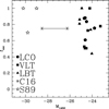 |
Fig. 20 Dependence of the LyC escape fraction on the absolute magnitude M1450 for QSOs and AGNs at 3.6 ≤ z ≤ 4.2. Squares show the targets observed with the VLT telescope, triangles are the AGNs observed with MODS1–2 at the LBT telescope, while pentagons are the AGNs observed with the LDSS3 instrument at the Magellan-II Clay telescope. The uncertainties on the measured LyC escape fraction at M1450 ≳−25 are of a few percent (~2–15%). The two asterisks connected by an horizontal line show the range of M1450 for the QSOs studied by Cristiani et al. (2016), while the three stars are three very bright QSOs (M1450 ~ −30) studied by Sargent et al. (1989, S89). No obvious trend of fesc with the absolute magnitude M1450 is detected. |
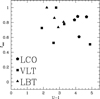 |
Fig. 21 Dependence of LyC escape fraction on the observed U–I color for our faint AGNs. No obvious trend has been detected. Three objects from Table 1 have no information on the U-band magnitude and are not plotted here. |
HI photo-ionization rate Γ−12 produced by AGN at z ~ 4.
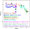 |
Fig. 22 HI photo-ionization rate measured by different estimators from the literature as a function of redshift. The magenta square shows the estimated value for the emissivity of AGNs at z ~ 4, assuming a luminosity function of Giallongo et al. (2015) down to M1450 = −18. The gray square indicates the contribution of faint AGNs adopting a luminosity function of Glikman et al. (2011). The green and violet squares indicate the AGN emissivity assuming a luminosity function of Parsa et al. (2018) and Akiyama et al. (2018), respectively. A LyC escape fraction of 75% has been assumed. The UVB derived by FG08 has been shown with filled blue circles, while we represent with open blue circles the same data of FG08 rescaled with a different temperature-density relation, as described in Calverley et al. (2011). |
5 Discussions
5.1 Target selection
The extension of our results to the whole AGN population at z ~ 4 depends critically on the sample adopted to carry out the LyC escape fraction measurement. The ideal sample should be an unbiased subsample of all the AGNs (both obscured and unobscured), without any biases against or in favor of strong LyC emission. Our starting sample is a mix of optically- and X-ray-selected AGNs from SDSS3-BOSS (Dawson et al. 2013), from the NDWFS/DLS survey (Glikman et al. 2011), and from Chandra X-ray observations in the COSMOS field (Marchesi et al. 2016; Civano et al. 2016), selected only in redshift (3.6< z < 4.2) and in I-band apparent magnitude (21 < I < 23).
The SDSS has searched for high-z QSOs adopting optical color criteria based on dropouts, and thus this selection is not biased in favor of strong LyC emitters, but could be biased against them. A large value for fesc (LyC) indeed would reduce the drop-out color used to select high-z sources. As shown in Prochaska et al. (2009), the selection of z ≤ 3.6 QSOs in the SDSS-DR7 (Abazajian et al. 2009) is instead biased against blue (u − g < 1.5) objects, that is, they are prone to select sightlines with strong Lyman limit absorptions, active nuclei with strong emission lines or low escape fraction.
On the other hand, the X-ray selection is not biased towards obscured AGNs, but in our sample only four objects (25%) have been selected through this criterion. We do not find any difference between the properties of X-ray and optically selected AGNs in our sample. In the future, the exploitation of a complete X-ray-selected sample of (both obscured and unobscured) faint AGNs will be instrumental to check whether or not type-2 AGNs emit LyC photons (Cowie et al. 2009 find that they do not radiate ionizing photons) and to put firmer constraints on the global emissivity of the whole population of accreting SMBHs at high z.
In summary, our sample is representative of the whole AGN population at L ~ L*, and is not biased against or in favor of strong LyC emitters, as shown in Figs. 1 and 21.
5.2 The fraction of BAL AGNs
Active galactic nuclei that show strong absorption features in the Lyman-α line, a population called BAL QSOs, have been excluded from our sample. The large column density (NHI ≥ 1019cm−2) associated to the strong absorbing systems could imply a complete suppression of the flux in the LyC region.
Allen et al. (2011) and Pâris et al. (2014) have estimated the BAL fraction of bright QSOs in the SDSS to be around 10–14%. In principle this particular class of AGNs should be included in our sample in order to obtain an estimate of the ionizing contribution of the whole AGN population, as done by Cristiani et al. (2016). However, it has not yet been established whether all the BAL population has negligible emission of LyC photons. As an example, in the lensed BAL QSO APM08279+5255 at z = 3.9, significant emission has been detected in the LyC region (see Fig. 1 of Saturni et al. 2016).
Moreover, McGraw et al. (2017) show the relevant examples of appearing and disappearing broad absorptions in SDSS QSOs at z ~ 2–5 on timescales of one to five rest-frame years for 2–4% of the observed BAL sample. A possible explanation of the BAL variability over multi-year timescales implies changes in either the gas ionisation level or in the covering factor, supporting transverse-motion and/or ionization-change scenarios to explain BAL variations. This indicates that it is a relatively fast phenomenon, which is probably due to the small-scale environment of the accreting SMBH (few kpc), and it is probably not affecting its isotropic emission of ionizing photons on cosmological timescales related to the QSO lifetime or on cosmological scales (Mpc).
For these reasons, we decided not to correct the value of LyC fesc found with our sample for the fraction of BAL QSOs present in the global population of AGNs. In the future, a systematic study of the LyC escape fraction and of the fraction of BAL objects at different luminosities will be important to assess the total contribution of the whole AGN population to the ionizing UVB.
5.3 Reliability of LyC fesc measurement
The uncertainties related to the LyC escape fraction measurements described above mainly depend on the S/N of the spectra and on the determination of the systemic redshift of the AGN, which can be obtained through the position of the OI 1305 emission line. In our case, only for two AGNs (COSMOS1311 and SDSS04) do we have good quality spectra that allow us to refine the spectroscopic redshifts. For the other AGNs, we rely on the published spectroscopic redshifts.
The shift in redshift applied to COSMOS1311 and SDSS04 is not affecting our LyC fesc estimate. To avoid mismatch for the position of the LyC region, we decided to measure the escape fraction relatively far from the LyC break, i.e., between 892 and 905 Å rest frame. For example, considering the Δ z ~ 0.019 correction for COSMOS1311, it will move the 905 Å rest-frame wavelength to 908 Å. In the unlikely case that the adopted shift is not correct, we are still estimating the escape fraction in the LyC region. In general, since the corrections to the observed redshifts for our sample are low, we are not biasing our estimates towards higher values of LyC fesc for our AGNs.
The S/N of our spectra in the LyC region varies between 11 and 121, when integrated between 892 and 905 Å rest frame and along the slit. This translates to an uncertainty on the measured LyC escape fraction of a few percent (~ 2–15%). This shows that our measurements of the ionizing emissivity of faint AGNs are robust against statistical and systematic errors.
We assume here that the contribution of the intrinsic slope of the AGN has negligible impact on the flux ratio between 900 and 930 Å rest frame, since this wavelength interval is relatively limited. Since the typical spectral slope of AGNs is Fν ∝ ναν with αν approximately between –0.5 and –1.0, it turns out that the impact on the LyC escape fraction estimate is to decrease the observed LyC fesc with respect to the true one. Correcting, for example, for the intrinsic spectral slope of AGN, indeed, provides only a negligible correction of the order of 2%, assuming, for example, αν = −0.7.
We have also avoided the region within the Stromgreen sphere of the AGN itself, the so-called proximity region. If part of the proximity region is included in our calculations, i.e., measuring the ionizing radiation between 892 and 910 Å rest frame instead of limiting to 905 Å, we obtain an escape fraction which is on average 4% higher for our 16 AGNs, but with large scatter from object to object. As can be seen from Figs. 2 and 9, the IGM absorption can vary greatly from different lines of sight, and in some cases it turns out that the proximity region between 905 and 910 Å are affected by intervening absorbers (e.g., at λ ~ 907 Å rest frame for SDSS36 in Fig. 19).
Indeed, if we correct our estimate of the escape fraction for the flux decrement due to intervening absorbing systems between 930 and 900 Å rest frame, adopting, for example, Inoue et al. (2014) at z = 4 or Prochaska et al. (2009) at z = 3.9, we obtain a corrected LyC escape fraction which is close to 100%. This indicates that our method provides a conservative lower limit to the LyC escape fraction of faint AGNs, and there are robust indications that the corrected estimate could be close to fesc = 100% for our objects.
5.4 The LyC escape fraction of low-luminosity AGNs
There are two different aspects of the problem on the sources of ionizing photons. Are the LyC photons emitted by stars or are they the result of accretion onto SMBHs? And are the ionizing photons able to escape into the IGM as the result of stellar feedback (winds, SNe), or as the result of AGN energetic feedback into the ISM? We can try to derive some clues here. If the carving of free channels in the ISM of a galaxy has been driven by a ubiquitous mechanism such as supernovae or stellar winds, then we can expect that a significant LyC escape fraction must be a common and widespread phenomenon among SFGs. Since this is not the case (e.g., Grazian et al. 2016, 2017; Japelj et al. 2017), and Lyman-continuum emitters are rare and peculiar cases both in the local Universe and at high z (e.g., Izotov et al. 2016a,b; de Barros et al. 2016; Vanzella et al. 2016; Shapley et al. 2016; Bian et al. 2017), we can probably exclude a scenario where the cleaning of free paths in the galaxies ISM is due to SNe or stellar wind; it could, however, be caused by rarer phenomena like accreting BHs, such as AGNs or X-ray binaries (XRBs).
At this point, it is important to explore the dependencies of the LyC escape fraction on the luminosities of the AGNs. Interestingly, Kaaret et al. (2017) find that the Lyman-continuum-emitting galaxy Tol 1247–232 (fesc,rel = 21.6%, Leitherer et al. 2016; see, however, Puschnig et al. 2017 for a lower estimate) has been detected in X-ray as a point-like source by Chandra, and it shows also X-ray variability by a factor of two in a few years, thus is probably a low-luminosity AGN (Lx ~ 1041 erg s−1) at z = 0.048. Another LyC source, Haro 11, with fesc,abs ~ 3% (Leitet et al. 2011), has been detected in X-ray as abright point source with a very hard spectrum (Prestwich et al. 2015). In addition to these two galaxies, Borthakur et al. (2014) show an example of a LyC emitter (J0921+4509, fesc,abs ~ 20%), which has been detected in hard X-rays by XMM (Jia et al. 2011), possibly revealing its AGN nature.
We can link our observations at z ~ 4 with the results by Kaaret et al. (2017) for extremely faint AGNs in the local Universe. The LyC escape fraction of AGNs with Lx = 1044 erg s−1 is substantial (~ 80–100%) at 0≤ z ≤ 4 as shown by this work and by the recent literature (Cowie et al. 2009; Stevans et al. 2014; Prochaska et al. 2009; Cristiani et al. 2016), while it is only a few percent for the two faint AGNs of Kaaret et al. (2017), with Lx = 1041 erg s−1 at z ~ 0. As we show in the following, this is not in contrast with our conclusions above.
The total UV absolute magnitudes of Tol 1247-232 and Haro 11 are ~ − 20∕–21, which translate into effective magnitudes of ~ −15∕–16 at 900 Å rest frame, given the observed values for their LyC escape fraction. Starting from the X-ray luminosity of Lx ~ 1041 erg s−1 measured by Kaaret et al. (2017) for their central sources, and assuming that the optical luminosities are scaling as  (Lusso & Risaliti 2016), we derive an absolute magnitude of M1450 ~ −12 for the central AGNs in Tol 1247–232 and Haro 11. This implies that the ionizing radiation by these two galaxies cannot be entirely produced by the central engines, even assuming an escape fraction of 100% for the central AGN, but it is possibly emitted also by the surrounding stars, once the AGN has cleaned the surrounding ISM. As a consequence, a large mechanical power, probably available only in accreting SMBHs, can drive the emission of copious amounts of ionizing photons, even in very-low-mass or low-luminosity galaxies, as suggested by theoretical models (Menci et al. 2008; Giallongo et al. 2012; Dashyan et al. 2018) and seen in observations (e.g., Penny et al. 2018). If a linear relation between Lx and Lopt were instead adopted for these two AGNs, then their magnitudes would be M1450 ~ −15∕–16. In this case, it would possible for the ionizing flux to be entirely provided by the central AGN, with an effective escape fraction ~ 50–100%, indicating a relatively mild evolution of fesc with the AGN luminosity over a very broad range of absolute magnitudes.
Moreover, it is worth pointing out that the two galaxies studied by Kaaret et al. (2017) lie within the pure star-forming region of the Baldwin-Phillips-Terlevich (BPT, Baldwin et al. 1981) diagram and that there are no indications for the presence of an active nucleus at other wavelengths (Leitet et al. 2013). For this reason, these objects have not been considered in the AGN population in the previous studies, which are thus underestimating the correct space density of accreting SMBHs at faint luminosities. Interestingly, these peculiar sources are not taken into account when one investigates the AGN contribution to the ionizing UVB. This point is also corroborated by the results of Cimatti et al. (2013) and Talia et al. (2017), who showed that there are AGNs at z > 2 which are not showing any kind of nuclear activity signature in their optical spectra. In the local Universe, Chen et al. (2017) concluded that 30% of the AGNs observed by NuSTAR are not detected in soft X-ray, Optical, or IR, thus evading the typical AGN selection criteria. In the future, a detailed and complete census of the whole AGN population at high redshifts and at faint luminosities will allow a better understanding of the reionization process.
5.5 The issue of an overly high IGM temperature with an AGN dominating HeII reionization
A scenario where HI reionization is driven mainly by AGNs has the draw back of heating the IGM to an overly high temperature at the epoch of HeII reionization, which is foreseen at z ~ 4 (Worseck et al. 2016). Such an issue is present in models of AGNs dominating both HI and HeII reionizations, as discussedin D’Aloisio et al. (2017, 2018). Their simulations show that an AGN-dominated model is in tension with the available constraints on the thermal history of the IGM, since the early HeII reionization at z ~ 4 is heating up the IGM at a temperature T ~ 2 × 10⁴ K, well above the Lyman-α forest temperature of T ~ 104 K, inferred by Becker et al. (2011) through the comparison with hydrodynamic simulations.
Recently, Puchwein et al. (2018) drew a similar conclusion, that is, that models with a large AGN contribution to the high-z UVB are disfavored by the low IGM temperature determination of Becker et al. (2011). It is worth pointing out, however, that measuring the IGM temperature from the Lyman-α forest opacity is very challenging. At present, the existing measurements of TIGM show a large variance, with differences of even a factor of 2–2.5 between different methods (TIGM ~ 104–2.5 × 10⁴K at z ≥ 3; see, for example, Puchwein et al. 2018; Hiss et al. 2017; Garzilli et al. 2012; Lidz et al. 2010). Clearly, more observations and detailed simulations are needed in order to understand the origin of these discrepancies. Given the large uncertainties that are still present on the determination of the IGM temperature at z ≥ 3, a scenario where AGNs give a significant contribution to the reionization cannot be ruled out.
Moreover, it is also possible that the extreme UV spectra of low-luminosity AGNs are softer than those of bright QSOs, due to the contribution of the host galaxy to the escaping LyC photons, once the active SMBH has opened a clear path into the ISM. As a consequence, the impact of low-luminosity AGNs and their host galaxies on the HeII reionization could be in better agreement with the predictions of D’Aloisio et al. (2017, 2018) and Puchwein et al. (2018).
5.6 Future activities
In this paper we have shown that z ~ 4 AGNs with L ≳ L* have in general a large escape fraction of HI ionizing photons, and can contribute to ≥ 50% of the UVB at these redshifts. With the present data, it is not possible to make strong conclusions on whether or not AGNs are the main drivers of the HI reionization at z > 6, since their number densities are still uncertain at z ≥ 4 (Giallongo et al. 2015; Ricci et al. 2017; Parsa et al. 2018; Matsuoka et al. 2018; Onoue et al. 2017).
In order to gain further insight into this important open question, three major advances are required in the field of high-z AGNs: (1) it is crucial at this point to confirm or disprove with large number statistics and at fainter luminosities (L ≤ L*) the result found in this paper, i.e., that faint AGNs have a substantial LyC escape fraction (fesc ~ 75%), similarly to very bright high-z QSOs; (2) the luminosity function at z ≥ 4 is still poorly sampled, especially around L ~ 0.1–1.0 L*, where the bulk of ionizing photons is expected; and (3) the current measurements of the photo-ionization rate Γ −12 at z > 2 are still uncertain (e.g., FG08 vs. BB13), as discussed in the previous section. These are three fundamental steps to understanding whether faint AGNs are the potential drivers of the reionization process. In this paper we have begun to answer the questions summarized in point (1), that is, the escape fraction of faint AGNs. In a future paper we will explore the dependencies of the LyC escape fraction on the physical properties of our faint AGN sample at z ~ 4. In Giallongo et al. (in prep.) we are investigating the luminosity function of AGNs at z ≥ 4 at M1450 ≥−21. In order to provide precise answers to point (2), however, a dedicated survey of L ~0.1–1.0 L* AGNs (bothof type-1 and type-2) is required. The exact determination of the ionizing UVB has been discussed extensively by many authors. It is not trivial to directly translate the observations of the Lyman forest opacity of high-z QSOs into an estimate of the UVB. For example, BB13 explore the differences between their UVB determination and that of FG08. They ascribe the discrepancy to the assumed temperature-density relation (due primarily to their lower IGM temperatures) and to the effect of peculiar velocities and thermal broadening. In the future, detailed simulations of the IGM at high spatial resolution will probably be able to address these issues in more detail.
6 Summary and conclusions
Most papers related to the hydrogen reionization at high-z state that star-forming galaxies are the most obvious and natural mechanism for producing the required ionizing photons. An alternative scenario is possible, i.e., that faint AGNs could provide a great fraction of the HI ionizing UVB, at least at z ~ 4. This has important implications for the role of galaxies and AGNs in the reionization of the Universe.
We selected 16 AGNs at z ~ 4 in a magnitude range − 25.1 ≲ M1450 ≲−23.3 (i.e., L*≲ L ≲ 7L*) with the aim of measuring the LyC escape fraction of a representative sample of relatively faint AGNs. We have shown that with typical exposure times of texp ~ 2–6 hours per target at six to eight-metre-class telescopes, equipped with UV sensitive instruments (e.g., FORS2 and MODS1–2), the quality of the acquired spectra is high enough to study the LyC emission of L ~ L* AGNs. Our limited sample is already suggesting a relatively large escape fraction of HI ionizing photons (fesc ≥ 75%) for the whole AGN population with L ≳ L* at a very high confidence level (S∕N ~ 10–120). Therefore, the ionizing properties of the faint AGN population at z ~ 4 are similar to those of the brightest QSOs, that is, M1450 ~ −30 or L ~ 103L*, at the same redshift.
Assuming the luminosity functions of Glikman et al. (2011) or Giallongo et al. (2015) at z ~ 4, and extrapolating the AGN contribution down to a magnitude of M1450 ~ −18, AGNs can provide between 36 and 73% of the UVB measured by BB13. If the UVB by FG08 is considered instead, the integrated AGN contribution rises up to 56–100%. Adopting other luminosity functions (e.g., Parsa et al. 2018; Akiyama et al. 2018) gives a lower contribution (16–30% of the ionizing UVB measured by BB13).
Based on these results, we conclude that faint (L ~ L*) AGNs could provide a crucial contribution to the cosmological UV background up to z = 4, and, if the large escape fraction and high space densities for AGNs are confirmed also at z ~ 5–7, they could be responsible for the reionization of the Universe. This result is in agreement with recent models showing that a large contribution from AGNs to the ionizing background is sufficient to account for the observed probability distribution function of the opacity τGP in the lines of sight of bright z ~ 6 QSOs (Chardin et al. 2015, 2017). D’Aloisio et al. (2017) reach a similar conclusion, though finding that an AGN-driven reionization scenario heats the IGM to overly high temperatures at the epoch of HeII reionization. It is worth mentioning that the present measurements of the IGM temperature at z > 3 are characterized by large variance, due to the difficulties in comparing Lyman-α forest opacity observations and simulations (e.g., Hiss et al. 2017; Puchwein et al. 2018).
In the future, it will be possible to substantiate these conclusions by extending the present analysis on the LyC escape fraction of AGNs to fainter luminosities (L < L*) and to the BAL class, by measuring with high accuracy the AGN space density near the break (M1450 ~ −23) of the luminosity function at z ≥ 4. Further evidence will also be provided by estimating, in an unbiased and possibly direct way, the ionizing UVB at z ≥ 4 and the IGM temperature.
Acknowledgements
We warmly thank the anonymous referee for her/his useful suggestions and constructive comments that help us to improve this paper. AG and EG warmly thank Piero Madau and Enrico Garaldi for useful discussions. The LBT is an international collaboration among institutions in the United States, Italy, and Germany. LBT Corporation partners areThe University of Arizona on behalf of the Arizona university system; Istituto Nazionale di Astrofisica, Italy; LBT Beteiligungsgesellschaft, Germany, representing the Max-Planck Society, the Astrophysical Institute Potsdam, and Heidelberg University; The Ohio State University; and The Research Corporation, on behalf of The University of Notre Dame, University of Minnesota, and University of Virginia. This paper used data obtained with the MODS spectrographs built with funding from NSF grant AST-9987045 and the NSF Telescope System Instrumentation Program (TSIP), with additional funds from the Ohio Board of Regents and the Ohio State University Office of Research. Based on observations collected at the European Organisation for Astronomical Research in the Southern Hemisphere under ESO programme 098.A-0862.
References
- Abazajian, K. N., Adelman-McCarthy, J. K., Agüeros, M. A., et al. 2009, ApJS, 182, 543 [NASA ADS] [CrossRef] [Google Scholar]
- Akiyama, M., He, W., Ikeda, H., et al. 2018, PASJ, 70, S34 [NASA ADS] [CrossRef] [Google Scholar]
- Allen, J. T., Hewett, P. C., Maddox, N., Richards, G. T., & Belokurov, V. 2011, MNRAS, 410, 860 [NASA ADS] [CrossRef] [Google Scholar]
- Baldwin, J. A., Phillips, M. M., & Terlevich, R. 1981, PASP, 93, 5 [NASA ADS] [CrossRef] [EDP Sciences] [Google Scholar]
- Becker, G. D., & Bolton, J. S. 2013, MNRAS, 436, 1023 [NASA ADS] [CrossRef] [Google Scholar]
- Becker, G. D., Bolton, J. S., Haehnelt, M. G., & Sargent, W. L. W. 2011, MNRAS, 410, 1096 [NASA ADS] [CrossRef] [Google Scholar]
- Becker, G. D., Bolton, J. S., Madau, P., et al. 2015, MNRAS, 447, 3402 [NASA ADS] [CrossRef] [Google Scholar]
- Bian, F., Fan, X., McGreer, I., et al. 2017, ApJ, 837, L12 [NASA ADS] [CrossRef] [Google Scholar]
- Bolton, J. S., Haehnelt, M. G., Viel, M., & Springel, V. 2005, MNRAS, 357, 1178 [NASA ADS] [CrossRef] [Google Scholar]
- Borthakur, S., Heckman, T. M., Leitherer, C., & Overzier, R. A. 2014, Science, 346, 216 [NASA ADS] [CrossRef] [Google Scholar]
- Bouwens, R. J., Illingworth, G. D., Oesch, P. A., et al. 2015, ApJ, 803, 34 [NASA ADS] [CrossRef] [Google Scholar]
- Bouwens, R. J., Smit, R., Labbé, I., et al. 2016, ApJ, 831, 176 [NASA ADS] [CrossRef] [Google Scholar]
- Bouwens, R. J., Oesch, P. A., Illingworth, G. D., Ellis, R. S., & Stefanon, M. 2017, ApJ, 843, 129 [NASA ADS] [CrossRef] [Google Scholar]
- Bridge, C. R., Teplitz, H. I., Siana, B., et al. 2010, ApJ, 720, 465 [NASA ADS] [CrossRef] [Google Scholar]
- Calverley, A. P., Becker, G. D., Haehnelt, M. G., & Bolton, J. S. 2011, MNRAS, 412, 2543 [NASA ADS] [CrossRef] [Google Scholar]
- Chen, C.-T. J., Brandt, W. N., Reines, A. E., et al. 2017, ApJ, 837, 48 [NASA ADS] [CrossRef] [Google Scholar]
- Cimatti, A., Brusa, M., Talia, M., et al. 2013, ApJ, 779, L13 [NASA ADS] [CrossRef] [Google Scholar]
- Chardin, J., Haehnelt, M. G., Aubert, D. & Puchwein, E. 2015, MNRAS, 453, 2943 [NASA ADS] [CrossRef] [Google Scholar]
- Chardin, J., Puchwein, E., & Haehnelt, M. G. 2017, MNRAS, 465, 3429 [NASA ADS] [CrossRef] [Google Scholar]
- Civano, F., Marchesi, S., Comastri, A., et al. 2016, ApJ, 819, 62 [NASA ADS] [CrossRef] [Google Scholar]
- Cowie, L. L., Barger, A. J., & Trouille, L. 2009, ApJ, 692, 1476 [NASA ADS] [CrossRef] [Google Scholar]
- Cristiani, S., Serrano, L. M., Fontanot, F., Vanzella, E., & Monaco, P. 2016, MNRAS, 462, 2478 [NASA ADS] [CrossRef] [Google Scholar]
- D’Aloisio, A., Upton Sanderbeck, P. R., McQuinn, M., Trac, H., & Shapiro, P. R. 2017, MNRAS, 468, 4691 [NASA ADS] [CrossRef] [Google Scholar]
- D’Aloisio, A., McQuinn, M., Davies, F. B., & Furlanetto, S. R. 2018, MNRAS, 473, 560 [NASA ADS] [CrossRef] [Google Scholar]
- Dashyan, G., Silk, J., Mamon, G. A., Dubois, Y, & Hartwig, T. 2018, MNRAS, 473, 5698 [NASA ADS] [CrossRef] [Google Scholar]
- Davies, F. B., Hennawi, J. F., Eilers, A.-C., & Lukić, Z. 2017, ApJ, 855, 106 [Google Scholar]
- Dawson, K. S., Schlegel, D. J., Ahn, C. P., et al. 2013, AJ, 145, 10 [Google Scholar]
- de Barros, S., Vanzella, E., Amorín, R., et al. 2016, A&A, 585, A51 [NASA ADS] [CrossRef] [EDP Sciences] [Google Scholar]
- Drake, A. B., Garel, T., Wisotzki, L., et al. 2017, A&A, 608, A6 [NASA ADS] [CrossRef] [EDP Sciences] [Google Scholar]
- Fan, X., Strauss, M. A., Schneider, D. P., et al. 2001, AJ, 121, 54 [NASA ADS] [CrossRef] [Google Scholar]
- Fan, X., Strauss, M. A., Becker, R. H., et al. 2006, AJ, 132, 117 [NASA ADS] [CrossRef] [EDP Sciences] [Google Scholar]
- Faucher-Giguère, C.-A., Lidz, A., Hernquist, L. & Zaldarriaga, M. 2008, ApJ, 688, 85 [NASA ADS] [CrossRef] [Google Scholar]
- Finkelstein, S. L., Papovich, C., Ryan, R. E., et al. 2012, ApJ, 758, 93 [NASA ADS] [CrossRef] [Google Scholar]
- Finkelstein, S. L., Ryan, R. E. Jr., Papovich, C., et al. 2015, ApJ, 810, 71 [NASA ADS] [CrossRef] [Google Scholar]
- Fontanot, F., Cristiani, S. & Vanzella, E. 2012, MNRAS, 425, 1413 [NASA ADS] [CrossRef] [Google Scholar]
- Garilli, B., Paioro, L., Scodeggio, M., et al. 2012, PASP, 124, 1232 [NASA ADS] [CrossRef] [Google Scholar]
- Garzilli, A., Bolton, J. S., Kim, T.-S., Leach, S., & Viel, M. 2012, MNRAS, 424, 1723 [NASA ADS] [CrossRef] [Google Scholar]
- Giallongo, E., Menci, N., Fiore, F., et al. 2012, ApJ, 755, 124 [NASA ADS] [CrossRef] [Google Scholar]
- Giallongo, E. Grazian, A., Fiore, F., et al. 2015, A&A, 578, A83 [NASA ADS] [CrossRef] [EDP Sciences] [Google Scholar]
- Glikman, E., Djorgovski, S. G., Stern, D., et al. 2011, ApJ, 728, L26 [NASA ADS] [CrossRef] [Google Scholar]
- Grazian, A., Giallongo, E., Gerbasi, R., et al. 2016, A&A, 585, A48 [NASA ADS] [CrossRef] [EDP Sciences] [Google Scholar]
- Grazian, A., Giallongo, E., Paris, D., et al. 2017, A&A, 602, A18 [NASA ADS] [CrossRef] [EDP Sciences] [Google Scholar]
- Grimes, J. P., Heckman, T., Aloisi, A., et al. 2009, ApJS, 181, 272 [NASA ADS] [CrossRef] [Google Scholar]
- Guaita, L., Pentericci, L., Grazian, A., et al. 2016, A&A, 587, A133 [NASA ADS] [CrossRef] [EDP Sciences] [Google Scholar]
- Haardt, F., & Madau, P. 2012, ApJ, 746, 125 [NASA ADS] [CrossRef] [Google Scholar]
- Hasinger, G., Miyaji, T., & Schmidt, M. 2005, A&A, 441, 417 [NASA ADS] [CrossRef] [EDP Sciences] [Google Scholar]
- Hassan, S., Davé, R., Mitra, S., et al. 2018, MNRAS, 473, 227 [NASA ADS] [CrossRef] [Google Scholar]
- Hiss, H., Walther, M., Hennawi, J. F., et al. 2017, ApJ, submitted [arXiv:1710.00700] [Google Scholar]
- Inoue, A. K., Shimizu, I., Iwata, I., & Tanaka, M. 2014, MNRAS, 442, 1805 [NASA ADS] [CrossRef] [Google Scholar]
- Ishigaki, M., Kawamata, R., Ouchi, M., et al. 2018, ApJ, 854, 73 [NASA ADS] [CrossRef] [Google Scholar]
- Izotov, Y. I., Orlitová, I., Schaerer, D., et al. 2016a, Nature, 529, 178 [NASA ADS] [CrossRef] [Google Scholar]
- Izotov, Y. I., Schaerer, D., Thuan, T. X., et al. 2016b, MNRAS, 461, 3683 [NASA ADS] [CrossRef] [Google Scholar]
- Japelj, J., Vanzella, E., Fontanot, F., et al. 2017, MNRAS, 468, 389 [NASA ADS] [CrossRef] [Google Scholar]
- Jia, J., Ptak, A., Heckman, T. M., et al. 2011, ApJ, 731, 55 [NASA ADS] [CrossRef] [Google Scholar]
- Kaaret, P., Brorby, M., Casella, L., & Prestwich, A. H. 2017, MNRAS, 471, 4234 [NASA ADS] [CrossRef] [Google Scholar]
- Kawamata, R., Ishigaki, M., Shimasaku, K., et al. 2018, ApJ, 855, 4 [NASA ADS] [CrossRef] [Google Scholar]
- Khaire, V., Srianand, R., Choudhury, T. R., & Gaikwad, P. 2016, MNRAS, 457, 4051 [NASA ADS] [CrossRef] [Google Scholar]
- Kirkman, D., Tytler, D., Suzuki, N., et al. 2005, MNRAS, 360, 1373 [NASA ADS] [CrossRef] [Google Scholar]
- Leitet, E., Bergvall, N., Piskunov, N., & Andersson, B.-G. 2011, A&A, 532, A107 [NASA ADS] [CrossRef] [EDP Sciences] [Google Scholar]
- Leitet, E., Bergvall, N., Hayes, M., Linné, S., & Zackrisson, E. 2013, A&A, 553, A106 [NASA ADS] [CrossRef] [EDP Sciences] [Google Scholar]
- Leitherer, C., Hernandez, S., Lee, J. C., & Oey, M. S. 2016, ApJ, 823, 64 [NASA ADS] [CrossRef] [Google Scholar]
- Lidz, A., Faucher-Giguère, C.-A., Dall’Aglio, A., et al. 2010, ApJ, 718, 199 [NASA ADS] [CrossRef] [Google Scholar]
- Livermore, R. C., Finkelstein, S. L., & Lotz, J. M. 2017, ApJ, 835, 113 [NASA ADS] [CrossRef] [Google Scholar]
- Lusso, E., & Risaliti, G. 2016, ApJ, 819, 154 [NASA ADS] [CrossRef] [Google Scholar]
- Madau, P. 2017, ApJ, 851, 50 [NASA ADS] [CrossRef] [Google Scholar]
- Madau, P., & Haardt, F. 2015, ApJ, 813, L8 [NASA ADS] [CrossRef] [Google Scholar]
- Matsuoka, Y., Onoue, M., Kashikawa, N., et al. 2018, PASJ, 70, S35 [NASA ADS] [CrossRef] [Google Scholar]
- McGraw, S. M., Brandt, W. N., Grier, C. J., et al. 2017, MNRAS, 469, 3163 [NASA ADS] [CrossRef] [Google Scholar]
- Marchesi, S., Civano, F., Elvis, M., et al. 2016, ApJ, 817, 34 [NASA ADS] [CrossRef] [Google Scholar]
- Marchi, F., Pentericci, L., Guaita, L., et al. 2017, A&A, 601, A73 [NASA ADS] [CrossRef] [EDP Sciences] [Google Scholar]
- Menci, N., Fiore, F., Puccetti, S., & Cavaliere, A. 2008, ApJ, 686, 219 [NASA ADS] [CrossRef] [Google Scholar]
- Micheva, G., Iwata, I., & Inoue, A. K. 2017, MNRAS, 465, 302 [NASA ADS] [CrossRef] [Google Scholar]
- Mostardi, R. E., Shapley, A. E., Nestor, D. B., et al. 2013, ApJ, 779, 65 [NASA ADS] [CrossRef] [Google Scholar]
- Onoue, M., Kashikawa, N., Willott, C. J., et al. 2017, ApJ, 847, L15 [NASA ADS] [CrossRef] [Google Scholar]
- Pâris, I., Petitjean, P., Aubourg, E., et al. 2014, A&A, 563, A54 [NASA ADS] [CrossRef] [EDP Sciences] [Google Scholar]
- Parsa, S., Dunlop, J. S. & McLure, R. J. 2018, MNRAS, 474, 2904 [NASA ADS] [CrossRef] [Google Scholar]
- Penny, S. J., Masters, K. L., Smethurst, R., et al. 2018, MNRAS, 476, 979 [NASA ADS] [CrossRef] [Google Scholar]
- Planck Collaboration Int. XLVI. 2016, A&A, 596, A107 [NASA ADS] [CrossRef] [EDP Sciences] [Google Scholar]
- Pogge, R. W., Atwood, B., O’Brien, T. P., et al. 2012, Ground-based and Airborne Instrumentation for Astronomy IV., SPIE, 8446, 84460G [Google Scholar]
- Prestwich A. H., Jackson F., Kaaret P., et al. 2015, ApJ, 812, 166 [NASA ADS] [CrossRef] [Google Scholar]
- Prochaska, J. X., Worseck, G., & O’Meara, J. M. 2009, ApJ, 705, L113 [NASA ADS] [CrossRef] [Google Scholar]
- Puchwein, E., Haardt, F., Haehnelt, M. G., & Madau, P. 2018, MNRAS, submitted [arXiv:1801.04931] [Google Scholar]
- Puschnig, J., Hayes, M., Ostlin, G., et al. 2017, MNRAS, 469, 3252 [NASA ADS] [CrossRef] [Google Scholar]
- Ricci, F., Marchesi, S., Shankar, F., La Franca, F., & Civano, F. 2017, MNRAS, 465, 1915 [NASA ADS] [CrossRef] [Google Scholar]
- Robertson, B. E., Ellis, R. S., Furlanetto, S. R. & Dunlop, J. S. 2015, ApJ, 802, L19 [NASA ADS] [CrossRef] [Google Scholar]
- Rothberg, B., Kuhn, O., Edwards, M. L., et al. 2016, SPIE, 9906E, 990622 [Google Scholar]
- Rutkowski, M. J., Scarlata, C., Haardt, F., et al. 2016, ApJ, 819, 81 [NASA ADS] [CrossRef] [Google Scholar]
- Rutkowski, M. J., Scarlata, C., Henry, A., et al. 2017, ApJ, 841, L27 [NASA ADS] [CrossRef] [Google Scholar]
- Scodeggio, M., Franzetti, P., Garilli, B., et al. 2005, PASP, 117, 1284 [NASA ADS] [CrossRef] [Google Scholar]
- Sargent, W. L. W., Steidel, C. C., & Boksenberg, A. 1989, ApJS, 69, 703 [NASA ADS] [CrossRef] [Google Scholar]
- Saturni, F. G., Trevese, D., Vagnetti, F., Perna, M., & Dadina, M. 2016, A&A, 587, A43 [NASA ADS] [CrossRef] [EDP Sciences] [Google Scholar]
- Schirber, M., & Bullock, J. S. 2003, ApJ, 584, 110 [NASA ADS] [CrossRef] [Google Scholar]
- Schmidt, K. B., Treu, T., Bradač, M., et al. 2016, ApJ, 818, 38 [NASA ADS] [CrossRef] [Google Scholar]
- Shull, J. M., Stevans, M. L., & Danforth, C. W. 2012, ApJ, 752, 162 [NASA ADS] [CrossRef] [Google Scholar]
- Siana, B., Shapley, A. E., Kulas, K. R., et al. 2015, ApJ, 804, 17 [NASA ADS] [CrossRef] [Google Scholar]
- Shapley, A. E., Steidel, C. C., Strom, A. L., et al. 2016, ApJ, 826, L24 [NASA ADS] [CrossRef] [Google Scholar]
- Stevans, M. L., Shull, J. M., Danforth, C. W., & Tilton, E. M. 2014, ApJ, 794, 75 [NASA ADS] [CrossRef] [Google Scholar]
- Talia, M., Brusa, M., Cimatti, A., et al. 2017, MNRAS, 471, 4527 [NASA ADS] [CrossRef] [Google Scholar]
- Vanzella, E., Cristiani, S., Dickinson, M., et al. 2008, A&A, 478, 83 [NASA ADS] [CrossRef] [EDP Sciences] [Google Scholar]
- Vanzella, E., Giavalisco, M., Inoue, A. K., et al. 2010, ApJ, 725, 1011 [NASA ADS] [CrossRef] [Google Scholar]
- Vanzella, E., de Barros, S., Vasei, K., et al. 2016, ApJ, 825, 41 [NASA ADS] [CrossRef] [Google Scholar]
- Vasei, K., Siana, B., Shapley, A. E., et al. 2016, ApJ, 831, 38 [NASA ADS] [CrossRef] [Google Scholar]
- Warmels, R. H. 1991, The ESO-MIDAS System, in Astronomical Data Analysis Software and Systems I, ASP Conf. Ser., 25, 115 [Google Scholar]
- Worseck, G., Prochaska, J. X., O’Meara, J. M., et al. 2014, MNRAS, 445, 1745 [NASA ADS] [CrossRef] [Google Scholar]
- Worseck, G., Prochaska, J. X., Hennawi, J. F., & McQuinn, M. 2016, ApJ, 825, 144 [NASA ADS] [CrossRef] [Google Scholar]
- Wyithe, J. S. B., & Bolton, J. S. 2011, MNRAS, 412, 1926 [NASA ADS] [CrossRef] [Google Scholar]
The exact value also slightly depends on the adopted clumping factor CHII and on the Lyman continuum photon production efficiency ξion.
One of these is Tol 1247–232, probably a low-luminosity AGN, see Kaaret et al. (2017).
We do not consider here the AGN COSMOS1710 with incorrect spectroscopic redshift.
We assume here the z = 3.8 galaxy luminosity by Bouwens et al. (2015) integrated down to M1500 = −13 and ξion = 1025.27.
All Tables
All Figures
|
Fig. 1 U–I color vs. the observed I-band magnitudefor the AGNs studied in this work. Squares show the targets observed with FORS2 at the VLT telescope, triangles are the AGNs observed with MODS1-2 at the LBT telescope, while pentagons are the AGNs observed with the LDSS3 instrument at the Magellan-II Clay telescope. Three objects from Table 1 have no information on the U-band magnitude and are not plotted here. We do not plot COSMOS1710 since it is not at a redshift of ~ 4. |
| In the text | |
|
Fig. 2 Bottom: UV/optical spectrum of the AGN SDSS04 observed by FORS2 at VLT. Top: a zoom of the blue side of the spectrum for AGN SDSS04. The red horizontal lines mark the zero level for the flux Fλ, in arbitrary units. The LyC region (at λ ≤ 912 Å rest frame) has been highlighted in blue. The associated RMS is shown by the green spectrum. |
| In the text | |
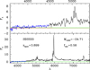 |
Fig. 3 As in Fig. 2 but for AGN SDSS20. |
| In the text | |
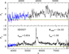 |
Fig. 4 As in Fig. 2 but for AGN SDSS27. |
| In the text | |
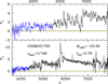 |
Fig. 5 As in Fig. 2 but for AGN COSMOS1782. |
| In the text | |
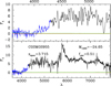 |
Fig. 6 As in Fig. 2 but for AGN COSMOS955. |
| In the text | |
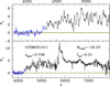 |
Fig. 7 As in Fig. 2 but for AGN COSMOS1311. |
| In the text | |
|
Fig. 8 UV spectrum of AGN COSMOS1710 observed by VLT FORS2. The spectroscopic redshift for this source in Marchesi et al. (2016) and Civano et al. (2016) turns out to be incorrect. The correct redshift is zspec = 1.547, thanks to many high-ionization lines detected in the spectrum (CIV, HeII, CIII, MgII, marked by the blue vertical lines). |
| In the text | |
|
Fig. 9 Bottom: UV/optical spectrum of the AGN SDSS36 observed by MODS1-2 at LBT. Top: a zoom of the blue side of the spectrum for AGN SDSS36. The red horizontal lines mark the zero level for the flux Fλ, in arbitrary units. The LyC region (at λ ≤ 912 Å rest frame) has been highlighted in blue. The associated RMS is shown by the green spectrum. The scientific data have been smoothed by a boxcar filter of 5 pixels. |
| In the text | |
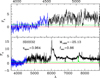 |
Fig. 10 As in Fig. 9 but for AGN SDSS32. |
| In the text | |
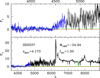 |
Fig. 11 As in Fig. 9 but for AGN SDSS37. |
| In the text | |
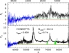 |
Fig. 12 As in Fig. 9 but for AGN COSMOS775. |
| In the text | |
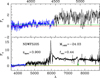 |
Fig. 13 As in Fig. 9 but for AGN NDWFSJ05. |
| In the text | |
|
Fig. 14 Bottom: the whole spectrum of the AGN SDSS3777 observed by LDSS3 at Magellan. Top: a zoom of the blue side of the spectrum for AGN SDSS3777. The red horizontal lines mark the zero level for the flux Fλ, in arbitrary units. The LyC region (at λ ≤ 912 Å rest frame) has been highlighted in blue. The associated RMS is shown by the green spectrum. The scientific data have been smoothed by a boxcar filter of 5 pixels. |
| In the text | |
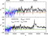 |
Fig. 15 As in Fig. 14 but for AGN SDSS3793. |
| In the text | |
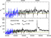 |
Fig. 16 As in Fig. 14 but for AGN SDSS3785. |
| In the text | |
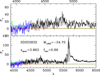 |
Fig. 17 As in Fig. 14 but for AGN SDSS3832. |
| In the text | |
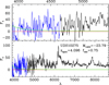 |
Fig. 18 As in Fig. 14 but for AGN UDS10275. |
| In the text | |
|
Fig. 19 Estimate of the LyC escape fraction for the AGN SDSS36 observed with MODS1-2 at the LBT telescope. The spectrum is in Fν and is arbitrarily normalized and blueshifted to z = 0 (rest-frame frequencies). The green portion of the spectrum shows the spectral region between 915 and 945 Å rest frame (excluding the wavelength range 935-940 Å due to the presence of the Lyman-ϵ emission line), while the magenta portion indicates the ionizing photons emitted between 892 and 905 Å rest frame. The blue vertical line indicates the location of the 912 Å rest-frame break. The red horizontal lines mark the mean values above and below the Lyman limit, after the iterative 2-σ clipping. The resulting escape fraction is the ratio between these two mean fluxes, and turns out to be 81% for SDSS36. |
| In the text | |
|
Fig. 20 Dependence of the LyC escape fraction on the absolute magnitude M1450 for QSOs and AGNs at 3.6 ≤ z ≤ 4.2. Squares show the targets observed with the VLT telescope, triangles are the AGNs observed with MODS1–2 at the LBT telescope, while pentagons are the AGNs observed with the LDSS3 instrument at the Magellan-II Clay telescope. The uncertainties on the measured LyC escape fraction at M1450 ≳−25 are of a few percent (~2–15%). The two asterisks connected by an horizontal line show the range of M1450 for the QSOs studied by Cristiani et al. (2016), while the three stars are three very bright QSOs (M1450 ~ −30) studied by Sargent et al. (1989, S89). No obvious trend of fesc with the absolute magnitude M1450 is detected. |
| In the text | |
|
Fig. 21 Dependence of LyC escape fraction on the observed U–I color for our faint AGNs. No obvious trend has been detected. Three objects from Table 1 have no information on the U-band magnitude and are not plotted here. |
| In the text | |
|
Fig. 22 HI photo-ionization rate measured by different estimators from the literature as a function of redshift. The magenta square shows the estimated value for the emissivity of AGNs at z ~ 4, assuming a luminosity function of Giallongo et al. (2015) down to M1450 = −18. The gray square indicates the contribution of faint AGNs adopting a luminosity function of Glikman et al. (2011). The green and violet squares indicate the AGN emissivity assuming a luminosity function of Parsa et al. (2018) and Akiyama et al. (2018), respectively. A LyC escape fraction of 75% has been assumed. The UVB derived by FG08 has been shown with filled blue circles, while we represent with open blue circles the same data of FG08 rescaled with a different temperature-density relation, as described in Calverley et al. (2011). |
| In the text | |
Current usage metrics show cumulative count of Article Views (full-text article views including HTML views, PDF and ePub downloads, according to the available data) and Abstracts Views on Vision4Press platform.
Data correspond to usage on the plateform after 2015. The current usage metrics is available 48-96 hours after online publication and is updated daily on week days.
Initial download of the metrics may take a while.