| Issue |
A&A
Volume 613, May 2018
|
|
|---|---|---|
| Article Number | A75 | |
| Number of page(s) | 24 | |
| Section | Stellar structure and evolution | |
| DOI | https://doi.org/10.1051/0004-6361/201731300 | |
| Published online | 05 June 2018 | |
Two-dimensional modeling of density and thermal structure of dense circumstellar outflowing disks
1
Department of Theoretical Physics and Astrophysics, Masaryk University,
Kotlářská 2,
611 37
Brno, Czech Republic
e-mail: This email address is being protected from spambots. You need JavaScript enabled to view it.
2
Institut für Physik und Astronomie, Universität Potsdam,
Karl-Liebknecht-Straße 24/25,
14476
Potsdam-Golm, Germany
Received:
2
June
2017
Accepted:
21
November
2017
Abstract
Context. Evolution of massive stars is affected by a significant loss of mass either via (nearly) spherically symmetric stellar winds or by aspherical mass-loss mechanisms, namely the outflowing equatorial disks. However, the scenario that leads to the formation of a disk or rings of gas and dust around massive stars is still under debate. It is also unclear how various forming physical mechanisms of the circumstellar environment affect its shape and density, as well as its kinematic and thermal structure.
Aims. We study the hydrodynamic and thermal structure of optically thick, dense parts of outflowing circumstellar disks that may be formed around various types of critically rotating massive stars, for example, Be stars, B[e] supergiant (sgB[e]) stars or Pop III stars. We calculate self-consistent time-dependent models of temperature and density structure in the disk’s inner dense region that is strongly affected by irradiation from a rotationally oblate central star and by viscous heating.
Methods. Using the method of short characteristics, we specify the optical depth of the disk along the line-of-sight from stellar poles. Within the optically thick dense region with an optical depth of τ > 2∕3 we calculate the vertical disk thermal structure using the diffusion approximation while for the optically thin outer layers we assume a local thermodynamic equilibrium with the impinging stellar irradiation. For time-dependent hydrodynamic modeling, we use two of our own types of hydrodynamic codes: two-dimensional operator-split numerical code based on an explicit Eulerian finite volume scheme on a staggered grid, and unsplit code based on the Roe’s method, both including full second-order Navier-Stokes shear viscosity.
Results. Our models show the geometric distribution and contribution of viscous heating that begins to dominate in the central part of the disk for mass-loss rates higher than Ṁ ≳ 10−10 M⊙ yr−1. In the models of dense viscous disks with Ṁ > 10−8 M⊙ yr−1, the viscosity increases the central temperature up to several tens of thousands of Kelvins, however the temperature rapidly drops with radius and with distance from the disk midplane. The high mass-loss rates and high viscosity lead to instabilities with significant waves or bumps in density and temperature in the very inner disk region.
Conclusions. The two-dimensional radial-vertical models of dense outflowing disks including the full Navier-Stokes viscosity terms show very high temperatures that are however limited to only the central disk cores inside the optically thick area, while near the edge of the optically thick region the temperature may be low enough for the existence of neutral hydrogen, for example.
Key words: stars: massive / stars: mass-loss / stars: winds, outflows / stars: evolution / stars: rotation / hydrodynamics
© ESO 2018
1 Introduction
Various types of stars are associated with equatorial disks. Notably, some of these disks can be classified as dense equatorial Keplerian outflowing disks which are typical for the classical Be stars or Pop III stars (Lee et al. 1991; Krtička et al. 2011; Kurfürst et al. 2014). The disk-like equatorial flows may also be formed around various classes of B[e] type stars (e.g., Hillier 2006), luminous blue variables (LBVs; e.g., Schulte-Ladbeck et al. 1994; Davies et al. 2005), post-asymptotic giant branch (post-AGB) stars (e.g., Heger & Langer 1998) or around the accretion inflows of, for example, young HAeB[e] stars (e.g., Thé et al. 1994). The possible formation channels of these disks include near-critical rotation, the wind confinement due to the magnetic field, or the effect of binarity.
In Keplerian outflowing disks, we assume that it is viscosity that plays a key role in the outward transport of mass and angular momentum (Lee et al. 1991) and governs the process of the disk creation and its further feeding and evolution. The disks are supposed to be rotationally supported and very thin in the region close to the star. Assuming a vertically isothermal gas, the disks are in vertical hydrostatic equilibrium with the Gaussian profiles of the density and pressure (e.g., Okazaki 1991). The vertical disk thickness (and also the disk vertical opening angle) grows with radius leading to the “flaring” shape of the disk. Also, observational evidence supports the idea that these gaseous disks are Keplerian, at least in the inner region, that is, approximately below the disk sonic point (Carciofi & Bjorkman 2008). Classical Be stars are on average the fastest rotators among all other (nondegenerate) types of stars. Their equatorial rotation rate is close to the critical limit (Rivinius et al. 2013). Whether the rotation of Be stars is (at least for a significant fraction of them) exactly critical, or mostly remains more or less subcritical, is still an open question that is intensively discussed. The determination of the observable projected rotational velocity vsin i is, in the case of rapid rotators, strongly affected by the stellar gravity darkening which makes the fast rotating equatorial area hardly observable (see, e.g., Townsend et al. 2004).
The existence of outflowing disks stems from the same principle as in the case of accretion disks, that is, the need for angular momentum transport. Evolutionary models of fast-rotating stars show that the stellar rotational velocity may approach the critical velocity (Meynet et al. 2006; Ekström et al. 2008), above which no stellar spin up is possible. The further evolution of critically rotating stars may require loss of angular momentum, which is carried out by an outflowing decretion disk (Krtička et al. 2011). The disk may in principle extend up to several hundreds of stellar radii (Kurfürst et al. 2014) or even more. The disk angular momentum transport requires some kind of anomalous viscosity, which we regard as being presumably connected with magnetorotational instability (Krtička et al. 2015).
The disk behavior, namely the distribution of density and the direction of the radial flow, may be far more complicated in models withvery high values of density or viscosity, or in the case of, for example, a central star with subcritical rotation (see Kurfürst et al. 2017). In such models, the occurrence of drops in radial velocity in the inner disk region indicates the material infall that may periodically increase the angular momentum of the inner disk, creating more or less regular waves of the density.
Apart from Be and Pop III stars, there may be another type of rapidly rotating star surrounded by a dense gaseous outflowing circumstellar disk: B[e] supergiants (sgB[e]s) (for a review see, e.g., Zickgraf 1998). These stars have a disk or a system of rings of high-density material containing gas and dust (Kraus et al. 2013). The origin of the B[e] phenomenon in evolved massive stars like sgB[e]s is still an open question. However, at least two possible fast rotating sgB[e] stars with rotation velocity reaching a substantial proportion (at least 70%) of critical velocity have been identified: the Small Magellanic Cloud stars LHA 115-S 23 (Kraus et al. 2008) and LHA 115-S 65 (Zickgraf 2000; Kraus et al. 2010). Another example is the Galactic eccentric binary system GG Car with a circumbinary ring, where two scenarios of ring origin have been discussed: either the nonconservative Roche lobe overflow or the possibility that, duringthe previous evolution of the system, the primary component underwent the classical Be star phase (Kraus et al. 2013). A particular subgroup of B[e] stars can also be identified with rapid rotators on a blue loop in Hertzprung-Russell (H-R) diagram (see Heger & Langer 1998, for details). Their disks could be formed by the spin-up mechanism induced by stellar contraction during the transition phase from red supergiant to the blue region on H-R diagram.
Most observable characteristics of the disks originate from regions at a distance up to ten stellar radii from the central star (Carciofi 2011). Therefore, the regions close to the star are key for understanding the observational behavior of stars with outflowing disks. As a first step towards more realistic multidimensional models, we provide detailed two-dimensional (2D) hydrodynamical simulations of central parts of the disk that include the radiative irradiation and viscous heating.
2 Basic equations of outflowing disk radial-vertical structure
Using our 2D models, we study the profiles of basic hydrodynamic and thermal characteristics in the radial-vertical plane in the inner dense Keplerian regions of the disks up to distance, which roughly corresponds to the sonic point radius of outflowing disks (Kurfürst et al. 2014). We examine the distribution of main characteristics of disks for various values of mass-loss rate, Ṁ = const. (Kurfürst et al. 2014), which is determined by the angular-momentum-loss rate needed to keep the star at or near critical rotation (Kurfürst 2012; Kurfürst & Krtička 2012, see also Krtička et al. 2011; Kurfürst et al. 2014). The basic scenario follows the model of the viscous decretion disk proposed by Lee et al. (1991, see also Okazaki 2001). The main uncertainty is the viscous coupling, namely the value and the spatial dependence of viscosity parameter α (Shakura & Sunyaev 1973). Despite some recent models indicating a constant viscosity throughout the disk (Penna et al. 2013), we have investigated the cases with variable α decreasing outward as a power law and examined various values of the disk base viscosity parameter α0.
The disk temperature is principally determined by the irradiation from the central star (Lee et al. 1991; Carciofi & Bjorkman 2008). The impinging stellar irradiation in the regions close to the star strongly depends on the geometry and other properties (equatorial and limb darkening) of the rotationally oblate central star. The stellar irradiation however does not deeply penetrate the central optically thick core of the disk (cf. Lee et al. 1991). If the disk mass-loss rate is relatively high, then the heating produced by viscous effects begins to dominate near the disk midplane. We study the distribution of temperature and the hydrodynamic structure of the dense disks corresponding to a final stationary state of self-consistent evolution of our 2D models, taking into account all the above-mentioned effects.
2.1 Hydrodynamic equations with vertical hydrostatic equilibrium
We study the self-consistently calculated radial-vertical structure of dense viscous outflowing disks assuming vertical hydrostatic equilibrium, that is, the vertical component of the disk gas velocity V z = 0. The basic hydrodynamic equations and the parameterization of one-dimensional (1D), radial, thin viscous disk structures are fully described in Kurfürst et al. (2014); see also, for example, Okazaki (2001) and Krtička et al. (2011). The cylindrical mass conservation (continuity) equation in the 2D axisymmetric (∂∕∂ϕ = 0, where ϕ is the azimuthal angle) case is
 (1)
(1)
where ρ is the density and V R(R, z) is the velocity of a radial outflow of the disk matter.
The corresponding radial momentum conservation equation is
 (2)
(2)
where V ϕ(R, z) is the disk azimuthal velocity, a(R, z) is the speed of sound, G is the gravitational constant, M⋆ is mass of the central star, and z is the vertical coordinate. The second and third terms on the right-hand side express the radial pressure gradient and radial component of gravitational acceleration, respectively. The explicit 2D form of the conservation equation of the angular momentum (cf. 1D Eq. (4) in Kurfürst et al. 2014 and Eq. (7.3) in Kurfürst 2015) is
 (3)
(3)
where the form of the full second-order Navier-Stokes viscosity term  (cf. 1D Eq. (9) in Kurfürst et al. 2014) is
![Mathematical equation: \begin{align*}f_{\text{visc}}^{(2)}=-\frac{1}{R}\frac{\partial}{\partial R}\left[\alpha a^2R^2\rho\left(1-\frac{\partial\ln V_{\phi}}{\partial\ln R}\right)\right]. \end{align*}](/articles/aa/full_html/2018/05/aa31300-17/aa31300-17-eq5.png) (4)
(4)
The term in the inner bracket is equal to 3∕2 in the case of Keplerian azimuthal velocity, V ϕ ~ R−1∕2, and it is equal to 2 in the case of angular momentum conserving azimuthal velocity, V ϕ ~ R−1. The contribution of the second-order viscous term is thus of significant importance and cannot be omitted, as most authors do. It also prevents the outer regions of the disk from switching to a physically implausible (negative) backward rotational motion (see Kurfürst et al. 2014).
We assume radial variations of viscosity parameter α introduced in Kurfürst et al. (2014),
 (5)
(5)
where α0 is the disk base viscosity, R is the cylindrical radial distance, Req is the stellar equatorial radius and n is a free parameter describing the radial viscosity dependence, n > 0. We employ in our models the values of the disk base viscosity parameter α0 = 0.025 (cf. Penna et al. 2013), α0 = 0.1, and α0 = 1. We regard the vertical profile of the viscosity as constant.
We do not employ the energy conservation equation in our calculations (neither do other authors who calculate the global structure of outflowing disks (Okazaki 2001, 2007; Sigut & Jones 2007)). Since the speed of sound plays a key role in gas dynamics, the flow characteristics are basically determined by subsonic or supersonic nature of the flow (see, e.g., Zel’dovich & Raizer 1967). In astrophysics, the temperature of the gas is very often determined by thermal balance between heat sources and radiative cooling. Radiative heating and cooling timescales are in this case quite short compared to other timescales in the problem, namely timescale of sound wave propagation (e.g., Shu 1992). It is therefore adequate to use the thermal balance in the present situation (Appendix 2.3), where the gas temperature is mainly determined by external processes (by irradiation of external sources, etc.).
 |
Fig. 1 Schema of the geometry of the disk irradiation by a central star. The disk “surface” element d S (with centralpoint B) is impinged by the stellar radiation coming along the line-of-sight vector d from the stellar surface element dS⋆ (with centralpoint A). Here α is the angle between the position vector of the point A and the vector d, β′ is the angle between normal vector ν of the surface element dS and the line-of-sight vector d, β = π∕2 − β′, and γ is the angle between normals of the surface element dS and of the equatorial plane. The idea is adapted from Smak (1989). |
2.2 The disk irradiation by the central star
The total radiative (frequency integrated) flux  from the whole “visible” stellar surface, intercepted by the surface element d S of the disk (see the notation in Fig. 1) is (Mihalas 1978)
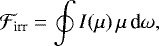 (6)
(6)
where I is the intensity of stellar radiation, μ = cosα, and d ω is the solid angle “filled” with the element dS as it is “seen” from the center of the stellar surface element dS⋆ (from the point A). From equalities I μ dω = Icosβ′ dω′ = Isinβ dω′, where d ω′ is the solid angle “filled” with the stellar surface element dS⋆ as it is “seen” from the point B, we obtain dω′ = dS⋆ μ∕d2, where d is the magnitude of the line-of-sight vector d.
We calculate the stellar equatorial (gravity) darkening by expressing the radiative flux F⋆ from rotationally oblate stellar surface in dependence on the stellar angular velocity Ω and stellar colatitude ϑ as (von Zeipel theorem, von Zeipel 1924; Maeder 2009, page 72)
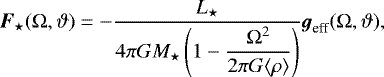 (7)
(7)
where L⋆ is the total stellar luminosity, ⟨ρ⟩ is the mean density of the stellar body, and geff is the vectorof effective gravity that is normal to the stellar surface,
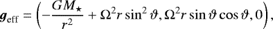 (8)
(8)
for stellar coordinate directions r, ϑ, φ, respectively (we hereafter distinguish between the spherical radial coordinate r and cylindrical radial coordinate R). In the case of critical rotation, the term in parentheses in the denominator of Eq. (7) is approximately 0.639 (see the Table 4.2 in Maeder 2009). The von Zeipel theorem in the case of a differentially rotating star differs only very slightly from Eq. (7) (Maeder 1999). We approximate the total stellar luminosity L⋆ as the luminosity for selected effective temperature of the oblate star with average stellar radius ⟨r⟩ given at the colatitude sin 2 ϑ = 2∕3 which corresponds to the radius at the root  of the second Legendre polynomial (cf. Maeder 2009, page 80). For example, in the case of critical rotation, ⟨r⟩ ≈ 1.1503 R⋆ (where R⋆ is the stellar polar radius).
For calculation of the limb darkening of the central star, we involve only the basic linear limb-darkening law. The specific intensity I of stellar irradiation is in this case modified as (see, e.g., Wade & Rucinski 1985; Heyrovský 2007)
![Mathematical equation: \begin{align*}I(\mu)=I(1)[1-u(1-\mu)], \end{align*}](/articles/aa/full_html/2018/05/aa31300-17/aa31300-17-eq12.png) (9)
(9)
with I being the intensity of the radiation for a given point on the stellar surface and u is the coefficient of the limb darkening that determines the shape of the limb-darkening profile. Integrating Eq. (9) over, for example, the “upper” hemisphere of the star (cf., e.g., Mihalas 1978; Smak 1989), we obtain the radiative flux from one half of the stellar surface (impinging “one side” of the disk), corresponding to a given point on the stellar surface as
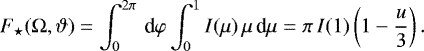 (10)
(10)
We adopt in our calculations the values of the linear limb-darkening coefficient u from Table 1 in van Hamme (1993).
The area of the stellar surface element dS⋆ of the rotationally oblate star (see Fig. 2) in spherical coordinates is
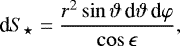 (11)
(11)
where cosϵ is cosine of the angle between the position vector r of a point on stellar surface and the vector geff of effective gravity (cf. Maeder 2009, page 27),
![Mathematical equation: \begin{align*}\cos\epsilon=\left[\left(\frac{R_{\star}}{r}\right)^2-\frac{8}{27}\left(\frac{\mathrm{\Omega}}{\mathrm{\Omega}_{\text{crit}}}\right)^2\frac{r}{R_{\star}}\sin^2\vartheta\right] \frac{g_{\text{pole}}}{g_{\text{eff}}}, \end{align*}](/articles/aa/full_html/2018/05/aa31300-17/aa31300-17-eq15.png) (12)
(12)
where Ωcrit is the angular velocity of the critically rotating star,  is the magnitude of the vector ggrav at the stellar pole, and geff is the magnitude of the vector geff.
The magnitude d of the line-of-sight vector d, where we note that the position vectors of the points A and B (see Fig. 1) are rA = r, rB = (R, 0, z), is
 (13)
(13)
From Eq. (8) the cosine of the angle between vectors g eff and d is (cf. Smak 1989; McGill et al. 2011)
![Mathematical equation: \begin{align*}\mu=\cos\alpha=\frac{A\left(R\cos\varphi-r\sin\vartheta\right)\sin\vartheta+B\cos\vartheta}{\left[A^2\sin^2\vartheta+C^2\right]^{1/2}d}\geq 0, \end{align*}](/articles/aa/full_html/2018/05/aa31300-17/aa31300-17-eq18.png) (14)
(14)
where A = 1∕r2 −Ω2r∕GM⋆, B = z∕r2 − cosϑ∕r and C = cosϑ∕r2. The inequality cosα ≥ 0 eliminates the line-of-sight vectors that connect the selected disk points with the “invisible” points on the stellar surface.
Following the simplified linear interpolation approximation corresponding to the “flaring disk” (see Figs. 1 and A.1), tanγ = (z∕H)ΔH∕ΔR, where H = H(R) is the disk vertical scale height (see Eq. (35)) and where ΔH and ΔR are the differences of these quantities within the radially neighboring computational cells (see the details of numerical grid described in Sect. 3). From this we obtain the normal vector ν to each disk surface element dS in the arbitrary disk point B(R, 0, z)
![Mathematical equation: \begin{align*}\boldsymbol{\nu}=\left[-z\left(\frac{{\mathrm{\Delta}} a}{a}+\frac{3}{2}\frac{{\mathrm{\Delta}} R}{R}\right),0,{\mathrm{\Delta}} R\right], \end{align*}](/articles/aa/full_html/2018/05/aa31300-17/aa31300-17-eq19.png) (15)
(15)
where a is the speed of sound and Δa is its difference between the radially neighboring computational cells.
Calculation of the angle β between this interpolated “disk surface” plane at arbitrary point B and the line-of-sight vector d gives the following relation,
![Mathematical equation: \begin{align*}\sin\beta=\frac{z\left[\left(a+\right)\left(R+\right)^{3/2}-1\right]\left(R-\right)+ {\mathrm{\Delta}} R\left(z-\right)} {\left\{z^2\left[\left(a+\right)\left(R+\right)^{3/2}-1\right]^2+({\mathrm{\Delta}} R)^2\right\}^{1/2}d}\geq 0, \end{align*}](/articles/aa/full_html/2018/05/aa31300-17/aa31300-17-eq20.png) (16)
(16)
where  ,
,  ,
,  and
and  . In the isothermal case the term
  is obviously equal to 1. The inequality sinβ ≥ 0 eliminates the line-of-sight vectors that come from below the local “disk surface” plane. This condition is further enforced by the stellar surface “visible domain” condition,
  , where r is the spherical radial coordinate of the point on stellar surface with height z(Req). This condition eliminates the stellar irradiation that comes to point B(R, z) from the star’s equatorial belt that lies below the vertical level z(Req)∕H(Req) ≤ z∕H(R). Following Eqs. (6)–(16) together with the described conditions, we integrate the (frequency integrated) stellar irradiative flux impinging each point B in the disk over the whole “visible” domain of the stellar surface. We obtain the following relation (cf. Eq. (6)),
![Mathematical equation: \begin{align*}\mathcal{F}_{\text{irr}}=\frac{1}{\pi}\!\!\iint_{\vartheta,\varphi}\!\! F_{\star}(\mathrm{\Omega},\vartheta)\,\text{d} S_{\star} \frac{\left[1-u(1-\mu)\right]\,\mu\sin\beta}{\left(1-u/3\right)\,d^2}, \end{align*}](/articles/aa/full_html/2018/05/aa31300-17/aa31300-17-eq27.png) (17)
(17)
where the radiative flux F⋆(Ω, ϑ) that emerges from the stellar surface is given by Eq. (7).
 |
Fig. 2 Schema of the rotationally oblate star with polar radius R⋆, equatorial radius Req, and stellar surface element dS⋆ whose position vector is r (with magnitude r). The vector geff is normal to the stellar surface element dS⋆. The angle ϵ denotes the deviation between the vectors ggrav (which is antiparallel to vector r) and g eff. |
2.3 Vertical temperature structure
Following Pringle (1981) and Frank et al. (2002), we express the viscous heat (or thermal) flux Fvis(R) per unit area of the disk in the 1D approach (taking into account two sides of the disk) as
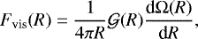 (18)
(18)
where  is the viscous torque exerted by the outer disk ring on the inner disk ring,
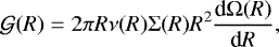 (19)
(19)
where Σ(R) is the vertically integrated (surface) density
 (20)
(20)
The kinematic viscosity ν = αaH (Shakura & Sunyaev 1973) can be, in the 2D case (neglecting vertical variations of angular velocity which is legitimate in the inner parts of the disk), expressed in the form
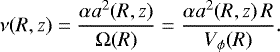 (21)
(21)
From Eq. (21), assuming hydrostatic and thermal equilibrium in the vertical direction (cf. Lee et al. 1991), which applies in the optically thick equatorial disk region that is not too far from the central star, we write the viscous heat flux in height z as (see Eqs. (3.18) and (3.28) in Kurfürst 2015)
![Mathematical equation: \begin{align*}F_{\text{vis}}(R,z)=\frac{1}{2}\frac{\alpha a^2(R,z)}{\mathrm{\Omega}(R)}\left[R\frac{\text{d} \mathrm{\Omega}(R)}{\text{d} R}\right]^2\int_0^z\rho(R,z^{\prime})\,\text{d} z^{\prime}. \end{align*}](/articles/aa/full_html/2018/05/aa31300-17/aa31300-17-eq33.png) (22)
(22)
Integration from −∞ to ∞ in Eq. (22) gives Fvis(R) in Eq. (18). From Eq. (22), it follows that there is zero net flux in the disk midplane, Fvis(R, 0) = 0, which results from symmetry.
Using the equation for pressure, P(R, z) = a2(R, z) ρ(R, z), and neglecting the vertical temperature gradient, we obtain the vertical slope of the viscous heat flux in the form
![Mathematical equation: \begin{align*}\frac{\text{d} F_{\text{vis}}(R,z)}{\text{d} z}=\frac{1}{2}\frac{\alpha P(R,z)}{\mathrm{\Omega}(R)}\left[R\frac{\text{d}\mathrm{\Omega}(R)}{\text{d} R}\right]^2. \end{align*}](/articles/aa/full_html/2018/05/aa31300-17/aa31300-17-eq34.png) (23)
(23)
From vertical hydrostatic equilibrium (involving Eq. (32)) the vertical pressure gradient simultaneously follows:
 (24)
(24)
where we explicitly include the possibility of vertical variations of disk angular velocity (see Sect. 3 for details).
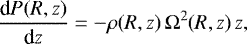
Assuming local thermodynamic and radiative equilibrium in the optically thick regions and omitting now the external radiative flux  (that we assume does not penetrate into optically thick layers), the vertical gradient of the temperature (e.g., Lee et al. 1991) generated by the viscous heating is
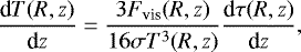 (25)
(25)
where σ is the Stefan-Boltzmann constant. The vertical gradient of the disk optical depth τ in Eq. (25) is
 (26)
(26)
where κ is the opacity of the gas in the disk (e.g., Mihalas 1978; Mihalas & Mihalas 1984). Equation (25) holds only in the case where the radiative gradient ∇rad does not exceed the adiabatic gradient, that is, ∇rad < ∇ad (see, e.g., Sect. 5.1.3 of Maeder 2009, for details). We therefore examined also the regions where convection may develop. However, because the adiabatic gradient for monoatomic perfect gas ∇ad = 2∕5, our calculations show that the convective zones occur only in the models with the highest densities, that is, with Ṁ ≥ 10−7 M⊙ yr−1 (see Sect. 4.2 and Lee et al. 1991).
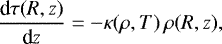
We include electron scattering, bound-free, and free-free opacities in our model. For the calculation of Thomson (electron) opacity of partly ionized hydrogen (where for fully ionized hydrogen κes ≈ 0.04 m2 kg−1 in SI units) we use the relation (Schwarzschild 1958; Mihalas 1978; Maeder 2009)
 (27)
(27)
where ne is the number density of free electrons, ρ is the gas density, σes is the Thomson scattering cross-section, σes ≈ 6.65 × 10⁻²⁹ m2, nN is the number density of all particles, that is, the sum of free electrons (which equals the number of hydrogen ions) and neutral hydrogen atoms, and mu is the atomic mass unit. The ratio ne∕nN is obtained from the Saha equation. We involve only hydrogen atoms for calculation of κes for simplicity.
We involve also the mean Roseland opacity for continuum, that is, κbf for bound-free and κff for free-free absorption according to assumed chemical composition of the disk material. In the case of only hydrogenic composition (like in pop III stars’ disks) we involve only the mean Roseland opacity for the free-free absorption. The bound-free and free-free opacities are roughly given by a Kramers law (cf. Eqs. (8.24) and (8.29) in Maeder 2009, cf. also, e.g., Schwarzschild 1958) in the form (also taking into account the rapid decrease of concentration of free electrons in the region with low temperatures, analogously to Eq. (27)),
 (28)
(28)
where X and Z are the mass fractions of hydrogen and metals, respectively, ρ is the gas density and T is temperature. The coefficients κ0,bf ≈ 4.3 × 10²¹ m5 kg−2 K7∕2 and κ0,ff ≈ 7.4 × 10¹⁸ m5 kg−2 K7∕2 (Maeder 2009). In the case of standard (solar) composition, bound-free opacity dominates over free-free opacity (e.g., in the case of solar composition with Z ≈ 0.02 the bound-free opacity by about an order of magnitude exceeds the free-free opacity), however, because the free-free opacity does not depend on metallicity, it dominates in very low-Z objects (e.g., in Pop III stars). Finally, the overall optical depth κ in Eq. (26) is the sum κ = κes + κbf + κff. For other details see the description of numerical approach in Sect. 3 and in Appendix A.5.
For inclusion of the effect of stellar irradiation we calculate the limit where the disk optical depth τ = 2∕3 (we denote it τ2∕3), regarding the line-of-sight from stellar pole (see more details in Sect. 3) and calculating self-consistently the hydrodynamic and thermal properties of the gas. We calculate the temperature T2∕3 at the optical depth limit τ2∕3 simply via the frequency integrated Eddington approximation (Mihalas 1978),
 (29)
(29)
where  is given by Eq. (17) and Fvis is determined by Eqs. (22) and (23). The temperature is then calculated as follows: the temperature T2∕3 is used as the starting point for calculation of the disk thermal and density structure in the optically thick domain with τ ≥ τ2∕3, using the diffusion approximation (excluding in the optically thick domain the effects of
  ) from thermal and hydrostatic equilibrium Eqs. (24)–(26). The computation is performed provided that the disk equatorial plane boundary condition Fvis(z = 0) = 0 is satisfied. In the optically thin domain (τ < τ2∕3) we calculatethe temperature from a local thermodynamic and radiative (gray) equilibrium of the gas with the impinging external flux of the stellar irradiation (using Eq. (29) with τ < τ2∕3 and omitting therein the contributionof the viscous heating Fvis). This approximation is relevant in this case since the temperature structure of the disk material is maintained primarily by an external source of energy, we therefore regard the hydrodynamic equation of state as isothermal (in principle, however, the solution of the optically thin environment is not the main point of these models).
We also involve the effect of radiative loss of energy, QT ≈ ρ2P(T), where P(T) is a positive function that describes the temperature variations of the radiative loss in the optically thin approximation, which however plays a significant role only above T ≈ 15 000 K (Rosner et al. 1978; Leenaarts et al. 2011; at lower temperatures the radiative energy is assumed to be mostly absorbed in continua of neutral helium and neutral hydrogen where it contributes to radiative heating and thus to internal energy of the outflowing gas (Carlsson & Leenaarts 2012)). For the calculation we adopt the values of function P(T) for various ranges of temperature in the optically thin domain from Eq. (A.1) in Rosner et al. (1978). The approximative boundary between the optically thick and optically thin domain is for the radiative loss calculated in the vertical direction z (unlike the heating, where the boundary of the optically thick region is calculated along the line-of-sight from the stellar pole). The decrease in temperature is then calculated similarly as in the case of the heating contribution, that is, with use of modified Eq. (29), where the last term in parentheses is replaced by the radiative cooling Fcool, determined by
 (30)
(30)
where nH is the number density of hydrogen particles (cf. Carlsson & Leenaarts 2012).
2.4 Initial state
The initial conditions are derived assuming Keplerian rotating disk. Integrating analytically the vertical hydrostatic equilibrium equation,
 (31)
(31)
where the vertical component of gravitational acceleration,
 (32)
(32)
and we can integrate the analytical expression for the initial density profile into the form
![Mathematical equation: \begin{align*}\rho=\rho_{\text{eq}}\,\text{exp}\left[-\frac{GM_{\star}}{a^2}\left(\frac{1}{R}-\frac{1}{r}\right)\right], \end{align*}](/articles/aa/full_html/2018/05/aa31300-17/aa31300-17-eq47.png) (33)
(33)
where ρeq = ρ(R, 0), which is the density in the equatorial plane (disk midplane where z = 0) and  . Equation (33) provides a more realistic 2D analytical profile of a disk spatial density than the usually used Gaussian vertical density distribution in a thin disk approximation. This becomes relevant for 2D models, which (due to a convergence necessity) extend up to several hundreds of stellar radii, where the assumption z ≪R does not hold.
To express the initial profile of the disk midplane density ρeq analytically, we employ the 1D equation of the vertically integrated density (e.g., Krtička et al. 2011),
 (34)
(34)
where we adopt the approximation Σ(R) ~ R−2 (e.g., Okazaki 2001). Denoting H the vertical disk scale height,
 (35)
(35)
where Ω is the angular velocity, we obtain for the Keplerian disk region  where ρ0 is the disk base density (noting that H ~ R3∕2 in the disk Keplerian region).
To determine the disk base density value ρ0, we first calculate the disk base surface density Σ 0 from a selected disk mass-loss rate Ṁ. We use the equation of mass conservation, Ṁ = 2πReqΣ0V R(Req), where we adopt the already pre-calculated density independent value of the disk base radial velocity V R (Req) from a 1D model (see Kurfürst et al. 2014; Kurfürst 2015, for details). We note that the value of the disk base integrated density Σ 0 (connected with the selected Ṁ) and the viscosity parameters α0 and n are the only parameters (except the parameters of central star) that stay fixed during the whole computational process. We finally obtain the initial disk volume base densityρ0 from Eq. (34) with use of Eq. (35), where we adopt an initial sound speed a in accordance with an initially parameterized temperature profile,
 (36)
(36)
where  is the disk base temperature (cf. Carciofi & Bjorkman 2008) and p is a slope parameter (where in the isothermal case p = 0).
Combining Eqs. (33)–(35), we write the initial density profile in the explicit form
![Mathematical equation: \begin{align*}\rho(R,z)= {\mathrm{\Sigma}}_0\left(\frac{R_{\text{eq}}}{R}\right)^2\sqrt{\frac{GM_{\star}}{2\pi a^2R^3}}\exp\left[\frac{GM_{\star}}{a^2R}\left(\frac{R}{r}-1\right)\right]. \end{align*}](/articles/aa/full_html/2018/05/aa31300-17/aa31300-17-eq54.png) (37)
(37)
The initial profile of the outflowing disk angular momentum J takes, in 2D models, the explicit form
 (38)
(38)
where the radial component gR(R, z) of the external gravity is given by the radial analog of Eq. (32). The initial radial and vertical components of momentum are
 (39)
(39)
in the whole computational domain. We describe boundary conditions in Sect. 3 while some additional or specific initial and boundary conditions may be also described in sections that refer to specific models.
3 Numerical methods
For the disk modeling we have developed and used two types of hydrodynamic codes based on different principles: (1) the operator-split (ZEUS-like) finite volume Eulerian numeric schema on staggered mesh for the 2D (relatively) smooth hydrodynamic calculations (Stone & Norman 1992) and (2) our own version of a single-step (unsplit, ATHENA-like) finite volume Eulerian hydrodynamic algorithm based on the Roe’s method (Roe 1981; Toro 1999). We originally developed the latter code for a different astrophysical problem with highly discontinuous flows, however, we employed the code also to test our calculations of the 2D disk structure (see the description in Appendices A.6–A.8). We have calculated our models several times with various parameters using both the code types, obtaining practically identical results.
For the time-dependent calculations, we write the left-hand sides of hydrodynamic Eqs. (1)–(3) in conservative form (see, e.g., Norman & Winkler 1986; Hirsch 1989; Stone & Norman 1992; Feldmeier 1995; LeVeque et al. 1998)
 (40)
(40)
where u = ρ, ρV, R× ρV and F(u) = ρV, ρV | V, R× ρV | V for the mass, momentum, and angular momentum conservation equations, respectively, where × denotes the vector product and| denotes the dyadic product of two vectors of velocity.
The source steps, that is, the right-hand sides of Eqs. (2) and (3), express the action of external forces (gravity) and internal pressure forces on the gas (see Norman & Winkler 1986) in the standard cylindrical coordinates. We solve finite-difference approximations of the following differential equations in the approximative Lagrangian form (Stone & Norman 1992),
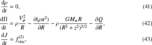
where Π = ρV R is the radial momentum density, J is the angular momentum density, and  is the second-order viscosity term derived in Eq. (4).
We use the following boundary conditions for particular hydrodynamic quantities at the inner boundary (at stellar surface): here the density ρ and the angular momentum J are fixed (assuming constant mass flow and the permanent Keplerian azimuthal velocity) while the radial momentum flow Π R and the vertical momentum flow Πz are free, that is, the quantities are extrapolated there from the neighboring grid interior values as a 0th-order extrapolation. We set the free (outflowing) outer boundary conditions for all the quantities. We assume the lower and upper (vertical) boundary conditions as outflowing (or alternatively periodic, which does not significantly affect the calculation), see also Kurfürst et al. (2014) and Kurfürst (2015).
In order to smooth out the discontinuities which occur when shocks are present, the operator-split staggered mesh type of numeric schema involves the artificial viscosity (von Neumann & Richtmyer 1950) which is in general described by a tensor (Schulz 1964). We employ (in the ZEUS-like code) merely the scalar artificial viscosity Q (providing the same practical results as the tensor) in the explicit form (Norman & Winkler 1986; Caramana et al. 1998),
![Mathematical equation: \begin{align*}Q_{i,k}=\rho_{i,k}\,{\mathrm{\Delta}} V_{R,i,k}\,[-\text{C}_1a_{i,k}+\text{C}_2\text{min}({\mathrm{\Delta}} V_{R,i,k},0)], \end{align*}](/articles/aa/full_html/2018/05/aa31300-17/aa31300-17-eq60.png) (44)
(44)
where ΔV R,i,k = V R,i+1,k − V R,i,k is the forward difference of the radial velocity component, a is the sound speed and the lower indices i, k denote the ith and kth radial and vertical spatial grid cells. The second term scaled by a constant C 2 = 1.0 is the quadratic artificial viscosity (see Caramana et al. 1998) used in compressive zones. We use the linear viscosity term for damping oscillations in stagnant regions of the flow (Norman & Winkler 1986). We use this term with the coefficient C 1 = 0.5 only rarely, whensome numeric oscillations occur, for example, in the inner disk region near the stellar surface.
We use spherical coordinates in order to define the maximally uniform mesh covering the rotationally oblate stellar surface. The spherical coordinate ϑ (stellar colatitude – not to be confused with the θ coordinate in the flaring coordinate system, see Appendix A) ranges approximately from 0 to π∕2 assuming that the irradiation comes to the “upper” disk “surface” only from the “upper” stellar hemisphere. Following the Roche model (for a rigidly rotating star with most of its mass concentrated to stellar center) we obtain the spherical radial distance r of each grid point on the stellar surface for each given colatitude ϑ by finding the root of the equation (e.g., Maeder 2009, p. 24)
 (45)
(45)
where Ω is the angular velocity of the stellar rotation, R⋆ is the stellar polar radius and Ωcrit is the angular velocity of the star in case of critical rotation. The stellar azimuthal φ direction ranges from − π to π in order to take into account also the stellar irradiation that emerges from the stellar surface behind the meridional circle impinging the disk regions with high vertical coordinate z. Both stellar ϑ and φ domains aredivided into 100 grid-cell intervals.
From the computational point of view, the fundamental problem of the 2D self-consistent disk modeling in the R-z plane is the disproportional increase of the disk vertical scale height H within a distance of a few stellar radii (from Eq. (35) follows H ∝ R3∕2 in the inner Keplerian region and H ∝ R2 in the outer angular momentum conserving region). To avoid this difficulty, we have developed a specific type of non-orthogonal (we call it “flaring”) grid, which is a kind of hybrid of cylindrical and spherical spatial mesh. We convert Eqs. (41)–(39) into the “flaring” system using transformation equations introduced in Appendix A where we analyze the grid geometry in detail. The aim of introducing such a grid was to exclude the points with high z and low R (see Fig. A.1) from the calculation. The disk density is very low in these regions, therefore they are irrelevant for the disk dynamics. On the other hand, we have to involve the regions with high z at greater distance from the star (cf. Kurfürst 2015). We also describe the explicit form of the Roe matrices used in the single-step code version, re-calculated for the “flaring” coordinate system, in Appendices A.6 and A.7. The gas hydrodynamic computations on the flaring grid successfully run up to (at least) 1000 R⋆. On the other hand, we did not use the grid for magnetohydrodynamic calculations for its great mathematical complexity. Another possibility may be the usage of a kind of structured quadrilateral mesh, presented, for example, in Chung (2002) with static mesh refinement multigrid hierarchy. The viability of the flaring system for various purposes and conditions will be the subject of additional testing.
We have also made attempts to calculate some models with the vertical hydrostatic equilibrium included merely as an initial state, while in the further evolution, the hydrostatic equilibrium is numerically switched off. However, such calculations have not yet been successful due to a violent computational instability after a few time steps. The likely reason is too overly temporal and spatial variation of all quantities (unlike, e.g., in the isothermal and non-viscous model of Kee et al. 2016), including the crossing of the transforming wave (see Sect. 4.1). Further testing and fine-tuning of the numeric schema is need at this point. For this reason the current numerical calculations are performed by updating the vertical hydrostatic balance within each time step.
In the operator-split smooth hydrodynamic code, we calculate the time step Δ t employing the predefined Courant-Friedrichs-Lewy (CFL) number C0 ≤ 1∕2 (Stone & Norman 1992). The directionally split algorithm (where for simplicity we write the standard cylindrical z coordinate while the “flaring” form of the algorithm may be an analog of Eq. (A.70)) is
 (46)
(46)
where a is the isothermal speed of sound. We denote the contribution of the numerical viscosity to the time increment as Δ tvis where (Stone & Norman 1992)
 (47)
(47)
The factor 4 in the denominator of Eq. (47) results from the transformation of the momentum equation into the diffusion equation due to the inclusion of the artificial viscosity. The time step is calculated using the relation (Norman & Winkler 1986; Stone & Norman 1992)
![Mathematical equation: \begin{align*}{\mathrm{\Delta}} t=C_0\left[\left({\mathrm{\Delta}} t_R\right)^{-2}+ \left({\mathrm{\Delta}} t_z\right)^{-2}+\left({\mathrm{\Delta}} t_a\right)^{-2}+\left({\mathrm{\Delta}} t_{\text{vis}}\right)^{-2}\right]^{-1/2}; \end{align*}](/articles/aa/full_html/2018/05/aa31300-17/aa31300-17-eq64.png) (48)
(48)
the algorithm thus checks the Courant stability theorem by controlling the time step according to all the relevant physical conditions.
We calculate the interface between the optically thin and optically thick regions in the disk along the line-of-sight from stellar pole (see the basic description in Sect. 2.3 and details in Appendix A.5). We use the method of short characteristics for tracing the path of each ray that passes through the nodes of the grid (see Fig. A.2). For each node of the disk grid located in the optically thin domain we find the distance d (see Eq. (13)) from each “visible” node of the stellar surface grid. We calculate the impinging stellar irradiation  according to Eq. (17) as a numerical quadrature neglecting the absorption of the flux in the optically thin region. We assume the flux
  is fully thermalized in the optically thin region taking into account radiative cooling using the optically thin approximation (see Sect. 2.3). The temperature profile in the optically thick domain is calculated as the diffusion approximation using Eqs. (18)–(29) in Sect. 2.3.
We performed all the calculations, employing both the methods introduced in this Section, on a numerical grid logarithmically scaled in the radial direction, with the outer radius of the computational domain 500 Req. The purpose of using such a relatively large domain is to achieve a region with smooth profiles in the characteristics of the outer boundary, which are necessary for the proper convergence of the models. The results introduced in the following Sections are therefore merely the illustrative fragments of the total computational domain. The number of spatial grid cells is 500 in the radial and 200 in the vertical direction (where the R distance is logarithmically scaled). The computational time was approximately one week (the maximum number of parallel processes used was 100). The physical time of the convergence of the models is identical to dynamical times introduced in Sect. 4.1.
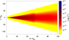 |
Fig. 3 Snapshot of the density wave propagating in the distance R ≈ 55Req in the converging 2D model of the isothermal outflowing disk (cf. the disk-forming density wave in 1D models in Kurfürst et al. 2014), calculated in the R-z (R-θ) plane. The elapsed time since the start of the simulation is approximately 80 days. The parameters of the critically rotating B0-type parent star are introduced in Table 1. The sonic point is beyond the displayed domain (Rs ≈ 5.5 × 10² Req). The model is calculated using the flaring grid whose prescription is given in Appendix A. The initial disk midplane density is determined by the stellar mass-loss rate Ṁ = 10−9 M⊙ yr−1 and the viscosity is parameterized as α = α0 = 0.025 (Penna et al. 2013). |
4 Results of numerical models
4.1 Disk evolution time
In the 2D hydrodynamic time-dependent models we recognize the same transforming wave as in our 1D models (described in detail in Kurfürst et al. 2014) that converges the disk initial state to its final stationary state. The wave occurs during the disk-developing phase in all types of disks (Sects. 4.2 and 4.3) and it may effectively determine the timescale of the circumstellar disk growth and dissipation periods (e.g., Guinan & Hayes 1984; Štefl et al. 2003). In the subsonic region the wave establishes nearly hydrostatic equilibrium in the radial direction (see Eq. (2)), while its speed approximately equals the speed of sound. According to our 1D models (Kurfürst et al. 2014) the wave propagates in the supersonic region as a shock wave that is slowed down, compared to the subsonic region, to approx. 0.5–0.3 a. However, we cannot yet verify this prediction in 2D self-consistent models since we have not yet been able to extend the calculations significantly above the sonic point distance due to the enormous computational cost.
In an isothermal disk (with p = 0 in Eq. (36)) the propagation time of the transforming wave in the subsonic region is the dynamical time (see the discussion in Sect. 5.2. of our foregoing paper Kurfürst et al. 2014)
 (49)
(49)
We note that the dynamical time is almost independent of the viscosity while it significantly increases with decreasing temperature. Figure 3 demonstrates the snapshot of the time evolution of the density in a 2D isothermal model calculated using the flaring grid (see Appendix A). The figure shows the transforming wave that is currently propagating roughly in the middle of the radial domain. The central star is in this case the B0-type star with the parameters given in Table 1, with the viscosity parameter α = α0 = 0.025 (Penna et al. 2013). The initial and boundary conditions are identical to those described in Sects. 2.1 and 3; we however employ the initial (Keplerian) azimuthal velocity profile defined as  , where gR (R, z) is the radial component of gravitational acceleration. The initial disk midplane density is determined by the mass-loss rate Ṁ = 10−9 M⊙ yr−1 (selected as a free parameter). For example for the two distances, 50 Req and 100 Req, the 2D model gives from Eq. (49) tdyn ≈ 0.6 yr and 1.2 yr, respectively.
To derive an estimate of the dynamical time in our nonisothermal models, we neglect the vertical variations of temperature and fit the disk midplane temperature by a power law Eq. (36). The dynamical time is from Eqs. (49) and (36)
 (50)
(50)
where  is the speed of sound at the base of the disk, k is the Boltzmann constant, μ is the mean molecular weight (for simplicity we hereafter use μ = 0.62 for the fully ionized hydrogen-helium plasma), and mu is the atomic mass unit. Using this relation we can compare the values of tdyn in the non-isothermal models. As an example, the analytical estimate of the dynamical time in the model introduced in Sect. 4.2 with Ṁ = 10−6 M⊙ yr−1, given by Eq. (50) (with T0 ≈ 80 000 K and p ≈ 0.7 derived from the fit of the numerical model), is tdyn ≈ 4.4 yr for the distance 50 R∕Req while the numerical model gives the value tdyn ≈ 3.9 yr.
Stellar parameters for B0-type star (Harmanec 1988, see also Kurfürst et al. 2014) and for typical Pop III star (e.g., Marigo et al. 2001) used in the models.
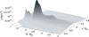 |
Fig. 4 2D graph of the density of the converged model of a circumstellar viscous outflowing disk of a (near) critically rotating star in the very inner region up to 5 stellar radii, corresponding to the disk mass-loss rate Ṁ = 10−6 M⊙ yr−1, with the constant viscosity parameter α = α0 = 0.1. The parameters of the star correspond to average parameters of Pop III stars (see Table 1) or sgB[e] stars (e.g., Kraus et al. 2007). The sonic point is in this case at a distance of approximately 2 × 10⁴ Req. The density profile shows in this case irregular bumps in the very inner disk region. The contours mark the density levels (from lower to higher) 10−9, 10−8, 10−7, 10−6, 2.5 × 10⁻⁶, 5 × 10⁻⁶ [kg m −3], and so on, with a constant increment of 2.5 × 10⁻⁶ kg m−3. |
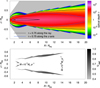 |
Fig. 5 Upper panel: color map of the profile of the optical depth in the inner part (up to 20 stellar equatorial radii) of the dense circumstellar outflowing disk of a (near) critically rotating star with the same parameters as in Fig. 4. The optical depth is calculated using the method described in Appendix A.5. The outer black contour traces the optical depth level τ = 0.75 that is calculated along the line-of-sight from the stellar pole (described as “along the ray” in the figure legend), while the blue contour traces the same optical depth calculated along the vertical (z axis) direction. The inner black contour traces the optical depth level τ = 2500 that is calculated along the line-of-sight from the stellar pole. Lower panel: map of the convective zones with ∇rad > ∇ad on the same scale. The large zones refer to the disk mass-loss rate Ṁ = 10−6 M⊙ yr−1 while the small wings near the disk base refer to Ṁ = 10−7 M⊙ yr−1. |
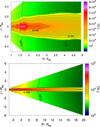 |
Fig. 6 Upperpanel: color map of the temperature distribution in the very inner part (up to 5 stellar equatorial radii) of the dense circumstellar outflowing disk of a (near) critically rotating star with the same parameters as in Fig. 4. The region of significantly increased temperature near the disk midplane is generated by the viscous heating. The contours mark the temperature levels 5000 K, 10 000 K, 20 000 K, 50 000 K and 80 000 K. Lower panel: as in the upper panel, in theinner part up to 20 stellar equatorial radii. The strip of highly increased temperature near the disk midplane is generated by the viscous heating. The contours mark the temperature levels 3000 K, 10 000 K and 50 000 K. |
4.2 Models of massive dense disks with disk mass-loss rate Ṁ > 10−8 M⊙ yr−1
We have examined a great variety of models with different parameters, from the highest disk mass-loss rate Ṁ = 10−5 M⊙ yr−1 that may correspond to the most massive outflowing disks of Pop III stars (Marigo et al. 2001; Ekström et al. 2008) or sgB[e]s (Kraus et al. 2007, 2010) to the lowest ones, Ṁ = 10−11 M⊙ yr−1, corresponding to classical Be star disks (e.g., Carciofi & Bjorkman 2008). The reason why we introduce disk models with the mass-loss rate higher or lower than approximately Ṁ ≈ 10−8 M⊙ yr−1 separately in different Sections is that the higher ones may correspond to massive disks of giant stars like sgB[e]s or Pop III stars, while the lower ones dominantly represent the disks of classical Be stars (although the transition may not be accurate nor sharp).
Our calculation showed that the results of the models with disk mass-loss rates Ṁ = 10−5 M⊙ yr−1 and Ṁ = 10−6 M⊙ yr−1 are qualitatively similar and differ only by the density and temperature. Figure 4 shows the distribution of the self-consistently calculated density in the very inner region of the disk (up to 5 Req) in the model with disk mass-loss rate Ṁ = 10−6 M⊙ yr−1 and the constantviscosity α = α0 = 0.1. The parameters of the central Pop III (or sgB[e]) star are introduced in Table 1 (we assume for simplicity zero metallicity in this type of disks).
Irregular bumps of the density occur in these high-density models that may be connected with the (more or less regular) drops in radial velocity V R to negative values, which indicate the material infall that periodically increases the angular momentum of the inner disk, creating the density waves (cf. the density waves in the model with lower density, but with the high-viscosity parameter, in the lower panel in Fig. 9, vs. the smooth density profile in the model with relatively low density and viscosity in the upper panel of Fig. 9). The time scale of this process is however quite fast; of the order of hours or days. For a better estimation, we need to simulate this particular disk behavior on much shorter time-scales, probably using the local computational schema focused on a small region of a disk.
We attach in Fig. 8 the graphs of radial velocity V R and azimuthal velocity V ϕ in the innerdisk region (up to 20 stellar radii) of the converged disk, calculated within the 2D model of the disk of the Pop III star with parameters given in Table 1 with Ṁ = 10−6 M⊙ yr−1. As we may expect kinematically, both the velocities show maximum vertical values in the disk midplane while with increasing |z| the velocities are lower. However, the calculations do not include the effects of ablation of the disk’s surface layers due to strong radiation (cf. Kee et al. 2016). Equation (1) (with use of Eq. (20)) implies that Ṁ = const. throughout the stationary disk (see also Kurfürst et al. 2014). We do not show the profile of the angular-momentum-loss rate  since it basically corresponds to the profiles introduced in Kurfürst et al. (2014), that is, the rate increases up to approximately the sonic point radius.
All the models with Ṁ > 10−9 M⊙ yr−1 (see Figs. 4 and 9 as well as the corresponding chart of the temperature in Fig. 6) show the permanent bump of the density (and of pressure and temperature) at the radius 1.5– 3.5 Req produced bylarge viscous friction together with the increase of the rate of external heating at the particular distance (due to stellar oblateness). This causes the rapid increase of disk vertical scale height (see Eq. (35), which becomes significant in the models with high disk density. This, in turn, leads to formation of the “inner torus” in the models (cf. the accretion disk morphology in Balbus 2003, however, the formation mechanism is in this case likely quite different).
We also examined the zones of possible influence of convection (see the lower panel in Fig. 5 which maps the convective zones with ∇rad > ∇ad; see also the description in Sect. 2.3), however we do not model the convective process itself. In agreement with Lee et al. (1991), we found the formation of convective zones only in the models with Ṁ ≥ 10−7 M⊙ yr−1. The largest disk convective zone (as expected) develops in the model with Ṁ ≥ 10−6 M⊙ yr−1; its inner boundary is at the radius R ≈ 2 Req, and it is developed in the relatively narrow strip near the line of optical depth level τ ≈ 1 (see Fig. 5) up to the radius R ≈ 14 Req. The convective zone is drastically reduced to the area between R ≈ 2–3 Req and |z|≈ 0.05–0.15 Req in the model with Ṁ = 10−7 M⊙ yr−1. The convective zones, which may also be connected with and enhanced by the effects of hydrogen ionization, contribute to the increase of the disk optical depth (cf. Lee et al. 1991). However, the permanent bump (although more subtle and more distant) occurs also in the models without the convection (see, e.g., Fig. 9).
The upper panel in Fig. 5 shows the distribution of the optical depth in the very massive disk model with Ṁ = 10−6 M⊙ yr−1. The highestoptical depths in the disk midplane in particular models in this section are τ ≈ 4000 at the radius R ≈ 1.5 Req in the model with Ṁ = 10−6 M⊙ yr−1, while this is reduced to τ ≈ 200 at the radius R ≈ 1.1 Req in the model with Ṁ = 10−7 M⊙ yr−1.
The resulting radial-vertical temperature structure of the dense disk models up to 5, 20 and 50 stellar radii is plotted in Figs. 6 and 7. The maximum temperatures are T ≈ 80 000 K and T ≈ 40 000 K in the disks with Ṁ = 10−6 M⊙ yr−1 and Ṁ = 10−7 M⊙ yr−1, respectively, and the regions with maximum temperature roughly correspond to the regions with highest optical depth. The disks with Ṁ ≥ 10−6 M⊙ yr−1 show (with particular stellar parameters) significant strip of increased temperature up to the radius R ≈ 50 Req. In this point we note that the sonic point radius for the disks with given parameters is approximatively at 2 × 10⁴ Req. We also tested the models with higher disk base viscosity, however, the resulting temperature profiles differ only by a few percents. The models with radially decreasing viscosity (where n > 0 from Eq. (5)) give the same results as the introduced models with constant viscosity, the differences in the models with decreasing viscosity are evident only at much larger distances from the central star (see our 1D models in Kurfürst et al. 2014).
The detection of strong [OI] line emission in sgB[e] disks (Kraus et al. 2007) implies a presence of high density region that is neutral in hydrogen (6000 K ≲ T ≲ 8000 K). Assuming a viscous disk, the temperatures near the disk core are too high due to the viscous heat generation. However, since the temperature contour 10 000 K is inside the optically thick region (τ ≳ 0.75), the neutral hydrogen emitting layer could possibly be located near the transition from an optically thin to thick region.
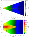 |
Fig. 7 Upper panel: as in Fig. 6, up to the intermediate distance of 50 stellar equatorial radii. The near-equatorial strip of enhanced temperature exceeds in this case the distance 50 Req. The contours mark the temperature levels 1000 K, 2000 K, 5000 K and 10 000 K. Lower panel: color map of the temperature distribution in the very inner part (up to 5 stellar equatorial radii) of the dense circumstellar outflowing disk of a (near) critically rotating star with the same parametersas in Fig. 4, however, the parameterized disk mass-loss rate is in this case Ṁ = 10−7 M⊙ yr−1. The region of increased temperature generated by the viscous heating near the disk midplaneis in this case significantly reduced and extends up to only approximatively 4 Req. The contours mark the temperature levels 5000 K, 10 000 K, 20 000 K, 30 000 K and 40 000 K. |
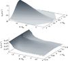 |
Fig. 8 Upper panel: 2D profile of disk radial velocity V R calculated up to the distance R = 20 Req for the Pop III star’s disk with parameters and rates given in Table 1 and Fig. 6. Contours mark the radial velocity 0.1 and 0.5 m s−1. Lower panel:2D profile of disk azimuthal velocity V ϕ calculated up to the same distance for the same model as in the upper panel. Contours mark the azimuthal velocity 2 × 10⁵, 2.5 × 10⁵, and 3 ×10⁵ m s−1. |
4.3 Models of less massive disks with disk mass-loss rate Ṁ ≤ 10−8 M⊙ yr−1 that may correspond to classical decretion disks of Be stars
The disks with a disk mass-loss rate equal to or lower than Ṁ = 10−8 M⊙ yr−1 may correspond to the classical Be stars’ disks (e.g., Carciofi & Bjorkman 2008; Krtička et al. 2011; Granada et al. 2013). The assumed parameters of the central B0-type star in this Section are introduced in Table 1. Figure 9 shows the difference in the profiles of density in the very inner region in the disk with Ṁ = 10−8 M⊙ yr−1, for the constant viscosities α = 0.1 and α =1, respectively. While the density profile for α = 0.1 is relatively smooth, the same profile for α = 1 shows the bumps (waves) that are characteristic for the models with higher density (see Sect. 4.2). Consistently, the disk base density for α = 1 is about 4–5 times lower than for α = 0.1 which corresponds to a higher radial velocity of the material outflow in the inner disk regions for higher values of α (see the models with different viscosity parameters α in Krtička et al. 2011).
The temperature structures of the disk models with Ṁ = 10−8 M⊙ yr−1, Ṁ = 10−9 M⊙ yr−1, and Ṁ = 10−10 M⊙ yr−1 up to 20 Req are plotted in Figs. 10 and 11, respectively. The maximum temperatures in the disk cores that may be generated by the viscous heating decrease with decreasing disk mass-loss rate from T ≈38 000 K in the disks with Ṁ = 10−8 M⊙ yr−1 and T ≈22 000 K in the disks with Ṁ = 10−9 M⊙ yr−1 to T ≈13 500 K in the disks with Ṁ = 10−10 M⊙ yr−1. The maximum optical depths within the same regions are τ ≈ 165, τ ≈ 20, and τ ≈ 2.2, respectively. However, forṀ ≤ 10−11 M⊙ yr−1, the disk optical depth is τ < 0.5 throughout the disk and the contribution of the viscosity to the temperature structure becomes negligible due to low disk density (lower panelof Fig. 11).
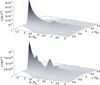 |
Fig. 9 Upper panel: 2D graph of the density of a converged model of a circumstellar viscous outflowing disk of a critically rotating B0-type star in the very inner region up to 5 stellar radii, corresponding to the disk mass-loss rate Ṁ = 10−8 M⊙ yr−1, with the constant viscosity parameter α = α0 = 0.1. The sonic point radius is in this case approximately 2.5 × 10⁴ Req and the density profile is relatively smooth. The contours mark the density values (from lower to higher) 2.5 × 10⁻⁸, 5 × 10⁻⁸, 10−7, 1.5 × 10⁻⁷, 2 × 10⁻⁷ [kg m −3], and so on, with a constant increment of 0.5 × 10⁻⁷ kg m−3. Lower panel:same graph, but with the viscosity coefficient α = α0 = 1. The density profile shows significant roughly periodic waves that occur in the case of a viscosity parameter α ≳ 0.5. The contours mark the density levels (from lower to higher) 2.5 × 10⁻⁸, 5 × 10⁻⁸, 7.5 × 10⁻⁸ and 10−7 [kg m −3]. |
5 Discussion
To test the assumption of heat equilibrium (neglecting the advection term; see Sect. 2.1), we compared the energy efficiency of external and internal sources for the disk models with Ṁ ≥ 10−6 M⊙ yr−1 (the highestexamined mass loss rates) in the following way: we quantified the radiative energy density of the stellar irradiation that impinges the disk on one side and the excess of energy density generated in the disk (kinetic energy due to the radial outflow plus the energy produced by pressure and viscosity) on the other side. The ratio of energy densities of the external irradiation to the internal sources in the model is approximately 2 orders of magnitude at the base of the disk while it approaches 3 orders of magnitude at the radius 10 Req. Obviously, in the models with lower Ṁ this ratio is higher. This comparison shows that it is not necessary to solve full energy equation to obtain the disk temperature.
Our 2D calculations of the disk-core temperature structure are based on a diffusion approximation within the optically thick domain of the disk, where the optical depth τ ≥ 2∕3, and include the contribution of heating generated by viscous friction. In the surrounding optically thin environment we calculate the temperature assuming a local thermodynamic equilibrium of the gas with the impinging stellar irradiation, including the effects of radiative loss in the optically thin approximation accounting for heavier elements (see Sect. 2.3), while neglecting the contribution of the viscous heating. We calculate self-consistently the evolution of the gas-dynamic and thermal structure of the disk within each time-step of the convergence of our time-dependent 2D models.
Similar disk models provided by, for example, Carciofi & Bjorkman (2008) or Sigut et al. (2009) employ NLTE radiative codes for the calculations of the optically thin disk temperature structure. They however use fixed hydrodynamic distribution of the disk gas, calculated prior to their NLTE models, and do not take into account the viscous friction in the core of the disk. On the other hand we take into account only the free electrons produced by ionization of hydrogen, and do not include bound-bound opacities.
Comparing the basic results of our calculations with published models, we see that the viscous heat effect begins to occur near the disk equatorial plane in the models with Ṁ = 10−10 M⊙ yr−1. The total effects of calculated viscous heat are in accordance with Lee et al. (1991) who found the domination of viscous heat generation rate over the irradiative heating rate only when Ṁ ≳ 10−5 M⊙ yr−1, regarding the vertically integrated viscous heat. For example, in the model of the Pop III star (see Table 1) with Ṁ = 10−6 M⊙ yr−1, where in the distance 1.5 Req the parameters a2 ≈ 109 m2 s−2, Ω = 7.2 × 10⁻⁶ s−1, and Σ ≈ 2.5 × 10⁵ kg m−2, we obtain  while the vertically integrated Fvis(R) ≈ 2 × 10⁸ W m−2 (the latter value is in fact even lower because we assumed here for simplicity the maximum disk core temperature 80 000 K within the whole vertical disk profile, while in reality the temperature vertically decreases). The disk base temperatures T0 ≈ 17 500 K and T0 ≈ 21 000 K in the models for Ṁ ≥ 10−9 M⊙ yr−1 in Sects. 4.2 and 4.3, respectively, correspond to approximately 70% of the stellar effective temperature ⟨Teff⟩ = 25 000 K and ⟨Teff⟩ = 30 000 K. This agrees with the calculations of Carciofi & Bjorkman (2008), for example, who found approximately T0 ∕⟨Teff⟩≈ 0.7 within the nearly isothermal solution of Keplerian viscous disk with the disk mass-loss rate Ṁ = 5 × 10⁻¹¹ M⊙ yr−1. The reason why the disk base temperature is lower than the mean effective stellar temperature is the self-shadowing of the star itself due to the stellar oblateness and equatorial darkening together with the self-shadowing of the optically thick gas in the inner disk region (Kurfürst 2015). Unlike Carciofi & Bjorkman (2008), we have not obtained a similar radial temperature profile, that is, a rapid temperature decrease to approx. 0.4 Teff at the radius R ≈ (3–4) Req followed by its increase to approx. 0.6 Teff at the radius R ≈ 5 Req in the disk midplane, which results from inclusion of the optically thin radiative equilibrium in a significantlyrarefied gas at larger distance. Sigut et al. (2009) derive the disk base temperature T0 = 13 500 K in a circumstellar viscous disk of Be star γ Cas with ⟨Teff⟩≈ 25 000 K. Several different density models of Sigut et al. (2009) with ρ0 = 10−9 kg m−3, ρ0 = 5 × 10⁻⁹ kg m−3 and ρ0 = 5 × 10⁻⁸ kg m−3 (noting that the disk mass-loss rate Ṁ = 10−11 M⊙ yr−1 roughly corresponds to ρ0 = 10−8 kg m−3), respectively, show, in the 2D temperaturedistributions of the γ Cas disk, the development of a cool region near the equatorial plane with steep vertical temperature gradients. The vertical temperature profiles in those models range approximately from 10 000 K in the disk midplane to the maximum 15 000 K in the model with highest density and approximately from 8000 K in the disk midplane to a maximum of 15 000 K in the model with lowest density, considering the radial domain up to 5 stellar radii. In our model with similar parameters (lower panel of Fig. 11), the disk vertical temperature profile varies within the range (10 000 K–12 000 K), but only in the very short radial region up to 1–2 stellar radii. However, for Ṁ = 10−11 M⊙ yr−1 our calculation is less relevant, since we do not take into account the optically thin radiative equilibrium in the relatively very low-density gas. Another question refers to the behavior of the models of B0 star disks with Ṁ = 10−10 M⊙ yr−1 and Ṁ = 10−9 M⊙ yr−1 when taking into account the NLTE calculations.
We have also fitted the models to examine the radial profiles of the disk midplane density ρeq ~ Rn in the final stationary state. Avoiding the regions with irregularities, we found the slopes of ρeq in the models of very dense disks with Ṁ = 10−6 M⊙ yr−1 corresponding to the slope parameter n between 2.85 and 3.0 (where the usual analytical solution gives the value 3.5 – see Sect. 2.4) in the region between approximately R = 6 Req and R = 20 Req. The slope parameter steepens to 4.0 in the region between approximately R = 30 Req and R = 50 Req, and the slope parameter stabilizes at approximately 3.2 in the region above the distance R ≥ 100 Req. For the less massive disks with Ṁ ≤ 10−8 M⊙ yr−1 the value of the same slope parameter within the same region is approximately 3.125. This agrees with observational results of Klement et al. (2017), who determine the values of the disk midplane density slope parameter between approximately 3.0 and 3.5 for the Be stars’ disks that are in a steady state. They also predict that disks with this parameter higher than 3.5 should correspond to disks that are in the process of formation, and that disks with this parameter lower than 3 are in the process of dissipation; the variations of the values of the slope parameter in the case of very massive disks indicate that these processes occur up to a certain distance (see Sect. 4.2).
The occurrence of the more or less irregular instabilities (density waves) in the models with Ṁ ≥ 10−7 M⊙ yr−1 (or with very high α parameter) roughly corresponds to cases of the convection development due to the steep radiative gradient (see Fig. 5). In regards to this point, our current calculations do not confirm either the violation of the Richardson criterion due to the rotation-driven instabilities (see, e.g., Maeder 2009, p. 294), or that these perturbations seem to be associated with turbulence generated by hydrodynamic (or WKB) density waves (Balbus 2003, 2011). We regard these instabilities as “viscous instabilities” caused by development of pressure bumps in the region near the base of the disk (Pinilla et al. 2012; Dullemond & Penzlin 2018). The idea of a viscous disk that may become dynamically unstable and even lead to the formation of concentric rings was also suggested by Wünsch et al. (2005). However, although the driving mechanisms of the instabilities may be, in the referred papers, different (nor are they are mathematically analyzed in detail), all the authors employ the initial infinitesimally small bump or wiggle in pressure (viscosity ordiffusion) to describe the process analytically within the perturbation theory. From disk theory (e.g., Pringle 1981; Frank et al. 2002), as well as from Eqs. (1)–(4) with use of Eq. (20), it follows that ν(R)Σ(R) = const. During the numerical convergence, the “initial perturbation” (given by the difference between the approximate initial state and the final converged state) relaxes in cases where the ν(R)Σ(R) product is relatively small while in the case of high values of the product the perturbations permanently propagate as a referred “viscous instability”. The detailed analysis of the effects of time-dependent perturbations and their distribution and evolution within the disk will be the subject of future work.
This process may also be provoked by mutual dependence of density, viscosity, and temperature (see, e.g., Figs. 4–6) when the decrease in temperature causes the decrease in density and viscous friction (and vice versa) in the inner part of the disk, which allows the material to fall back. However, the determination of the mechanism as well as the frequency of these perturbations will need to be the subject of further detailed studies (we cannot even actually rule out the effects of numerical artefacts caused by a number of mutually entangled calculations with extreme values of variables).
The nature of sgB[e] stars’ disks is an open question. There remains even a possibility of the existence of a system of rings of high-density material in the surroundings of these objects, containing gas and dust (see, e.g., Kraus et al. 2013). The formation mechanism of such a disk (or ring structure) is also unclear. We know about at least two sgB[e] candidates for rapid rotators with the rotation velocity reaching a substantial part of the critical velocity: the stars LHA 115-S 23 (Zickgraf 2000; Kraus et al. 2008) and LHA 115-S 65, both in the Small Magellanic Cloud (Kraus et al. 2010). As another example of this type of objects we may consider the Galactic eccentric binary system GG Car with a circumbinary ring, where one of the possible scenarios refers to the primary component as a classical Be star during the previous evolution of the system (Kraus et al. 2013).
Our models may provide significant corroboration of some aspects of a viscous decretion disk scenario. The performed results may, for example, confirm an agreement of the behavior of the instabilities in the theoretical models with the observed dissipation curve of time-variable dissipating disks. This provides a tool to improve an estimate of the disk viscosity parameter α and of the disk mass-loss rate Ṁ (cf., Carciofi et al. 2012, who conclude that higher values of α parameter result from turbulent viscosity induced by disk instability). We may expect also a kind of observational consequence in case of very high temperatures in the cores of very dense disks (see Sect. 4.2). Even if the cores are shielded by colder upper layers, the total radiative emission on lower frequencies should be significant. The turbulent instabilities may also lead to the enhancement of the magnetic field by a dynamo effect.
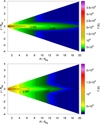 |
Fig. 10 Upper panel: color map of the temperature distribution in the inner part (up to 20 stellar equatorial radii) of the circumstellar outflowing disk of a critically rotating star with the same parameters as in Fig. 9 (Ṁ = 10−8 M⊙ yr−1, α = α0 = 0.1). The region of increased temperature generated by the viscous heating near the disk midplane extends in this case to a distance of approximately 20 Req. The contours mark the temperature levels 3000 K, 5000 K, 10 000 K, 20 000 K (and 35 000 K at the base of the disk). Lower panel: color map of the temperature distribution in the inner part (up to 20 Req) of the circumstellar outflowing disk of a critically rotating star with the same parameters as in Fig. 9, with the disk mass-loss rate Ṁ = 10−9 M⊙ yr−1, with the constant viscosity parameter α = α0 = 0.1. The region of increased temperature generated by the viscous heating near the disk midplane is significant to a distance of approximately 15 Req. The contours mark the temperature levels 2000 K, 3000 K, 5000 K, 10 000 K (and 20 000 K at the base of the disk). |
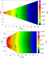 |
Fig. 11 Upper panel: color map of the temperature distribution in the inner part (up to 20 Req) of the circumstellar outflowing disk of a critically rotating star with the same stellar parameters as in Fig. 9, with the disk mass-loss rate Ṁ = 10−10 M⊙ yr−1, with the constant viscosity parameter α = α0 = 0.1. The strip of increased temperature generated by the viscous heating begins to be visible near the disk midplane. The contours mark the temperature levels 2000 K, 3000 K, 5000 K, 10 000 K (and 12 000 K at the base of the disk). Lower panel: color map of the temperature distribution in the very inner part (up to 5 stellar equatorial radii) of the circumstellar outflowing disk of a critically rotating star with the same stellar parameters as in Fig. 9, corresponding however to a disk mass-loss rate Ṁ = 10−11 M⊙ yr−1, with a constant viscosity parameter α = α0 = 0.1. The strip of increased temperature near the disk midplane generated by the viscous heating for this Ṁ disappears. The contours mark the temperature levels 5000 K, 8000 K, 10 000 K, 11 000 K, and 12 000 K. |
6 Summary and conclusions
We calculated axisymmetric, 2D, time-dependent models of circumstellar outflowing disks of critically or near-critically rotating stars in the radial-vertical plane. We developed for this purpose two types of our own numerical Eulerian hydrodynamic code that employ full Navier-Stokes viscosity: the operator-split finite volume algorithm for (relatively) smooth hydrodynamic calculations, and the unsplit finite volume algorithm (based on the Roe’s method) for the calculations of problems with sharp discontinuities and/or high Mach numbers. Furthermore, we calculated most of the performed models using both methods to compare the obtained numeric results. Our 2D models of the self-consistently calculated time-dependent density-velocity structure performed in the disk R-z (R-θ) plane employ the effects of impinging stellar irradiation of the rotationally oblate star and the internal viscous heating of the disk matter.
The models of very dense viscous disks with Ṁ > 10−8 M⊙ yr−1, which may correspond to disk or disk-like environments of Pop III stars or sgB[e] stars, show large strips of high density, optical depth and temperature that are generated by the viscosity, extending to a significant distance. Consequently, the calculations point to the existence of the convective zones in the models with Ṁ ≥ 10−7 M⊙ yr−1 that may affect the disk behavior (see Lee et al. 1991); namely they may alter the temperature and therefore the density profile and may provoke the enhancement of instabilities.
The models of the disks with the lower disk mass-loss rates, which may correspond to classical Be star disks, show less pronounced viscous-heated disk midplane strips which disappear for Ṁ < 10−10 M⊙ yr−1. The higher values of theα parameter of viscosity and/or high mass-loss rates lead to unstable disk behavior, producing waves or bumps in the inner disk region that consistently occur in the profiles of density, pressure, radial velocity, optical depth, and temperature.
The fundamental computational problem is the enormous ratio of the disk vertical scale height to the radial extent of the disk which represents several orders of magnitude within a distance of a few stellar radii from the central star. To overcome this problem, wedeveloped a specific non-orthogonal “flaring disk” grid (see Sect. 3 and Appendix A for the detailed mathematical description). However, we are still not able to model the self-consistent 2D global disk density and thermal structure significantly above the sonic point radius.
The models of disks of Pop III stars where we assume the enormous disk mass-loss rates (e.g., Marigo et al. 2001) may contribute to a better understanding of the rate of supply of interstellar space with gas as well as with radiation generated in the disks due to viscosity heating. The nature and structure of disks around sgB[e] stars (at least some of them) might be explained by the viscous disk model. The spectroscopic analyses reveal the Keplerian rotation velocity of the observed disk or rings. Many computations are still needed, however, to explain the origin and evolution of the suggested ring structure where no radial flow has been detected so far (Kraus et al. 2013). Is a structure of the concentric rings that may extend up to hundreds of stellar radii a result of stellar pulsations or sub-critical rotation with high α viscosity parameter? Taking into account the high disk mass-loss rates and therefore the high densities and optical depths in the inner disks, there appears to be (in the case of viscous disk models) a substantial contribution of viscous heating in these regions. However, the high densities produce an intensive radiative shielding in the inner disk, providing thus the possibility for a neutral hydrogen occurrence in a narrow strip near the transition from an optically thin to optically thick zone. We prove the existence of convective zones in the disks with Ṁ ≥ 10−7 M⊙ yr−1. Such zones can be relatively extended; for example, they appear in the radial range (2–14) Req in the disk with Ṁ = 10−6 M⊙ yr−1.
Acknowledgements
Access to computing and storage facilities owned by parties and projects contributing to the National Grid Infrastructure MetaCentrum, provided under the programme “Projects of Large Infrastructure for Research, Development, and Innovations” (LM2010005) is appreciated. This work was supported by the grant GA ČR 16-01116S.
Appendix A Flaring disk coordinate system
A.1 Basic transformation equations
We introduce the unique coordinate system that fits the geometry of circumstellar disks, taking into account the axisymmetricity and the vertical hydrostatic equilibrium as well as the “flaring disk” geometry. The inclusion of the flaring angle causes major difficulties of numerical schemes based on standard cylindrical coordinates. To avoid the geometrical discrepancy, we developed a new computational grid, and we call it the flaring disk coordinate system.
Figure A.1 illustrates the system in radial-vertical (R-θ) plane. The radial and azimuthal coordinates are identical with standard cylindrical coordinate system, and we thus denote them R and ϕ. The third coordinate θ is defined asthe spherical angle calculated in positive and negative direction from the equatorial plane. Transformation equations from the flaring into Cartesian coordinates are
 (A.1)
(A.1)
Transformation equations of the unit basis vectors (cf. the notation and basic principles introduced in Arfken & Weber 2005) from Cartesian to the flaring disk coordinates are
 (A.2)
(A.2)
The inverse transformation of the unit basis vectors is
 (A.3)
(A.3)
In the flaring disk coordinate system all the basis vectors are non-constant, and their directions vary in dependence on azimuthal and flaring angle. Angular and time derivatives of the unit basis vectors, covariant metric tensor gij for coordinates R, ϕ, θ, respectively, and the transformation Jacobian J from the Cartesian to the flaring disk coordinate system, are
![Mathematical equation: \begin{equation*} \begin{aligned} \frac{\partial\hat{\vec{R}}}{\partial{\phi}} & = \hat{\vec{\phi}},\\ \frac{\partial\hat{\vec{R}}}{\partial{\theta}} & =0,\\ \frac{\partial\hat{\vec{R}}}{\partial t} & =\hat{\vec{\phi}}\dot{\phi}, \end{aligned}\quad \begin{aligned} \frac{\partial\hat{\vec\phi}}{\partial\phi} & =-\hat{\vec{R}},\\ \frac{\partial\hat{\vec{\phi}}}{\partial{\theta}} & =0,\\ \frac{\partial\hat{\vec{\phi}}}{\partial t} & =-\hat{\vec{R}}\dot{\phi}, \end{aligned}\quad \begin{aligned} \frac{\partial\hat{\vec{\theta}}}{\partial\phi} & =-\hat{\vec{\phi}}\sin\theta,\\ \frac{\partial\hat{\vec{\theta}}}{\partial\theta} & =-\frac{\hat{\vec{R}}+\hat{\vec{\theta}}\sin\theta}{\cos\theta},\\ \frac{\partial\hat{\vec{\theta}}}{\partial t} & =-\frac{\hat{\vec{R}}\dot{\theta}}{\cos\theta} -\hat{\vec{\phi}}\dot{\phi}\sin\theta-\hat{\vec{\theta}}\dot{\theta}\tan\theta, \end{aligned}\quad \begin{aligned} g_{ij}= \begin{pmatrix}\dfrac{1}{\cos^2\theta} & 0 & \dfrac{R\sin\theta}{\cos^3\theta}\\[8pt] 0 & R^2 & 0 \\[2pt] \dfrac{R\sin\theta}{\cos^3\theta} & 0 & \dfrac{R^2}{\cos^4\theta} \end{pmatrix},\quad J=\frac{R^2}{\cos^2\theta}. \end{aligned} \end{equation*}](/articles/aa/full_html/2018/05/aa31300-17/aa31300-17-eq76.png) (A.4)
(A.4)
A.2 Basic differential operators
Gradient of a scalar function f = f(R, ϕ, θ) is
 (A.5)
(A.5)
The gradient of an arbitrary vector field A(R, ϕ, θ) for coordinates R, ϕ, θ, respectively, is the matrix ∇A whose elements are
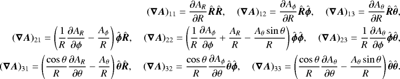 (A.6)
(A.6)
Divergence of an arbitrary vector field A(R, ϕ, θ), defined as adot product of the gradient vector (Eq. (A.5)) and an arbitrary vector  (with nonzero dot product of different basis vectors
  ), is
), is
![Mathematical equation: \begin{align*}\vec{\nabla}\cdot\vec{A}= \frac{1}{R}\frac{\partial}{\partial R}\left(R A_R\right)+ \frac{1}{R}\frac{\partial A_{\phi}}{\partial\phi}+ \frac{\cos\theta}{R}\frac{\partial A_{\theta}}{\partial\theta}- \frac{\sin\theta}{R}\left[ \frac{\partial}{\partial R}\left(R A_{\theta}\right)+\cos\theta\frac{\partial A_R}{\partial\theta}\right]. \end{align*}](/articles/aa/full_html/2018/05/aa31300-17/aa31300-17-eq81.png) (A.7)
(A.7)
Curl of a vector A(R, ϕ, θ) is defined as a cross product of gradient vector (Eq. (A.5)) and an arbitrary vector  where the cross products of different basis vectors are
 (A.8)
(A.8)
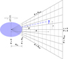 |
Fig. A.1 Schema of the flaring disk (wedge-cylindrical) coordinate system in radial-vertical (R-θ) plane. Coordinates of arbitrary point P are R, ϕ, θ. Intersection of coordinate surface |
Curl of a vector in the flaring disk system takes the form
![Mathematical equation: \begin{eqnarray*}\vec\nabla\times\vec{A}&=&\hat{\vec{R}} \left\{\frac{\tan\theta}{R}\left[\frac{\partial}{\partial R}\left(R A_{\phi}\right)-\frac{\partial A_R}{\partial\phi}\right]+ \frac{1}{R}\left(\frac{1}{\cos\theta}\frac{\partial A_{\theta}}{\partial\phi}-\frac{\partial A_{\phi}}{\partial\theta}\right)\right\}+ \hat{\vec{\phi}} \left\{\frac{\cos\theta}{R}\left[\cos\theta\frac{\partial A_R}{\partial\theta}- \frac{\partial}{\partial R}\left(R A_{\theta}\right)\right]\right\}\nonumber\\ &&+\,\hat{\vec{\theta}} \left\{\frac{1}{R\cos\theta}\left[\frac{\partial}{\partial R}\left(R A_{\phi}\right)-\frac{\partial A_R}{\partial\phi}\right]+ \frac{\sin\theta}{R}\left(\frac{1}{\cos\theta}\frac{\partial A_{\theta}}{\partial\phi}-\frac{\partial A_{\phi}}{\partial\theta}\right)\right\}. \end{eqnarray*}](/articles/aa/full_html/2018/05/aa31300-17/aa31300-17-eq84.png) (A.9)
(A.9)
The Laplacian operator in the flaring disk system becomes
 (A.10)
Volumes and surfaces
Volumes and surfaces of computational grid cells are used in the method of finite volume (see Sect. 3). The volume bounded by coordinate surfaces (the surfaces with constant coordinates R2, R1, ϕ1, ϕ2, θ1, θ2) is
 (A.11)
The areas of corresponding grid cell surfaces (where the subscripts refer to the constant surface coordinate) are
 (A.12)
A.4 Velocity and acceleration
The vectors of position r and velocity  in the flaring disk coordinates take the form
 (A.13)
We obtain the components of the vector of acceleration  by differentiation of the velocity in Eq. (A.13),
![Mathematical equation: \begin{align*}a_R=\frac{\ddot{R}+R\ddot{\theta}\tan\theta+2\dot{\theta}\,(\dot{R}+R\dot{\theta}\tan\theta)\tan\theta}{\cos^2\theta}-R\dot{\phi}^2,\quad a_{\phi}=R\ddot{\phi}+2\dot{R}\dot{\phi},\quad a_{\theta}=\frac{1}{\cos\theta}\left[\ddot{R}\tan\theta+\frac{R\ddot{\theta}+2\dot{\theta}\,(\dot{R}+R\dot{\theta}\,\tan\theta)}{\cos^2\theta}\right]. \end{align*}](/articles/aa/full_html/2018/05/aa31300-17/aa31300-17-eq91.png) (A.14)
(A.14)
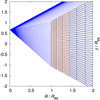 |
Fig. A.2 Schematic graph of the entirely inner part of the flaring disk grid in radial-vertical (R-θ) plane with marked ray-tracing for calculation of the disk optical depth. All the rays come from one point (from the “north” pole of a critically rotating star where Req = 1.5 R⋆). The grid cells are depicted as black lines, the blue rays intersect the vertical cell interfaces while the red lines enter the grid cells through their upper flaring interface (or the lower flaring interface for the not plotted rays that emerge from the stellar “south” pole). See Sect. A.5 for the description. |
From Eqs. (A.13) and (A.14) we express the components of the velocity vector as
 (A.15)
Following the identity dV∕dt = ∂V∕∂t +V ⋅∇V, we write the components of the vector of acceleration in terms of the velocity vector components,
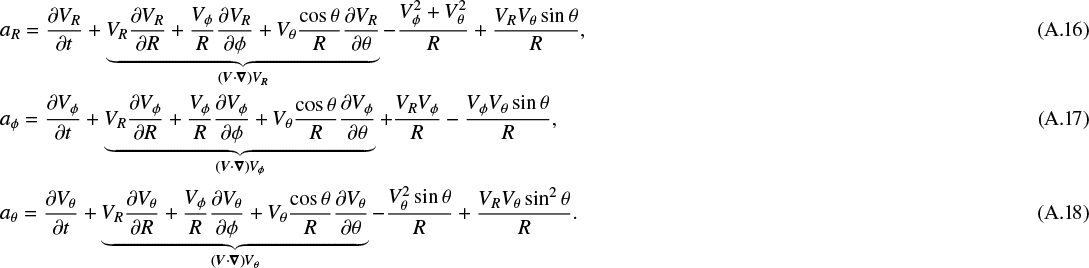
The underbraced terms on the right-hand sides of Eqs. (A.16)–(A.18) express the nonlinear advection while the other terms represent the apparent centrifugal and Coriolis accelerations (“fictitious forces”). This perfectly corresponds to a general theorem that in the classical rotating frame with constant angular velocity Ω (see, e.g., Landau & Lifshitz 1982, p. 128), the only apparent accelerations are the centrifugal and Coriolis (new apparent accelerations may occur, e.g., in general relativity).
From Eqs. (A.1) and (A.15) we express the velocity vector components V R, V ϕ, V θ in terms of the velocity vector components in standard cylindrical coordinate system, V R, cyl, V ϕ, cyl, V z, obtaining
 (A.19)
Taking into account the vertical hydrostatic balance, V z = 0, the hydrodynamic acceleration terms, Eqs. (A.16)–(A.18), become however identical to corresponding terms in standard cylindrical coordinates. Noting here that the flaring geometry of the disks together with the vertical hydrostatic equilibrium assumption are the main reasons for introducing this coordinate system, this is an important simplification of its mathematical complexity. Some small difficulties connected with the nonorthogonal flaring disk coordinate system thus mainly remain at the technical level (in the correct implementation of the grid).
A.5 Calculation of the disk optical depth
We trace the optical depth along the rays showed schematically in Fig. A.2 using the short characteristics method (we plan a more advanced calculation with large number of radiation sources on the stellar surface within the future work). We denote δ the angle of a diagonal of a computational grid cell,
 (A.20)
Denoting the radial and vertical coordinate values of intersection of the ray with vertical or “flaring disk” grid cell interface, R′ and z′ , respectively, and denoting the vertical coordinate value of intersection of the ray with “flaring disk” grid cell interface, z′′ , we may obtain the following relations,
 (A.21)
where R⋆ is the stellar polar radius. For the calculation of the optical depth (cf. Eq. (26)) we have to distinguish two cases of the δ slope in respect to the source of rays,
 (A.22)
We use thepiecewise linear interpolation of the quantity χ =κρ. The first and second case in Eq. (A.22) respectively imply,
![Mathematical equation: \begin{align*}{\mathrm{\Delta}}\tau_{i,k} = \left[\chi_{i,k}(R^{\prime},z^{\prime\prime})+\chi_{i,k}(R,z)\right]\,{\mathrm{\Delta}} s_{i,k}\,/2,\quad {\mathrm{\Delta}}\tau_{i,k} = \left[\chi_{i,k}(R_{i-1},z^{\prime})+\chi_{i,k}(R,z)\right]\,{\mathrm{\Delta}} s_{i,k}\,/2, \end{align*}](/articles/aa/full_html/2018/05/aa31300-17/aa31300-17-eq98.png) (A.23)
(A.23)
where Δτ is the increase of τ and Δs is the length of the path of the ray within one computational cell. The optical depth for each grid point i, k is then calculated as  where
where  is the linearly interpolated optical depth in points (
 ) or (
 ), according toEq. (A.22). The described principle takes into account only the optical depth tracing on one side of the disk (for therays that emerge, e.g., from the “north” stellar pole according to Fig. A.2), and for the other side of the disk the principle applies analogously.
A.6 Eigensystems of the flaring disk coordinates using the Roe’s method: adiabatic hydrodynamics
For adiabatic hydrodynamics in the flaring disk coordinate frame with the conservative variables U = (ρ, ΠR, Πϕ, Πθ, E) = (u1, …, u5) we write Eq. (40) in 3D component form (see the formalism and terminology given in, e.g., Toro 1999; Stone et al. 2008),
 (A.24)
where F, G, H are the vectors of fluxes in the R, ϕ, θ directions, respectively, and S is the vector of geometric source terms. The factors ξ = 1, ξ′ = sinθ stay at particular R, θ components of the flux F, factors η = 1, η′ = sinθ stay at particular θ, R components of the flux H, factors ζ = 1, ζ′ = sinθ stay at particular R, θ components of the geometric source term S. The explicit conservative form of the basic adiabatic hydrodynamic equations (equation of continuity, three components of momentum equation and energy equation, omitting the source terms) in the flaring disk coordinate frame is
![Mathematical equation: \begin{align} \frac{\partial\rho}{\partial t}+\frac{\partial}{\partial R}\left(\rho V^{\prime}\right)+\frac{1}{R}\frac{\partial}{\partial\phi}\left(\rho V_{\phi}\right) +\frac{\cos\theta}{R}\left[\frac{\partial}{\partial\theta}\left(\rho V_{\theta}\right)-\sin\theta\frac{\partial}{\partial\theta}\left(\rho V_R\right)\right]= -\frac{\rho V^{\prime}}{R},\\[1pt] \frac{\partial\left(\rho V_R\right)}{\partial t}+\frac{\partial}{\partial R}\left[\rho\left(V_RV^{\prime}+H\right)-E\right]+ \frac{1}{R}\frac{\partial}{\partial\phi}\left(\rho V_RV_{\phi}\right) +\frac{\cos\theta}{R}\left[\frac{\partial}{\partial\theta}\left(\rho V_RV_{\theta}\right)-\sin\theta\frac{\partial}{\partial\theta}\left(\rho V_R^2\right)\right]= -\frac{\rho V_RV^{\prime}}{R},\\[1pt] \frac{\partial\left(\rho V_{\phi}\right)}{\partial t}+\frac{\partial}{\partial R}\left(\rho V_{\phi} V^{\prime}\right)+ \frac{1}{R}\frac{\partial}{\partial\phi}\left[\rho\left(V_{\phi}^2+H\right)-E\right] +\frac{\cos\theta}{R}\left[\frac{\partial}{\partial\theta}\left(\rho V_{\phi} V_{\theta}\right)-\sin\theta\frac{\partial}{\partial\theta}\left(\rho V_RV_{\phi}\right)\right]= -\frac{\rho V_{\phi} V^{\prime}}{R},\\[1pt] \frac{\partial\left(\rho V_{\theta}\right)}{\partial t}+\frac{\partial}{\partial R}\left(\rho V_{\theta} V^{\prime}\right)+ \frac{1}{R}\frac{\partial}{\partial\phi}\left(\rho V_{\phi} V_{\theta}\right) +\frac{\cos\theta}{R}\left\{\frac{\partial}{\partial\theta}\left[\rho\left(V_{\theta}^2+H\right)-E\right]- \sin\theta\frac{\partial}{\partial\theta}\left(\rho V_R V_{\theta}\right)\right\} =-\frac{\rho V_{\theta} V^{\prime}}{R},\\[1pt] \frac{\partial E}{\partial t}+\frac{\partial}{\partial R}\left(\rho V^{\prime} H\right)+\frac{1}{R}\frac{\partial}{\partial\phi}\left(\rho V_{\phi} H\right) +\frac{\cos\theta}{R}\left[\frac{\partial}{\partial\theta}\left(\rho V_{\theta} H\right)-\sin\theta\frac{\partial}{\partial\theta}\left(\rho V_R H\right)\right]= -\frac{\rho V^{\prime} H}{R}.\end{align}](/articles/aa/full_html/2018/05/aa31300-17/aa31300-17-eq104.png)
We hereafter substitute V R−θ = V R − V θ, V θ−R = V θ − V R, V ′ = V R−θ sinθ, H is the enthalpy,  , and the velocity vector V = (V R, V ϕ, V θ). The explicit components of F, G, H, S, are
![Mathematical equation: \begin{align*}\vec{F}= \begin{bmatrix} \rho V_{R-\theta}\\[2pt]\rho V_RV_{R-\theta}+P\\[2pt]\rho V_{\phi} V_{R-\theta}\\[2pt]\rho V_{\theta} V_{R-\theta}\\[2pt](E+P)V_{R-\theta} \end{bmatrix},\quad \vec{G}= \begin{bmatrix} \rho V_{\phi}\\[2pt]\rho V_RV_{\phi}\\[2pt]\rho V_{\phi}^2+P\\[2pt]\rho V_{\phi} V_{\theta}\\[2pt](E+P)V_{\phi} \end{bmatrix},\quad \vec{H}= \begin{bmatrix} \rho V_{\theta-R}\\[2pt]\rho V_RV_{\theta-R}\\[2pt]\rho V_{\phi} V_{\theta-R}\\[2pt]\rho V_{\theta} V_{\theta-R}+P\\[2pt](E+P)V_{\theta-R} \end{bmatrix},\quad \vec{S}=-\frac{1}{R} \begin{bmatrix} \rho V_{R-\theta}\\[2pt]\rho\vec{V}V_{R-\theta}\\[2pt](E+P)V_{R-\theta} \end{bmatrix}. \end{align*}](/articles/aa/full_html/2018/05/aa31300-17/aa31300-17-eq106.png) (A.30)
(A.30)
The vectors F, G, H written in terms of the five conservative variables U = (u1, …, u5), corresponding to Eq. (40) in the flaring disk coordinates, are
![Mathematical equation: \begin{align*}\vec{F}(\vec{u}),\vec{G}(\vec{u}),\vec{H}(\vec{u}) = \begin{pmatrix} u_2-u_4^*,u_3,u_4-u_2^*\\[4pt]\dfrac{(u_2-u_4^*)u_2}{u_1}+(\gamma-1)\left[u_5-\dfrac{u_2^2+u_3^2+u_4^2}{2u_1}\right],\dfrac{u_3u_2}{u_1},\dfrac{(u_4-u_2^*)u_2}{u_1}\\[2pt] \dfrac{(u_2-u_4^*)u_3}{u_1},\dfrac{u_3^2}{u_1}+(\gamma-1)\left[u_5-\dfrac{u_2^2+u_3^2+u_4^2}{2u_1}\right],\dfrac{(u_4-u_2^*)u_3}{u_1}\\[2pt] \dfrac{(u_2-u_4^*)u_4}{u_1},\dfrac{u_3u_4}{u_1},\dfrac{(u_4-u_2^*)u_4}{u_1}+(\gamma-1)\left[u_5-\dfrac{u_2^2+u_3^2+u_4^2}{2u_1}\right]\\[2pt] \left[\gamma u_5-(\gamma-1)\dfrac{u_2^2+u_3^2+u_4^2}{2u_1}\right]\left(\dfrac{u_2-u_4^*}{u_1},\dfrac{u_3}{u_1},\dfrac{u_4-u_2^*}{u_1}\right) \end{pmatrix}, \end{align*}](/articles/aa/full_html/2018/05/aa31300-17/aa31300-17-eq107.png) (A.31)
(A.31)
where the asterisk denotes the factor sinθ staying in front of the derivative of the particular term. Equation (A.31) demonstrates the proper swapping of the corresponding components of momentum (cf., e.g., Stone et al. 2008; Skinner & Ostriker 2010).
The adiabatic conservative Jacobian matrices  ,
,  , and
, and  , where we hereafter denote μ = cosθ, written explicitly in the directionally swapped form, are
![Mathematical equation: \begin{align*}\mathbf{A_1^{\mathbf{C}}}= \begin{bmatrix} 0 & 1 & 0 &-\sin\theta & 0\\ -V_RV^{\prime}+(\gamma-1)\dfrac{V^2}{2} &-(\gamma-2)V_R+V^{\prime} &-(\gamma-1)V_{\phi} & V^{\prime\prime}-\gamma V_{\theta} & \gamma-1\\ -V_{\phi} V^{\prime} & V_{\phi} & V^{\prime} &-V_{\phi}\sin\theta & 0\\[2pt] -V_{\theta} V^{\prime} & V_{\theta} & 0 & V^{\prime}-V_{\theta}\sin\theta & 0\\ -V^{\prime} H+(\gamma-1)\dfrac{V^{\prime} V^2}{2} &-(\gamma-1)V_RV^{\prime}+H &-(\gamma-1)V_{\phi} V^{\prime} &-(\gamma-1)V_{\theta} V^{\prime}-H\sin\theta & \gamma V^{\prime} \end{bmatrix}, \end{align*}](/articles/aa/full_html/2018/05/aa31300-17/aa31300-17-eq111.png) (A.32)
(A.32)
![Mathematical equation: \begin{align*}\mathbf{A_2^{\mathbf{C}}}=\frac{1}{R} \begin{bmatrix} 0 & 0 & 1 & 0 & 0\\[2pt] -V_{\phi} V_R & V_{\phi} & V_R & 0 & 0\\ -V_{\phi}^2+(\gamma-1)\dfrac{V^2}{2} &-(\gamma-1)V_R &-(\gamma-3)V_{\phi} &-(\gamma-1)V_{\theta} & \gamma-1\\ -V_{\phi} V_{\theta} & 0& V_{\theta} & V_{\phi} & 0\\ -V_{\phi} H+(\gamma-1)\dfrac{V_{\phi} V^2}{2} &-(\gamma-1)V_RV_{\phi} &-(\gamma-1)V_{\phi}^2+H &-(\gamma-1)V_{\phi} V_{\theta} & \gamma V_{\phi} \end{bmatrix}, \end{align*}](/articles/aa/full_html/2018/05/aa31300-17/aa31300-17-eq112.png) (A.33)
(A.33)
![Mathematical equation: \begin{align*}\mathbf{A_3^{\mathbf{C}}}=\frac{\mu}{R} \begin{bmatrix} 0 &-\sin\theta & 0 & 1 & 0\\[2pt] -V_RV^{\prime\prime} & V^{\prime\prime}-V_R\sin\theta & 0 & V_R & 0\\[2pt] -V_{\phi} V^{\prime\prime} &-V_{\phi}\sin\theta & V^{\prime\prime} & V_{\phi} & 0\\ -V_{\theta} V^{\prime\prime}+(\gamma-1)\dfrac{V^2}{2} & V^{\prime}-\gamma V_R &-(\gamma-1)V_{\phi} &-(\gamma-2)V_{\theta}+V^{\prime\prime} & \gamma-1\\ -V^{\prime\prime}H+(\gamma-1)\dfrac{V^{\prime\prime}V^2}{2} &-(\gamma-1)V_RV^{\prime\prime}-H\sin\theta &-(\gamma-1)V_{\phi} V^{\prime\prime} & -(\gamma-1)V_{\theta} V^{\prime\prime}+H & \gamma V^{\prime\prime} \end{bmatrix}, \end{align*}](/articles/aa/full_html/2018/05/aa31300-17/aa31300-17-eq113.png) (A.34)
(A.34)
where we hereafter substitute V ′′ = V θ−R sinθ. The corresponding eigenvalues  , of the matrices
  ,
,  ,
,  , are
, are
 (A.35)
where a is the adiabatic speed of sound, a2 = γP∕ρ. Corresponding right eigenvectors (following the directional swapping in Eqs. (A.32) and (A.34)) are the columns of the matrices
![Mathematical equation: \begin{align*}\mathbf{R_1^{\mathbf{C}}} = \begin{pmatrix} 1 & 0 & 0 & 1 & 1\\[2pt] V_R-a & 0 & \sin\theta & V_R & V_R+a \\[2pt] V_{\phi} & 1 & 0 & V_{\phi} & V_{\phi}\\[2pt] V_{\theta} & 0 & 1 & V_{\theta} & V_{\theta}\\ H^{\prime}_{-} & V_{\phi} & \mu^2V_{\theta} & \dfrac{V^2}{2}&H^{\prime}_{+} \end{pmatrix},\,\, \mathbf{R_2^{\mathbf{C}}} = \begin{pmatrix} 1 & 0 & 1 & 0 & 1 \\[2pt] V_R & 1 & V_R & 0 & V_R \\[2pt] V_{\phi}-a & 0 & V_{\phi} & 0& V_{\phi}+a \\[2pt] V_{\theta} & 0 & V_{\theta} & 1 & V_{\theta} \\ H-V_{\phi} a & V^{\prime} & \dfrac{V^2}{2} & V^{\prime\prime} & H+V_{\phi} a \end{pmatrix},\,\, \mathbf{R_3^{\mathbf{C}}} = \begin{pmatrix} 1 & 1 & 0 & 0 & 1 \\[2pt] V_R & V_R & 1 & 0 & V_R \\[2pt] V_{\phi} & V_{\phi} & 0 & 1 & V_{\phi} \\[2pt] V_{\theta}-a & V_{\theta} & \sin\theta & 0 & V_{\theta}+a \\ H^{\prime\prime}_{-} & \dfrac{V^2}{2} & \mu^2V_R & V_{\phi} & H^{\prime\prime}_{+} \end{pmatrix}, \end{align*}](/articles/aa/full_html/2018/05/aa31300-17/aa31300-17-eq119.png) (A.36)
(A.36)
where  ,
,  ,
,  and
and  . The corresponding left eigenvectors are the rows of the matrices
![Mathematical equation: \begin{align*}\mathbf{L_1^{\mathbf{C}}} = \begin{bmatrix} \dfrac{(\gamma-1)V^2/2+V^{\prime} a}{2a^2} &-\dfrac{(\gamma-1)V^{\prime}+a}{2a^2} &-\dfrac{(\gamma-1)V_{\phi}}{2a^2} &-\dfrac{(\gamma-1)V^{\prime\prime}-a\sin\theta}{2a^2}&\dfrac{\gamma-1}{2a^2}\\[7pt] -V_{\phi} & 0 & 1 & 0 & 0 \\[1pt] -V_{\theta} & 0 & 0 & 1 & 0 \\ 1-\dfrac{(\gamma-1)V^2}{2a^2} & \dfrac{(\gamma-1)V^{\prime}}{a^2} & \dfrac{(\gamma-1)V_{\phi}}{a^2} & \dfrac{(\gamma-1)V^{\prime\prime}}{a^2} & -\dfrac{\gamma-1}{a^2} \\ \dfrac{(\gamma-1)V^2/2-V^{\prime} a}{2a^2} &-\dfrac{(\gamma-1)V^{\prime}-a}{2a^2} &-\dfrac{(\gamma-1)V_{\phi}}{2a^2} &-\dfrac{(\gamma-1)V^{\prime\prime}+a\sin\theta}{2a^2} & \dfrac{\gamma-1}{2a^2} \end{bmatrix}, \end{align*}](/articles/aa/full_html/2018/05/aa31300-17/aa31300-17-eq124.png) (A.37)
(A.37)
![Mathematical equation: \begin{align*}\mathbf{L_2^{\mathbf{C}}} = \begin{bmatrix} \dfrac{(\gamma-1)V^2/2+V_{\phi} a}{2a^2} &-\dfrac{(\gamma-1)V^{\prime}}{2a^2} &-\dfrac{(\gamma-1)V_{\phi}+a}{2a^2} &-\dfrac{(\gamma-1)V^{\prime\prime}}{2a^2} & \dfrac{\gamma-1}{2a^2} \\[7pt] -V_R & 1 & 0 & 0 & 0\\ 1-\dfrac{(\gamma-1)V^2}{2a^2} & \dfrac{(\gamma-1)V^{\prime}}{a^2} & \dfrac{(\gamma-1)V_{\phi}}{a^2} & \dfrac{(\gamma-1)V^{\prime\prime}}{a^2}& -\dfrac{\gamma-1}{a^2} \\[7pt] -V_{\theta} & 0 & 0 & 1 & 0\\ \dfrac{(\gamma-1)V^2/2-V_{\phi} a}{2a^2}&-\dfrac{(\gamma-1)V^{\prime}}{2a^2}&-\dfrac{(\gamma-1)V_{\phi}-a}{2a^2} &-\dfrac{(\gamma-1)V^{\prime\prime}}{2a^2} & \dfrac{\gamma-1}{2a^2} \end{bmatrix}, \end{align*}](/articles/aa/full_html/2018/05/aa31300-17/aa31300-17-eq125.png) (A.38)
(A.38)
![Mathematical equation: \begin{align*}\mathbf{L_3^{\mathbf{C}}} = \begin{bmatrix} \dfrac{(\gamma-1)V^2/2+V^{\prime\prime}a}{2a^2} &-\dfrac{(\gamma-1)V^{\prime}-a\sin\theta}{2a^2} &-\dfrac{(\gamma-1)V_{\phi}}{2a^2} &-\dfrac{(\gamma-1)V^{\prime\prime}+a}{2a^2} & \dfrac{\gamma-1}{2a^2}\\ 1-\dfrac{(\gamma-1)V^2}{2a^2} & \dfrac{(\gamma-1)V^{\prime}}{a^2} & \dfrac{(\gamma-1)V_{\phi}}{a^2} & \dfrac{(\gamma-1)V^{\prime\prime}}{a^2} &-\dfrac{\gamma-1}{a^2}\\[7pt] -V_R & 1 & 0 & 0 & 0 \\[1pt] -V_{\phi} & 0 & 1 & 0 & 0 \\ \dfrac{(\gamma-1)V^2/2-V^{\prime\prime}a}{2a^2} &-\dfrac{(\gamma-1)V^{\prime}+a\sin\theta}{2a^2} & -\dfrac{(\gamma-1)V_{\phi}}{2a^2} &-\dfrac{(\gamma-1)V^{\prime\prime}-a}{2a^2} & \dfrac{\gamma-1}{2a^2} \end{bmatrix}. \end{align*}](/articles/aa/full_html/2018/05/aa31300-17/aa31300-17-eq126.png) (A.39)
(A.39)
The same set of adiabatic equations (A.25)–(A.29) expressed in terms of primitive variables W = (ρ, V R, V ϕ, V θ, P) = (w1, …, w5) takes the form
![Mathematical equation: \begin{align} \frac{\partial\rho}{\partial t}+\rho\left[\frac{\partial V^{\prime}}{\partial R}+\frac{1}{R}\frac{\partial V_{\phi}}{\partial\phi}+ \frac{\mu}{R}\left(\frac{\partial V_{\theta}}{\partial\theta}-\sin\theta\frac{\partial V_R}{\partial\theta}\right)\right] +V^{\prime}\frac{\partial\rho}{\partial R}+\frac{V_{\phi}}{R}\frac{\partial\rho}{\partial\phi}+ \frac{\mu}{R}V^{\prime\prime}\frac{\partial\rho}{\partial\theta}=-\frac{\rho V^{\prime}}{R},\\[1pt] \frac{\partial V_R}{\partial t}+V^{\prime}\frac{\partial V_R}{\partial R}+\frac{V_{\phi}}{R}\frac{\partial V_R}{\partial\phi}+ \frac{\mu}{R}V^{\prime\prime}\frac{\partial V_R}{\partial\theta}+\frac{1}{\rho}\frac{\partial P}{\partial R}=0,\\[1pt] \frac{\partial V_{\phi}}{\partial t}+V^{\prime}\frac{\partial V_{\phi}}{\partial R}+\frac{V_{\phi}}{R}\frac{\partial V_{\phi}}{\partial \phi}+ \frac{\mu}{R}V^{\prime\prime}\frac{\partial V_{\phi}}{\partial \theta}+\frac{1}{\rho R}\frac{\partial P}{\partial\phi}=0,\\[1pt] \frac{\partial V_{\theta}}{\partial t}+V^{\prime}\frac{\partial V_{\theta}}{\partial R}+\frac{V_{\phi}}{R}\frac{\partial V_{\theta}}{\partial \phi}+ \frac{\mu}{R}\left(V^{\prime\prime}\frac{\partial V_{\theta}}{\partial\theta}+\frac{1}{\rho}\frac{\partial P}{\partial\theta}\right)=0,\\[1pt] \frac{\partial P}{\partial t}+\gamma P\left[\frac{\partial V^{\prime}}{\partial R}+\frac{1}{R}\frac{\partial V_{\phi}}{\partial\phi}+ \frac{\mu}{R}\left(\frac{\partial V_{\theta}}{\partial\theta}-\sin\theta\frac{\partial V_R}{\partial\theta}\right)\right] +(\gamma V)^{\prime}\frac{\partial P}{\partial R}+\frac{V_{\phi}}{R}\frac{\partial P}{\partial\phi}+ \frac{\mu}{R}(\gamma V)^{\prime\prime}\frac{\partial P}{\partial\theta}=-\frac{\gamma PV^{\prime}}{R}, \end{align}](/articles/aa/full_html/2018/05/aa31300-17/aa31300-17-eq127.png)
where we substitute the expressions  ,
,  . The adiabatic primitive Roe matrices
  ,
,  , and
, and  , become
![Mathematical equation: \begin{align*}\mathbf{A_1^{\mathbf{P}}} = \begin{bmatrix} V^{\prime} & \rho & 0 &-\rho\sin\theta & 0 \\ 0 & V^{\prime} & 0 & 0 & \dfrac{1}{\rho} \\ 0 & 0 & V^{\prime} & 0 & 0 \\[1pt] 0 & 0 & 0 & V^{\prime} & 0 \\[1pt] 0 & \rho a^2 & 0 &-\rho a^2\sin\theta & \left(\gamma V\right)^{\prime} \end{bmatrix},\quad \mathbf{A_2^{\mathbf{P}}} = \frac{1}{R} \begin{pmatrix} V_{\phi} & 0 & \rho & 0 & 0 \\[1pt] 0 & V_{\phi} & 0 & 0 & 0 \\0 & 0 & V_{\phi} & 0 & \dfrac{1}{\rho}\\0 & 0 & 0 & V_{\phi} & 0 \\[1pt] 0 & 0 & \rho a^2 & 0 & V_{\phi} \end{pmatrix},\quad \mathbf{A_3^{\mathbf{P}}} = \frac{\mu}{R} \begin{bmatrix} V^{\prime\prime} &-\rho\sin\theta & 0 & \rho & 0 \\[1pt] 0 & V^{\prime\prime} & 0 & 0 & 0 \\[1pt] 0 & 0 & V^{\prime\prime} & 0 & 0 \\ 0 & 0 & 0 & V^{\prime\prime} & \dfrac{1}{\rho} \\ 0 &-\rho a^2\sin\theta & 0 & \rho a^2 & \left(\gamma V\right)^{\prime\prime} \end{bmatrix}. \end{align*}](/articles/aa/full_html/2018/05/aa31300-17/aa31300-17-eq133.png) (A.45)
(A.45)
The corresponding eigenvalues  , of the matrices
  ,
,  ,
,  , are
, are
 (A.46)
The corresponding right eigenvectors (following the directional swapping in Eq. (A.45)) are the columns of the matrices
![Mathematical equation: \begin{align*}\mathbf{R_1^{\mathbf{P}}} = \begin{pmatrix} 1 & 1 & 0 & 0 & 1 \\-\dfrac{a}{\rho} & 0 & 0 & \sin\theta & \dfrac{a}{\rho} \\ 0 & 0 & 1 & 0 & 0 \\[1pt] 0 & 0 & 0 & 1 & 0 \\[1pt] a^2 & 0 & 0 & 0 & a^2 \end{pmatrix},\quad \mathbf{R_2^{\mathbf{P}}} = \begin{pmatrix} 1 & 1 & 0 & 0 & 1 \\[1pt] 0 & 0 & 1 & 0 & 0 \\-\dfrac{a}{\rho} & 0 & 0 & 0 & \dfrac{a}{\rho} \\ 0 & 0 & 0 &1 & 0 \\[1pt] a^2 & 0 & 0 & 0 & a^2 \end{pmatrix},\quad \mathbf{R_3^{\mathbf{P}}} = \begin{pmatrix} 1 & 1 & 0 & 0 & 1 \\[1pt] 0 & 0 & 0 & 1 & 0 \\[1pt] 0 & 0 & 1 & 0 & 0 \\-\dfrac{a}{\rho} & 0 & 0 & \sin\theta & \dfrac{a}{\rho} \\ a^2 & 0 & 0 & 0 & a^2 \end{pmatrix}, \end{align*}](/articles/aa/full_html/2018/05/aa31300-17/aa31300-17-eq139.png) (A.47)
(A.47)
while the corresponding left eigenvectors are the rows of the matrices
![Mathematical equation: \begin{align*}\mathbf{L_1^{\mathbf{P}}} = \begin{pmatrix} 0 &-\dfrac{\rho}{2a} & 0 & \dfrac{\rho\sin\theta}{2a} & \dfrac{1}{2a^2} \\ 1 & 0 & 0 & 0 &-\dfrac{1}{a^2} \\ 0 & 0 & 1 & 0 & 0 \\[1pt] 0 & 0 & 0 & 1 & 0 \\ 0 & \dfrac{\rho}{2a} & 0 &-\dfrac{\rho\sin\theta}{2a} & \dfrac{1}{2a^2} \end{pmatrix},\quad \mathbf{L_2^{\mathbf{P}}} = \begin{pmatrix} 0 & 0 &-\dfrac{\rho}{2a} & 0 & \dfrac{1}{2a^2} \\ 1 & 0 & 0 & 0 &-\dfrac{1}{a^2}\\0 & 1 & 0 & 0 & 0 \\[1pt] 0 & 0 & 0 & 1 & 0 \\ 0 & 0 & \dfrac{\rho}{2a} & 0 & \dfrac{1}{2a^2} \end{pmatrix},\quad \mathbf{L_3^{\mathbf{P}}} = \begin{pmatrix} 0 & \dfrac{\rho\sin\theta}{2a} & 0 &-\dfrac{\rho}{2a} & \dfrac{1}{2a^2} \\ 1 & 0 & 0 & 0 &-\dfrac{1}{a^2} \\ 0 & 0 & 1 & 0 & 0 \\[1pt] 0 & 1 & 0 & 0 & 0 \\ 0 &-\dfrac{\rho\sin\theta}{2a} & 0 & \dfrac{\rho}{2a} & \dfrac{1}{2a^2} \end{pmatrix}. \end{align*}](/articles/aa/full_html/2018/05/aa31300-17/aa31300-17-eq140.png) (A.48)
(A.48)
The explicit forms of the vectors of adiabatic conservative and primitive geometric source terms SC and SP are
![Mathematical equation: \begin{align*} \vec{S}^{\mathbf{C}}=-\frac{1}{R} \begin{pmatrix} \rho V^{\prime}\\[1pt]\rho\vec{V}V^{\prime}\\[1pt]\rho V^{\prime} H \end{pmatrix},\quad \vec{S}^{\mathbf{P}} = -\frac{1}{R} \begin{pmatrix} \rho V^{\prime}\\[1pt]\vec{0}\\[1pt]\rho a^2 V^{\prime} \end{pmatrix}. \end{align*}](/articles/aa/full_html/2018/05/aa31300-17/aa31300-17-eq141.png) (A.49)
(A.49)
A.7 Eigensystems of the flaring disk coordinates using the Roe’s method: isothermal hydrodynamics
For isothermal hydrodynamics in the flaring disk coordinate frame with the conservative variables U = (ρ, ΠR, Πϕ, Πθ) = (u1, …, u4) we write Eq. (40) in 3D component form (see the formalism and terminology given in, e.g., Toro 1999; Stone et al. 2008; Skinner & Ostriker 2010),
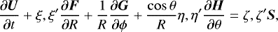 (A.50)
where F, G, H are the vectors of fluxes in the R, ϕ, θ directions, respectively, and S is the vector of geometric source terms. The factors ξ = 1, ξ′ = sinθ stay at particular R, θ components of the flux F, factors η = 1, η′ = sinθ stay at particular θ, R components of the flux H and factors ζ = 1, ζ′ = sinθ stay at particular R, θ components of the geometric source term S. We consistently use in this Section the following substitutions: V R−θ = V R − V θ, V θ−R = V θ − V R, V ′ = V R−θ sinθ, V ′′ = V θ−R sinθ, μ = cosθ.
The explicit conservative form of the basic isothermal hydrodynamic equations (equation of continuity and three components of momentum equation, omitting the source terms) in the flaring disk coordinate frame is
![Mathematical equation: \begin{align} \frac{\partial\rho}{\partial t}+\frac{\partial}{\partial R}\left(\rho V^{\prime}\right)+\frac{1}{R}\frac{\partial}{\partial\phi}\left(\rho V_{\phi}\right)+ \frac{\mu}{R}\left[\frac{\partial}{\partial\theta}\left(\rho V_{\theta}\right)-\sin\theta\frac{\partial}{\partial\theta}\left(\rho v_R\right)\right]=-\frac{\rho V^{\prime}}{R},\\[1pt] \frac{\partial}{\partial t}\left(\rho V_R\right)+\frac{\partial}{\partial R}\left[\rho\left(V_RV^{\prime}+C^2\right)\right]+\frac{1}{R}\frac{\partial}{\partial\phi}\left(\rho V_RV_{\phi}\right)+ \frac{\mu}{R}\left[\frac{\partial}{\partial\theta}\left(\rho V_RV_{\theta}\right)-\sin\theta\frac{\partial}{\partial\theta}\left(\rho V_R^2\right)\right]=-\frac{\rho V_RV^{\prime}}{R},\\[1pt] \frac{\partial}{\partial t}\left(\rho V_{\phi}\right)+\frac{\partial}{\partial R}\left(\rho V_{\phi} V^{\prime}\right)+\frac{1}{R}\frac{\partial}{\partial\phi}\left[\rho\left(V_{\phi}^2+C^2\right)\right]+ \frac{\mu}{R}\left[\frac{\partial}{\partial\theta}\left(\rho V_{\phi} V_{\theta}\right)-\sin\theta\frac{\partial}{\partial\theta}\left(\rho V_RV_{\phi}\right)\right]= -\frac{\rho V_{\phi} V^{\prime}}{R},\\[1pt] \frac{\partial}{\partial t}\left(\rho V_{\theta}\right)+\frac{\partial}{\partial R}\left(\rho V_{\theta} V^{\prime}\right)+\frac{1}{R}\frac{\partial}{\partial\phi}\left(\rho V_{\phi} V_{\theta}\right)+ \frac{\mu}{R}\left\{\frac{\partial}{\partial\theta}\left[\rho\left(V_{\theta}^2+C^2\right)\right]-\sin\theta\frac{\partial}{\partial\theta}\left(\rho V_RV_{\theta}\right)\right\}= -\frac{\rho V_{\theta} V^{\prime}}{R},\end{align}](/articles/aa/full_html/2018/05/aa31300-17/aa31300-17-eq143.png)
where we denote the isothermal speed of sound, C, in this Section. The explicit components Fiso, Giso, Hiso, Siso, are
![Mathematical equation: \begin{align*}\vec{F}_{\mathbf{iso}} = \begin{pmatrix} \rho V_{R-\theta}\\[2pt]\rho V_RV_{R-\theta}+C^2\rho\\[2pt]\rho V_{\phi} V_{R-\theta}\\[2pt]\rho V_{\theta} V_{R-\theta} \end{pmatrix},\quad \vec{G}_{\mathbf{iso}} = \begin{pmatrix} \rho V_{\phi}\\[2pt]\rho V_R V_{\phi}\\[2pt]\rho V_{\phi}^2+C^2\rho\\[2pt]\rho V_{\phi} V_{\theta} \end{pmatrix},\quad \vec{H}_{\mathbf{iso}} = \begin{pmatrix} \rho V_{\theta-R}\\[2pt]\rho V_RV_{\theta-R}\\[2pt]\rho V_{\phi} V_{\theta-R}\\[2pt]\rho V_{\theta} V_{\theta-R}+C^2\rho \end{pmatrix},\quad \vec{S}_{\mathbf{iso}} = -\frac{1}{R} \begin{pmatrix} \rho V_{R-\theta}\\[2pt]\rho\vec{V}V_{R-\theta} \end{pmatrix}. \end{align*}](/articles/aa/full_html/2018/05/aa31300-17/aa31300-17-eq144.png) (A.55)
(A.55)
The vectors Fiso, Giso, Hiso, written in terms of the four conservative variables U = (u1, …, u4), corresponding to Eq. (40) in the flaring disk coordinates, are
![Mathematical equation: \begin{align*}\vec{F}_{\mathbf{iso}}(\vec{u}) = \begin{bmatrix} u_2-u_4^*\\[1pt]\dfrac{u_2(u_2-u_4^*)}{u_1}+C^2u_1\\[1pt]\dfrac{u_3(u_2-u_4^*)}{u_1}\\[1pt]\dfrac{u_4(u_2-u_4^*)}{u_1} \end{bmatrix},\quad \vec{G}_{\mathbf{iso}}(\vec{u}) = \begin{pmatrix} u_3\\[3pt]\dfrac{u_3u_2}{u_1}\\[1pt]\dfrac{u_3^2}{u_1}+C^2u_1\\[1pt]\dfrac{u_3u_4}{u_1} \end{pmatrix},\quad \vec{H}_{\mathbf{iso}}(\vec{u}) = \begin{bmatrix} u_4-u_2^*\\[1pt]\dfrac{u_2(u_4-u_2^*)}{u_1}\\[1pt]\dfrac{u_3(u_4-u_2^*)}{u_1}\\[1pt]\dfrac{u_4(u_4-u_2^*)}{u_1}+C^2u_1 \end{bmatrix}, \end{align*}](/articles/aa/full_html/2018/05/aa31300-17/aa31300-17-eq145.png) (A.56)
(A.56)
where the asterisk denotes the factor sinθ staying in front of the derivative of the particular term.
The isothermal conservative Jacobian matrices  ,
,  ,
,  , and the vector
  , are
, are
![Mathematical equation: \begin{align*}\mathbf{A_{1,{\mathbf{iso}}}^{\mathbf{C}}} = \begin{pmatrix} 0&1&0&-\sin\theta\\[1pt]-V_RV^{\prime}+C^2&V_R+V^{\prime}&0&-V_R\sin\theta\\[1pt] -V_{\phi} V^{\prime}&V_{\phi}&V^{\prime}&-V_{\phi}\sin\theta\\[1pt]-V_{\theta} V^{\prime}&V_{\theta}&0&V^{\prime}-V_{\theta}\sin\theta \end{pmatrix},\quad \mathbf{A_{2,{\mathbf{iso}}}^{\mathbf{C}}} = \frac{1}{R} \begin{pmatrix} 0&0&1&0\\[1pt]-V_{\phi} V_R&V_{\phi}&V_R&0\\[1pt]-V_{\phi}^2+C^2&0&2V_{\phi}&0\\[1pt]-V_{\phi} V_{\theta}&0&V_{\theta}&V_{\phi} \end{pmatrix}, \end{align*}](/articles/aa/full_html/2018/05/aa31300-17/aa31300-17-eq150.png) (A.57)
(A.57)
![Mathematical equation: \begin{align*}\mathbf{A_{3,{\mathbf{iso}}}^{\mathbf{C}}} = \frac{\mu}{R} \begin{pmatrix} 0&-\sin\theta&0&1\\[1pt]-V_R V^{\prime\prime}&V^{\prime\prime}-V_R\sin\theta&0&V_R\\[1pt] -V_{\phi} V^{\prime\prime}&-V_{\phi}\sin\theta&V^{\prime\prime}&V_{\phi}\\[1pt]-V_{\theta} V^{\prime\prime}+C^2&-V_{\theta}\sin\theta&0&V_{\theta}+V^{\prime\prime} \end{pmatrix},\quad \vec{S}_{\mathbf{iso}}^{\mathbf{C}}=-\frac{1}{R} \begin{pmatrix} \rho V^{\prime}\\[1pt]\rho\vec{V}V^{\prime} \end{pmatrix}. \end{align*}](/articles/aa/full_html/2018/05/aa31300-17/aa31300-17-eq151.png) (A.58)
(A.58)
The corresponding eigenvalues  , of the matrices
  ,
,  ,
,  , are
, are
 (A.59)
The corresponding right eigenvectors (following the directional swapping of Eqs. (A.57) and (A.58)) are the columns of the matrices
![Mathematical equation: \begin{align*}\mathbf{R_{1,{\mathbf{iso}}}^{\mathbf{C}}} = \begin{pmatrix} 1&0&0&1\\[1pt] V_R-C&0&\sin\theta&V_R+C\\[1pt] V_{\phi}&1&0&V_{\phi}\\[1pt] V_{\theta}&0&1&V_{\theta} \end{pmatrix},\quad \mathbf{R_{2,{\mathbf{iso}}}^{\mathbf{C}}} = \begin{pmatrix} 1&0&0&1\\[1pt] V_R&0&1&V_R\\[1pt] V_{\phi}-C&0&0&V_{\phi}+C\\[1pt] V_{\theta}&1&0&V_{\theta} \end{pmatrix},\quad \mathbf{R_{3,{\mathbf{iso}}}^{\mathbf{C}}} = \begin{pmatrix} 1&0&0&1\\[1pt] V_R&0&1&V_R\\[1pt] V_{\phi}&1&0&V_{\phi}\\[1pt] V_{\theta}-C&0&\sin\theta&V_{\theta}+C \end{pmatrix}. \end{align*}](/articles/aa/full_html/2018/05/aa31300-17/aa31300-17-eq157.png) (A.60)
(A.60)
The corresponding left eigenvectors are the rows of the matrices,
![Mathematical equation: \begin{align*}\mathbf{L_{1,{\mathbf{iso}}}^{\mathbf{C}}} = \begin{pmatrix} \dfrac{1+V^{\prime}/C}{2}&-\dfrac{1}{2C}&0&\dfrac{\sin\theta}{2C}\\[7pt] -V_{\phi}&0&1&0\\[1pt] -V_{\theta}&0&0&1\\\dfrac{1-V^{\prime}/C}{2}&\dfrac{1}{2C}&0&-\dfrac{\sin\theta}{2C} \end{pmatrix},\quad \mathbf{L_{2,{\mathbf{iso}}}^{\mathbf{C}}} = \begin{pmatrix} \dfrac{1+V_{\phi}/C}{2}&0&-\dfrac{1}{2C}&0\\[7pt] -V_{\theta}&0&0&1\\[1pt] -V_R&1&0&0\\[1pt]\dfrac{1-V_{\phi}/C}{2}&0&\dfrac{1}{2C}&0 \end{pmatrix},\quad \mathbf{L_{3,{\mathbf{iso}}}^{\mathbf{C}}} = \begin{pmatrix} \dfrac{1+V^{\prime\prime}/C}{2}&\dfrac{\sin\theta}{2C}&0&-\dfrac{1}{2C}\\[7pt]-V_{\phi}&0&1&0\\[1pt] -V_R&1&0&0\\ \dfrac{1-V^{\prime\prime}/C}{2}&-\dfrac{\sin\theta}{2C}&0&\dfrac{1}{2C} \end{pmatrix}. \end{align*}](/articles/aa/full_html/2018/05/aa31300-17/aa31300-17-eq158.png) (A.61)
(A.61)
The same set of isothermal hydrodynamic Eqs. (A.51)–(A.54) expressed in terms of primitive variables W = (ρ, V R, V ϕ, V θ) = (w1, …, w4) takes the form
![Mathematical equation: \begin{align}\frac{\partial\rho}{\partial t}+\rho\left[\frac{\partial V^{\prime}}{\partial R}+\frac{1}{R}\frac{\partial V_{\phi}}{\partial\phi}+ \frac{\mu}{R}\left(\frac{\partial V_{\theta}}{\partial\theta}-\sin\theta\frac{\partial V_R}{\partial\theta}\right)\right]+ V^{\prime}\frac{\partial\rho}{\partial R}+\frac{V_{\phi}}{R}\frac{\partial\rho}{\partial\phi}+ \frac{\mu}{R}V^{\prime\prime}\frac{\partial\rho}{\partial\theta}=-\frac{\rho V^{\prime}}{R},\\[1pt] \frac{\partial V_R}{\partial t}+V^{\prime}\frac{\partial V_R}{\partial R}+\frac{V_{\phi}}{R}\frac{\partial V_R}{\partial\phi}+ \frac{\mu}{R}V^{\prime\prime}\frac{\partial V_R}{\partial\theta}+\frac{C^2}{\rho}\frac{\partial\rho}{\partial R}=0,\\[1pt] \frac{\partial V_{\phi}}{\partial t}+V^{\prime}\frac{\partial V_{\phi}}{\partial R}+\frac{V_{\phi}}{R}\frac{\partial V_{\phi}}{\partial\phi}+ \frac{\mu}{R}V^{\prime\prime}\frac{\partial V_{\phi}}{\partial\theta}+\frac{C^2}{\rho R}\frac{\partial\rho}{\partial\phi}=0,\\[1pt] \frac{\partial V_{\theta}}{\partial t}+V^{\prime}\frac{\partial V_{\theta}}{\partial R}+\frac{V_{\phi}}{R}\frac{\partial V_{\theta}}{\partial\phi}+ \frac{\mu}{R}V^{\prime\prime}\frac{\partial V_{\theta}}{\partial\theta}+\frac{\mu}{R}\frac{C^2}{\rho}\frac{\partial\rho}{\partial\theta}=0.\end{align}](/articles/aa/full_html/2018/05/aa31300-17/aa31300-17-eq159.png)
The corresponding matrices  and the vector
  in terms of the primitive variables W become
![Mathematical equation: \begin{align*}\mathbf{A_{1,{\mathbf{iso}}}^{\mathbf{P}}} = \begin{pmatrix} V^{\prime}&\rho&0&-\rho\sin\theta\\\dfrac{C^2}{\rho}&V^{\prime}&0&0\\[7pt] 0&0&V^{\prime}&0\\[1pt] 0&0&0&V^{\prime} \end{pmatrix},\,\, \mathbf{A_{2,{\mathbf{iso}}}^{\mathbf{P}}} = \frac{1}{R} \begin{pmatrix} V_{\phi}&0&\rho&0\\0&V_{\phi}&0&0\\[1pt]\dfrac{C^2}{\rho}&0&V_{\phi}&0\\[1pt] 0&0&0&V_{\phi} \end{pmatrix},\,\, \mathbf{A_{3,{\mathbf{iso}}}^{\mathbf{P}}} = \frac{\mu}{R} \begin{pmatrix} V^{\prime\prime}&-\rho\sin\theta&0&\rho\\0&V^{\prime\prime}&0&0\\0&0&V^{\prime\prime}&0\\\dfrac{C^2}{\rho}&0&0&V^{\prime\prime} \end{pmatrix},\,\, \vec{S}_{\mathbf{iso}}^{\mathbf{P}} = -\frac{1}{R} \begin{pmatrix} \rho V^{\prime}\\\vec{0} \end{pmatrix}. \end{align*}](/articles/aa/full_html/2018/05/aa31300-17/aa31300-17-eq162.png) (A.66)
(A.66)
The corresponding eigenvalues  , of the matrices
  ,
,  ,
,  , are
, are
 (A.67)
The corresponding right eigenvectors (following the directional swapping of Eqs. (A.57) and (A.58)) are the columnsof the matrices
![Mathematical equation: \begin{align*}\mathbf{R_{1,{\mathbf{iso}}}^{\mathbf{P}}} = \begin{pmatrix} 1&0&0&1\\-\dfrac{C}{\rho}&\sin\theta&0&\dfrac{C}{\rho}\\[7pt] 0&0&1&0\\[1pt] 0&1&0&0 \end{pmatrix},\quad \mathbf{R_{2,{\mathbf{iso}}}^{\mathbf{P}}} = \begin{pmatrix} 1&0&0&1\\[1pt] 0&1&0&0\\-\dfrac{C}{\rho}&0&0&\dfrac{C}{\rho}\\[7pt]0&0&1&0 \end{pmatrix},\quad \mathbf{R_{3,{\mathbf{iso}}}^{\mathbf{P}}} = \begin{pmatrix} 1&0&0&1\\[1pt] 0&0&1&0\\[1pt] 0&1&0&0\\-\dfrac{C}{\rho}&0&\sin\theta&\dfrac{C}{\rho} \end{pmatrix}. \end{align*}](/articles/aa/full_html/2018/05/aa31300-17/aa31300-17-eq168.png) (A.68)
(A.68)
The corresponding left eigenvectors are the rows of the matrices
![Mathematical equation: \begin{align*}\mathbf{L_{1,{\mathbf{iso}}}^{\mathbf{P}}} = \begin{pmatrix} \dfrac{1}{2}&-\dfrac{\rho}{2C}&0&\dfrac{\rho\sin\theta}{2C}\\[7pt] 0&0&1&0\\[1pt] 0&0&0&1\\\dfrac{1}{2}&\dfrac{\rho}{2C}&0&-\dfrac{\rho\sin\theta}{2C} \end{pmatrix},\quad \mathbf{L_{2,{\mathbf{iso}}}^{\mathbf{P}}} = \begin{pmatrix} \dfrac{1}{2}&0&-\dfrac{\rho}{2C}&0\\[7pt] 0&1&0&0\\[1pt] 0&0&0&1\\\dfrac{1}{2}&0&\dfrac{\rho}{2C}&0 \end{pmatrix},\quad \mathbf{L_{3,{\mathbf{iso}}}^{\mathbf{P}}} = \begin{pmatrix} \dfrac{1}{2}&\dfrac{\rho\sin\theta}{2C}&0&-\dfrac{\rho}{2C}\\[7pt] 0&0&1&0\\[1pt] 0&1&0&0\\ \dfrac{1}{2}&-\dfrac{\rho\sin\theta}{2C}&0&\dfrac{\rho}{2C} \end{pmatrix}. \end{align*}](/articles/aa/full_html/2018/05/aa31300-17/aa31300-17-eq169.png) (A.69)
(A.69)
A.8 Computation of the time increment of the unsplit algorithm in the flaring coordinates
The principle of the computation of time increment is common for both eigensystems in both types of variables: we compute a new timestep Δ t using the pre-defined CFL number C0 ≤ 1∕2, satisfying the cell-centered stability condition
![Mathematical equation: \begin{align*}{\mathrm{\Delta}} t=C_0\,\text{min}\left[\frac{{\mathrm{\Delta}} R}{\text{max}(\lambda_1)},\frac{R\,{\mathrm{\Delta}}\phi}{\text{max}(\lambda_2)}, \frac{(R/\mu)\,{\mathrm{\Delta}}\theta}{\text{max}(\lambda_3)}\right], \end{align*}](/articles/aa/full_html/2018/05/aa31300-17/aa31300-17-eq170.png) (A.70)
(A.70)
where we however describe the complete 3D form. The denominators max (λα) in Eq. (A.70) denote either the eigenvalues |V α| + a from Eqs. (A.35) and (A.46) for adiabatic hydrodynamics or the eigenvalues |V α | + C from Eqs. (A.59) and (A.67) for isothermal hydrodynamics that are already evaluated using the updated quantities (cf. Stone et al. 2008; Skinner & Ostriker 2010).
References
- Arfken, G. B.,& Weber, H. J. 2005, Mathematical Methods for Physicists, 6th edn. (Amsterdam; Boston: Elsevier) [Google Scholar]
- Balbus, S. A. 2003, ARA&A, 41, 555 [NASA ADS] [CrossRef] [Google Scholar]
- Balbus, S. A. 2011, Nature, 470, 475 [NASA ADS] [CrossRef] [Google Scholar]
- Caramana, E. J., Shashkov, M. J., & Whalen, P. P. 1998, J. Comput. Phys., 144, 70 [NASA ADS] [CrossRef] [Google Scholar]
- Carciofi, A. C. 2011, in IAU Symposium, 272, Active OB Stars: Structure, Evolution, Mass Loss, and Critical Limits, eds. C. Neiner, G. Wade, G. Meynet,& G. Peters (Cambridge University Press), 325 [Google Scholar]
- Carciofi, A. C., & Bjorkman, J. E. 2008, ApJ, 684, 1374 [NASA ADS] [CrossRef] [EDP Sciences] [Google Scholar]
- Carciofi, A. C., Bjorkman, J. E., Otero, S. A., et al. 2012, ApJ, 744, L15 [NASA ADS] [CrossRef] [Google Scholar]
- Carlsson, M., & Leenaarts, J. 2012, A&A, 539, A39 [NASA ADS] [CrossRef] [EDP Sciences] [Google Scholar]
- Chung, T. J. 2002, Computational Fluid Dynamics, (Cambridge, UK: Cambridge University Press), 1036 [Google Scholar]
- Davies, B., Oudmaijer, R. D., & Vink, J. S. 2005, A&A, 439, 1107 [NASA ADS] [CrossRef] [EDP Sciences] [Google Scholar]
- Dullemond, C. P., & Penzlin, A. B. T. 2018, A&A, 609, A50 [NASA ADS] [CrossRef] [EDP Sciences] [Google Scholar]
- Ekström, S., Meynet, G., Maeder, A., & Barblan, F. 2008, A&A, 478, 467 [NASA ADS] [CrossRef] [EDP Sciences] [Google Scholar]
- Feldmeier, A. 1995, A&A, 299, 523 [NASA ADS] [Google Scholar]
- Frank, J., King, A., & Raine, D. J. 2002, Accretion Power in Astrophysics: Third Edition (Cambridge University Press), 398 [Google Scholar]
- Granada, A., Ekström, S., Georgy, C., et al. 2013, A&A, 553, A25 [NASA ADS] [CrossRef] [EDP Sciences] [Google Scholar]
- Guinan, E. F., & Hayes, D. P. 1984, ApJ, 287, L39 [NASA ADS] [CrossRef] [Google Scholar]
- Harmanec, P. 1988, Bull. Astron. Inst. Czechoslov., 39, 329 [Google Scholar]
- Heger, A., & Langer, N. 1998, A&A, 334, 210 [NASA ADS] [Google Scholar]
- Heyrovský, D. 2007, ApJ, 656, 483 [NASA ADS] [CrossRef] [Google Scholar]
- Hillier, D. J. 2006, in ASP Conf. Ser., 355, Stars with the B[e] Phenomenon, eds. M. Kraus, & A. S. Miroshnichenko, 39 [Google Scholar]
- Hirsch, C. 1989, Numerical Computation of Internal and External Flows, 1, Fundamentals of Numerical Discretization (John Wiley & Sons) [Google Scholar]
- Kee, N. D., Owocki, S., & Sundqvist, J. O. 2016, MNRAS, 458, 2323 [NASA ADS] [CrossRef] [Google Scholar]
- Klement, R., Carciofi, A. C., Rivinius, T., et al. 2017, A&A, 601, A74 [NASA ADS] [CrossRef] [EDP Sciences] [Google Scholar]
- Kraus, M., Borges Fernandes, M., & de Araújo, F. X. 2007, A&A, 463, 627 [NASA ADS] [CrossRef] [EDP Sciences] [Google Scholar]
- Kraus, M., Borges Fernandes, M., Kubát, J., & de Araújo, F. X. 2008, A&A, 487, 697 [NASA ADS] [CrossRef] [EDP Sciences] [Google Scholar]
- Kraus, M., Borges Fernandes, M., & de Araújo, F. X. 2010, A&A, 517, A30 [NASA ADS] [CrossRef] [EDP Sciences] [Google Scholar]
- Kraus, M., Oksala, M. E., Nickeler, D. H., et al. 2013, A&A, 549, A28 [NASA ADS] [CrossRef] [EDP Sciences] [Google Scholar]
- Krtička, J., Owocki, S. P., & Meynet, G. 2011, A&A, 527, A84 [NASA ADS] [CrossRef] [EDP Sciences] [Google Scholar]
- Krtička, J., Kurfürst, P., & Krtičková, I. 2015, A&A, 573, A20 [NASA ADS] [CrossRef] [EDP Sciences] [Google Scholar]
- Kurfürst, P. 2012, in IAU Symp., 282, From Interacting Binaries to Exoplanets: Essential Modeling Tools, eds. M. T. Richards & I. Hubeny, 257 [Google Scholar]
- Kurfürst, P. 2015, Ph.D. thesis, Masaryk University, Brno, Czech Republic [Google Scholar]
- Kurfürst, P., & Krtička, J. 2012, in ASP Conf. Ser., 464, Circumstellar Dynamics at High Resolution, eds. A. C. Carciofi, & T. Rivinius, 223 [Google Scholar]
- Kurfürst, P., Feldmeier, A., & Krtička, J. 2014, A&A, 569, A23 [NASA ADS] [CrossRef] [EDP Sciences] [Google Scholar]
- Kurfürst, P., Feldmeier, A., & Krtička, J. 2017, in ASP Conf. Ser., 508, The B[e] Phenomenon: Forty Years of Studies, eds. A. Miroshnichenko, S. Zharikov, D. Korčáková, & M. Wolf, 17 [NASA ADS] [Google Scholar]
- Landau, L. D., & Lifshitz, E. M. 1982, Mechanics: 1 (Course of Theoretical Physics S) (Butterworth-) [Google Scholar]
- Lee, U., Osaki, Y., & Saio, H. 1991, MNRAS, 250, 432 [NASA ADS] [CrossRef] [Google Scholar]
- Leenaarts, J., Carlsson, M., Hansteen, V., & Gudiksen, B. V. 2011, A&A, 530, A124 [NASA ADS] [CrossRef] [EDP Sciences] [Google Scholar]
- LeVeque, R. J., Mihalas, D., Dorfi, E. A., & Müller, E. 1998, Computational Methods for Astrophysical Fluid Flow (Springer Verlag) [Google Scholar]
- Maeder, A. 1999, A&A, 347, 185 [NASA ADS] [Google Scholar]
- Maeder, A. 2009, Physics, Formation and Evolution of Rotating Stars (Springer Verlag) [Google Scholar]
- Marigo, P., Girardi, L., Chiosi, C., & Wood, P. R. 2001, A&A, 371, 152 [NASA ADS] [CrossRef] [EDP Sciences] [Google Scholar]
- McGill, M. A., Sigut, T. A. A., & Jones, C. E. 2011, ApJ, 743, 111 [NASA ADS] [CrossRef] [Google Scholar]
- Meynet, G., Ekström, S., & Maeder, A. 2006, A&A, 447, 623 [NASA ADS] [CrossRef] [EDP Sciences] [Google Scholar]
- Mihalas, D. 1978, Stellar Atmospheres, 2nd edn. (W. H. Freeman and Co.) [Google Scholar]
- Mihalas, D., & Mihalas, B. W. 1984, Foundations of Radiation Hydrodynamics (Oxford University Press) [Google Scholar]
- Norman, M. L., & Winkler, K.-H. A. 1986, in NATO Advanced Science Institutes (ASI) Series C, 188, eds. K.-H. A. Winkler & M. L. Norman, 187 [Google Scholar]
- Okazaki, A. T. 1991, PASJ, 43, 75 [NASA ADS] [Google Scholar]
- Okazaki, A. T. 2001, PASJ, 53, 119 [NASA ADS] [CrossRef] [Google Scholar]
- Okazaki, A. T. 2007, in ASP Conf. Ser., 361, Active OB-Stars: Laboratories for Stellare and Circumstellar Physics, eds. A. T. Okazaki, S. P. Owocki, & S. Stefl, 230 [Google Scholar]
- Penna, R. F., Sa̧dowski, A., Kulkarni, A. K., & Narayan, R. 2013, MNRAS, 428, 2255 [NASA ADS] [CrossRef] [Google Scholar]
- Pinilla, P., Birnstiel, T., Ricci, L., et al. 2012, A&A, 538, A114 [NASA ADS] [CrossRef] [EDP Sciences] [Google Scholar]
- Pringle, J. E. 1981, ARA&A, 19, 137 [NASA ADS] [CrossRef] [Google Scholar]
- Rivinius, T., Carciofi, A. C., & Martayan, C. 2013, A&ARv, 21, 69 [Google Scholar]
- Roe, P. L. 1981, J. Comput. Phys., 43, 357 [Google Scholar]
- Rosner, R., Tucker, W. H., & Vaiana, G. S. 1978, ApJ, 220, 643 [NASA ADS] [CrossRef] [Google Scholar]
- Schulte-Ladbeck, R. E., Clayton, G. C., Hillier, D. J., Harries, T. J., & Howarth, I. D. 1994, ApJ, 429, 846 [NASA ADS] [CrossRef] [Google Scholar]
- Schulz, W. D. 1964, J. Math. Phys., 5, 133 [NASA ADS] [CrossRef] [Google Scholar]
- Schwarzschild, M. 1958, Structure and Evolution of the Stars (Princeton University Press) [Google Scholar]
- Shakura, N. I., & Sunyaev, R. A. 1973, A&A, 24, 337 [NASA ADS] [Google Scholar]
- Shu, F. H. 1992, The Physics of Astrophysics. II: Gas Dynamics (Mill Valley, CA: University Science Books) [Google Scholar]
- Sigut, T. A. A., & Jones, C. E. 2007, ApJ, 668, 481 [NASA ADS] [CrossRef] [Google Scholar]
- Sigut, T. A. A., McGill, M. A., & Jones, C. E. 2009, ApJ, 699, 1973 [NASA ADS] [CrossRef] [Google Scholar]
- Skinner, M. A., & Ostriker, E. C. 2010, ApJS, 188, 290 [NASA ADS] [CrossRef] [Google Scholar]
- Smak, J. 1989, Acta Astron., 39, 201 [NASA ADS] [Google Scholar]
- Štefl, S., Baade, D., Rivinius, T., et al. 2003, A&A, 402, 253 [NASA ADS] [CrossRef] [EDP Sciences] [Google Scholar]
- Stone, J. M., & Norman, M. L. 1992, ApJS, 80, 753 [Google Scholar]
- Stone, J. M., Gardiner, T. A., Teuben, P., Hawley, J. F., & Simon, J. B. 2008, ApJS, 178, 137 [NASA ADS] [CrossRef] [Google Scholar]
- Thé, P. S., de Winter, D., & Pérez, M. R. 1994, A&AS, 104 [Google Scholar]
- Toro, E. F. 1999, Riemann Solvers and Numerical Methods for Fluid Dynamics: A Practical Introduction, 2nd edn. (Springer Verlag) [CrossRef] [Google Scholar]
- Townsend, R. H. D., Owocki, S. P., & Howarth, I. D. 2004, MNRAS, 350, 189 [Google Scholar]
- van Hamme, W. 1993, AJ, 106, 2096 [NASA ADS] [CrossRef] [Google Scholar]
- von Neumann, J., & Richtmyer, R. D. 1950, J. Appl. Phys., 21, 232 [NASA ADS] [CrossRef] [MathSciNet] [Google Scholar]
- von Zeipel, H. 1924, MNRAS, 84, 665 [NASA ADS] [CrossRef] [Google Scholar]
- Wade, R. A., & Rucinski, S. M. 1985, A&AS, 60, 471 [NASA ADS] [Google Scholar]
- Wünsch, R., Klahr, H., & Różyczka, M. 2005, MNRAS, 362, 361 [NASA ADS] [CrossRef] [Google Scholar]
- Zel’dovich, Ya. B., & Raizer, Yu. P. 1967, Physics of Shock Waves and High-Temperature Hydrodynamic Phenomena (New York: Academic Press) [Google Scholar]
- Zickgraf, F. 2000, in ASP Conf. Ser., 214, IAU Colloq. 175: The Be Phenomenon in Early-Type Stars, eds. M. A. Smith, H. F. Henrichs, & J. Fabregat, 26 [Google Scholar]
- Zickgraf, F.-J. 1998, in Astrophys. Space Sci. Lib., 233, B[e] Stars, eds. A. M. Hubert, & C. Jaschek, 1 [NASA ADS] [Google Scholar]
All Tables
Stellar parameters for B0-type star (Harmanec 1988, see also Kurfürst et al. 2014) and for typical Pop III star (e.g., Marigo et al. 2001) used in the models.
All Figures
|
Fig. 1 Schema of the geometry of the disk irradiation by a central star. The disk “surface” element d S (with centralpoint B) is impinged by the stellar radiation coming along the line-of-sight vector d from the stellar surface element dS⋆ (with centralpoint A). Here α is the angle between the position vector of the point A and the vector d, β′ is the angle between normal vector ν of the surface element dS and the line-of-sight vector d, β = π∕2 − β′, and γ is the angle between normals of the surface element dS and of the equatorial plane. The idea is adapted from Smak (1989). |
| In the text | |
|
Fig. 2 Schema of the rotationally oblate star with polar radius R⋆, equatorial radius Req, and stellar surface element dS⋆ whose position vector is r (with magnitude r). The vector geff is normal to the stellar surface element dS⋆. The angle ϵ denotes the deviation between the vectors ggrav (which is antiparallel to vector r) and g eff. |
| In the text | |
|
Fig. 3 Snapshot of the density wave propagating in the distance R ≈ 55Req in the converging 2D model of the isothermal outflowing disk (cf. the disk-forming density wave in 1D models in Kurfürst et al. 2014), calculated in the R-z (R-θ) plane. The elapsed time since the start of the simulation is approximately 80 days. The parameters of the critically rotating B0-type parent star are introduced in Table 1. The sonic point is beyond the displayed domain (Rs ≈ 5.5 × 10² Req). The model is calculated using the flaring grid whose prescription is given in Appendix A. The initial disk midplane density is determined by the stellar mass-loss rate Ṁ = 10−9 M⊙ yr−1 and the viscosity is parameterized as α = α0 = 0.025 (Penna et al. 2013). |
| In the text | |
|
Fig. 4 2D graph of the density of the converged model of a circumstellar viscous outflowing disk of a (near) critically rotating star in the very inner region up to 5 stellar radii, corresponding to the disk mass-loss rate Ṁ = 10−6 M⊙ yr−1, with the constant viscosity parameter α = α0 = 0.1. The parameters of the star correspond to average parameters of Pop III stars (see Table 1) or sgB[e] stars (e.g., Kraus et al. 2007). The sonic point is in this case at a distance of approximately 2 × 10⁴ Req. The density profile shows in this case irregular bumps in the very inner disk region. The contours mark the density levels (from lower to higher) 10−9, 10−8, 10−7, 10−6, 2.5 × 10⁻⁶, 5 × 10⁻⁶ [kg m −3], and so on, with a constant increment of 2.5 × 10⁻⁶ kg m−3. |
| In the text | |
|
Fig. 5 Upper panel: color map of the profile of the optical depth in the inner part (up to 20 stellar equatorial radii) of the dense circumstellar outflowing disk of a (near) critically rotating star with the same parameters as in Fig. 4. The optical depth is calculated using the method described in Appendix A.5. The outer black contour traces the optical depth level τ = 0.75 that is calculated along the line-of-sight from the stellar pole (described as “along the ray” in the figure legend), while the blue contour traces the same optical depth calculated along the vertical (z axis) direction. The inner black contour traces the optical depth level τ = 2500 that is calculated along the line-of-sight from the stellar pole. Lower panel: map of the convective zones with ∇rad > ∇ad on the same scale. The large zones refer to the disk mass-loss rate Ṁ = 10−6 M⊙ yr−1 while the small wings near the disk base refer to Ṁ = 10−7 M⊙ yr−1. |
| In the text | |
|
Fig. 6 Upperpanel: color map of the temperature distribution in the very inner part (up to 5 stellar equatorial radii) of the dense circumstellar outflowing disk of a (near) critically rotating star with the same parameters as in Fig. 4. The region of significantly increased temperature near the disk midplane is generated by the viscous heating. The contours mark the temperature levels 5000 K, 10 000 K, 20 000 K, 50 000 K and 80 000 K. Lower panel: as in the upper panel, in theinner part up to 20 stellar equatorial radii. The strip of highly increased temperature near the disk midplane is generated by the viscous heating. The contours mark the temperature levels 3000 K, 10 000 K and 50 000 K. |
| In the text | |
|
Fig. 7 Upper panel: as in Fig. 6, up to the intermediate distance of 50 stellar equatorial radii. The near-equatorial strip of enhanced temperature exceeds in this case the distance 50 Req. The contours mark the temperature levels 1000 K, 2000 K, 5000 K and 10 000 K. Lower panel: color map of the temperature distribution in the very inner part (up to 5 stellar equatorial radii) of the dense circumstellar outflowing disk of a (near) critically rotating star with the same parametersas in Fig. 4, however, the parameterized disk mass-loss rate is in this case Ṁ = 10−7 M⊙ yr−1. The region of increased temperature generated by the viscous heating near the disk midplaneis in this case significantly reduced and extends up to only approximatively 4 Req. The contours mark the temperature levels 5000 K, 10 000 K, 20 000 K, 30 000 K and 40 000 K. |
| In the text | |
|
Fig. 8 Upper panel: 2D profile of disk radial velocity V R calculated up to the distance R = 20 Req for the Pop III star’s disk with parameters and rates given in Table 1 and Fig. 6. Contours mark the radial velocity 0.1 and 0.5 m s−1. Lower panel:2D profile of disk azimuthal velocity V ϕ calculated up to the same distance for the same model as in the upper panel. Contours mark the azimuthal velocity 2 × 10⁵, 2.5 × 10⁵, and 3 ×10⁵ m s−1. |
| In the text | |
|
Fig. 9 Upper panel: 2D graph of the density of a converged model of a circumstellar viscous outflowing disk of a critically rotating B0-type star in the very inner region up to 5 stellar radii, corresponding to the disk mass-loss rate Ṁ = 10−8 M⊙ yr−1, with the constant viscosity parameter α = α0 = 0.1. The sonic point radius is in this case approximately 2.5 × 10⁴ Req and the density profile is relatively smooth. The contours mark the density values (from lower to higher) 2.5 × 10⁻⁸, 5 × 10⁻⁸, 10−7, 1.5 × 10⁻⁷, 2 × 10⁻⁷ [kg m −3], and so on, with a constant increment of 0.5 × 10⁻⁷ kg m−3. Lower panel:same graph, but with the viscosity coefficient α = α0 = 1. The density profile shows significant roughly periodic waves that occur in the case of a viscosity parameter α ≳ 0.5. The contours mark the density levels (from lower to higher) 2.5 × 10⁻⁸, 5 × 10⁻⁸, 7.5 × 10⁻⁸ and 10−7 [kg m −3]. |
| In the text | |
|
Fig. 10 Upper panel: color map of the temperature distribution in the inner part (up to 20 stellar equatorial radii) of the circumstellar outflowing disk of a critically rotating star with the same parameters as in Fig. 9 (Ṁ = 10−8 M⊙ yr−1, α = α0 = 0.1). The region of increased temperature generated by the viscous heating near the disk midplane extends in this case to a distance of approximately 20 Req. The contours mark the temperature levels 3000 K, 5000 K, 10 000 K, 20 000 K (and 35 000 K at the base of the disk). Lower panel: color map of the temperature distribution in the inner part (up to 20 Req) of the circumstellar outflowing disk of a critically rotating star with the same parameters as in Fig. 9, with the disk mass-loss rate Ṁ = 10−9 M⊙ yr−1, with the constant viscosity parameter α = α0 = 0.1. The region of increased temperature generated by the viscous heating near the disk midplane is significant to a distance of approximately 15 Req. The contours mark the temperature levels 2000 K, 3000 K, 5000 K, 10 000 K (and 20 000 K at the base of the disk). |
| In the text | |
|
Fig. 11 Upper panel: color map of the temperature distribution in the inner part (up to 20 Req) of the circumstellar outflowing disk of a critically rotating star with the same stellar parameters as in Fig. 9, with the disk mass-loss rate Ṁ = 10−10 M⊙ yr−1, with the constant viscosity parameter α = α0 = 0.1. The strip of increased temperature generated by the viscous heating begins to be visible near the disk midplane. The contours mark the temperature levels 2000 K, 3000 K, 5000 K, 10 000 K (and 12 000 K at the base of the disk). Lower panel: color map of the temperature distribution in the very inner part (up to 5 stellar equatorial radii) of the circumstellar outflowing disk of a critically rotating star with the same stellar parameters as in Fig. 9, corresponding however to a disk mass-loss rate Ṁ = 10−11 M⊙ yr−1, with a constant viscosity parameter α = α0 = 0.1. The strip of increased temperature near the disk midplane generated by the viscous heating for this Ṁ disappears. The contours mark the temperature levels 5000 K, 8000 K, 10 000 K, 11 000 K, and 12 000 K. |
| In the text | |
|
Fig. A.1 Schema of the flaring disk (wedge-cylindrical) coordinate system in radial-vertical (R-θ) plane. Coordinates of arbitrary point P are R, ϕ, θ. Intersection of coordinate surface |
| In the text | |
|
Fig. A.2 Schematic graph of the entirely inner part of the flaring disk grid in radial-vertical (R-θ) plane with marked ray-tracing for calculation of the disk optical depth. All the rays come from one point (from the “north” pole of a critically rotating star where Req = 1.5 R⋆). The grid cells are depicted as black lines, the blue rays intersect the vertical cell interfaces while the red lines enter the grid cells through their upper flaring interface (or the lower flaring interface for the not plotted rays that emerge from the stellar “south” pole). See Sect. A.5 for the description. |
| In the text | |
Current usage metrics show cumulative count of Article Views (full-text article views including HTML views, PDF and ePub downloads, according to the available data) and Abstracts Views on Vision4Press platform.
Data correspond to usage on the plateform after 2015. The current usage metrics is available 48-96 hours after online publication and is updated daily on week days.
Initial download of the metrics may take a while.