| Issue |
A&A
Volume 613, May 2018
|
|
|---|---|---|
| Article Number | A27 | |
| Number of page(s) | 7 | |
| Section | The Sun | |
| DOI | https://doi.org/10.1051/0004-6361/201628108 | |
| Published online | 25 May 2018 | |
Evolution of relative magnetic helicity
New boundary conditions for the vector potential
1
Key Laboratory of Solar Activity, National Astronomical Observatories, Chinese Academy of Sciences,
100012
Beijing,
PR China
e-mail: This email address is being protected from spambots. You need JavaScript enabled to view it.
2
Max-Planck Institute for Solar System Research,
37077
Göttingen,
Germany
3
University of Chinese Academy of Sciences,
100049
Beijing,
PR China
4
Astronomical Institute of Czech Academy of Sciences,
25165
Ondrejov,
Czech Republic
5
University J. E. Purkinje,
40096
Usti nad Labem,
Czech Republic
Received:
12
January
2016
Accepted:
20
December
2017
Abstract
Context. For a better understanding of the dynamics of the solar corona, it is important to analyse the evolution of the helicity of the magnetic field. Since the helicity cannot be directly determined by observations, we have recently proposed a method to calculate the relative magnetic helicity in a finite volume for a given magnetic field, which however required the flux to be balanced separately on all the sides of the considered volume.
Aims. We developed a scheme to obtain the vector potential in a volume without the above restriction at the boundary. We studied the dissipation and escape of relative magnetic helicity from an active region.
Methods. In order to allow finite magnetic fluxes through the boundaries, a Coulomb gauge was constructed that allows for global magnetic flux balance. The property of sinusoidal function was used to obtain the vector potentials at the 12 edges of the considered rectangular volume extending above an active region. We tested and verified our method in a theoretical fore-free magnetic field model.
Results. We applied the new method to the former calculation data and found a difference of less than 1.2%. We also applied our method to the magnetic field above active region NOAA 11429 obtained by a new photospheric-data-driven magnetohydrodynamics (MHD) model code GOEMHD3. We analysed the magnetic helicity evolution in the solar corona using our new method. We find that the normalized magnetic helicity (H∕Φ2) is equal to −0.038 when fast magnetic reconnection is triggered. This value is comparable to the previous value (−0.029) in the MHD simulations when magnetic reconnection happened and the observed normalized magnetic helicity (−0.036) from the eruption of newly emerging active regions. We find that only 8% of the accumulated magnetic helicity is dissipated after it is injected through the bottom boundary. This is in accordance with the Woltjer conjecture. Only 2% of the magnetic helicity injected from the bottom boundary escapes through the corona. This is consistent with the observation of magnetic clouds, which could take magnetic helicity into the interplanetary space. In the case considered here, several halo coronal mass ejections (CMEs) and two X-class solar flares originate from this active region.
Key words: Sun: magnetic fields / Sun: corona / magnetohydrodynamics (MHD)
© ESO 2018
1 Introduction
Magnetic helicity is a key geometrical parameter used to describe the structure of solar coronal magnetic fields (e.g. Berger 1999). Magnetic helicity in a volume V can be determined as
 (1)
(1)
where A is a vector potential and B is magnetic field in this volume. Magnetic helicity HM is conserved in an ideal magnetoplasma (Woltjer 1958). As long as the overall magnetic Reynolds number is large, it is still approximately conserved, even in the case of relatively slow magnetic reconnection taking place (Taylor 1974; Berger & Field 1984). Since the vector potential A is not uniquely defined, HM is not gauge-invariant. The magnetic helicity in a volume has a well-determined value only when the magnetic field at the boundary is exclusively tangential, i.e. if  . On the other hand, Berger & Field (1984) have shown that in the case of boundaries open to magnetic flux penetration, relative magnetic helicity (HR), given by the Finn-Antonsen (1985) formula
 (2)
(2)
is gauge-invariant if the magnetic field is chosen as a reference field such that  . It is customary to choose the potential field (∇×P = 0) as the reference field. The concept of magnetic helicity has been successfully applied to characterize the solar coronal process and the solar dynamo to interpret solar observations and corona simulations. Chae (2001) calculate the relative helicity by applying the Fourier transform (FFT) approach to obtain vector potential and the local correlation tracking (LCT) to obtain the flow velocity to the Michelson Doppler Imager (MDI) data. Since then the helicity calculation method has been developed further (Démoulin & Berger 2003; Pariat et al. 2005; Schuck 2008) by improving the helicity density map and velocity tracking techniques. The analysis of magnetic helicity based on observations and simulations has also been developed in, for example the analysis of magnetic helicity injection in the course of flux emergence (Yang et al. 2009a; Liu et al. 2014),the correlation between helicity change and solar eruption (Zhang et al. 2008; Park et al. 2008; Yang et al. 2015), magnetic energy-helicity relation analysis in solar eruptions (Tziotziou et al. 2012), magnetic helicity distribution in different scales in the solar dynamo (Seehafer et al. 2003; Pipin & Pevtsov 2014), magnetic helicity estimation in the interplanetary magnetic cloud (Janvier et al. 2015), and testing the Taylor conjecture in quasi-ideal magnetohydrodynamics (MHD) simulations (Pariat et al. 2015). For a recent review of modelling and observations of magnetic helicity, see e.g. Démoulin & Pariat (2009).
Although the magnetic helicity is conserved in the fast reconnection process in the close volume, the redistribution of magnetic helicity, i.e. helicity transport could still happen as it is strongly coupled with the magnetic energy release process. For example, the magnetic helicity exchange process has been found between neighbouring emerging active regions (Yang et al. 2009a). Thus, the correlation study between magnetic helicity distribution and evolution and solar eruption become important. Zhang et al. (2006) noted that the accumulation of magnetic helicity in the corona plays a significant role in storing magnetic energy. They propose that there is an upper bound on the total magnetic helicity that a force-free field can contain. Nindos & Andrews (2005) found that magnetic helicity of coronal mass ejection (CME) productive active regions (ARs) is higher than other ARs. The survey of LaBonte et al. (2007) of helicity accumulation in 393 ARs revealed that a necessary condition for the occurrence of an X-flare is that the peak helicity flux has a magnitude larger than 3 × 1036Mx2∕s. In the simulations the debates also exist for the possible upper-bound helicity before the solar eruption happens (Amari et al. 2003; Jacobs et al. 2006). In these papers, the corresponding normal relative magnetic helicity (H∕Φ2) when the eruption happens reaches approximately −0.16 for the case of Kink instability, and approximately −0.18 for the case of torus instability in the simulations of Fan & Gibson (2007). However, from the observations the range of normalized helicity for the active region ranges from 0.02 to 0.08 (LaBonte et al. 2007; Yang et al. 2009a; Tian & Alexander 2008). This value is one order of magnitude smaller than the above simulations. Yang et al. (2013) investigate the value of normalized helicity, which reached 0.0298 just prior to a drastic energy release by magnetic reconnection, by using the magnetic field above active region NOAA 8210 obtained by a photospheric-data-driven MHD model (Santos et al. 2011). Yang et al. (2015) studied an emerging and quickly decaying active region (NOAA 9729) in detail as it passed across the solar disk. There was only one CME associated with that active region. This provided a good opportunity to determine the consequences of a single CME after the injection of magnetic helicity to the solar corona. The absolute value of normalized magnetic helicity was 0.036 just before solar eruption happened (Yang et al. 2015), which is close to the simulation of NOAA 8210 and the theoretical prediction value of Zhang & Flyer (2008) only in a multipolar force-free magnetic field structure. However, whether the relative magnetic helicity has a upper-bound and whether it plays an important role in solar eruptions are still open questions.
Despite its important role in the dynamical evolution of solar plasmas, so far only a few attempts have been made to estimate the helicity of coronal magnetic fields based on observations and numerical simulations (see e.g. Thalmann et al. 2011; Rudenko & Myshyakov 2011; Valori et al. 2012).Yang et al. (2013); developed a method for calculating the relative magnetic helicity in a finite 3D volume which was applied to a simulated flaring AR 8210 (Santos et al. 2011). However, this method required the magnetic flux to be balanced on each of the side boundaries in the considered volume. In this paper, the corresponding scheme is presented which does not require this restriction on the flux balance. The methodhas already been applied in Valori et al. (2016), and it is the most accurate of the finite volume methods employing the Coulomb gauge.
We applied our new method to the magnetic field above active region NOAA 11429 as it was obtained by a photospheric-data-driven MHD model GOEMHD3 (Skála et al. 2015). In Sect. 2, we describe the restriction of vector potential in the previous paper. In Sect. 3, we present the new scheme to calculate the vector potentials on the six boundaries. In Sect. 4, we use a non-linear force-free magnetic field model (Low & Lou 1990) and a MHD simulation model to check our scheme. The summary and discussions are given in Sect. 5.
2 Restricted method to obtain Ap and A at the boundaries
The computation of HR in Eq. (2) requires the knowledge of A, Ap, and P from the known B in the volume V. We adopt the Coulomb gauge for the vector potentials (see Sect. 2.2 in Yang et al. 2013 for details). Let us define a finite three-dimensional (3D) rectangular volume in Cartesian coordinates. The magnetic field B (x, y, z) is given in this volume. The volume is restricted to x = [0, lx], y = [0, ly], and z = [0, lz].
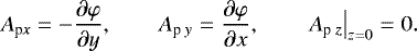
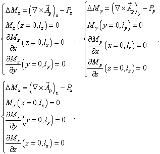
In order to solve for the vector potentials, the boundary conditions must be specified. First, we obtain the values of A p and A on all six boundaries (x = 0, lx;y = 0, ly;z = 0, lz). Taking the bottom boundary (z = 0) as an example, we define a new scalar function φ(x, y) that determines the vector potential Ap of potential magnetic field P corresponding to B on this boundary as follows:
 (3)
(3)
According to the definition of the vector potential, the scalar function φ(x, y) satisfies the Poisson equation:
 (4)
(4)
In our previous work (Yang et al. 2013) we set the values of ∂φ∕∂n at the four edges of the plane z = 0 to zero in Eq. (4). As a consequence, the corresponding magnetic flux at the boundary also vanish according to Ampère’s law. The values of Ap on the otherfive boundaries can be obtained in the same way. For the vector potential A at all boundaries, the same values are taken as for Ap. When the magnetic fluxes through the six boundaries are finite, we should calculate the values of vector potentials at the 12 edges of the 3D volume to obtain a Neumann boundary condition for the Poisson Eq. (4) at each side boundary. In the next section, we introduce a scheme to calculate the vector potentials at the 12 edges.
3 General method to obtain Ap and A at the boundaries
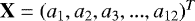
In order to determine Ap, we define the magnetic flux Φi (i = 1, …, 6) respectively at each side boundary (z = 0; z = lz; x = 0; x = lx; y = 0; y = ly). The integrals of ∫ Ap ⋅dl at the 12 edges are defined as ai (i = 1, …, 12). The 12 integrals and the corresponding directions are depicted in Fig. 1. Applying Ampère’s law to the six boundaries independently, we obtain a linear system of equations for obtaining the integral value ai
 (5)
(5)
where  ,
,  , and
, and  is a 6 × 12 matrix given by
![Mathematical equation: \begin{equation*} \tiny {\hat{\textbf{{T}}}}= \left[ \begin{array}{cccccccccccc} 1 & 1 & 1 & 1 & 0 & 0 & 0 & 0 & 0 & 0 & 0 & 0 \\ 0 & 0 & 0 & 0 & 1 & 1 & 1 & 1 & 0 & 0 & 0 & 0 \\ 0 & 0 & 0 &{-1}& 0 & 0 & 0 &{-1} & 1 & 0 & 0 & 1 \\ 0 &{-1} & 0 & 0 & 0 &{-1} & 0 & 0 & 0 & 1 & 1 & 0 \\ {-1}& 0 & 0 & 0 &{-1} & 0 & 0 & 0 &{-1} &{-1}& 0 & 0 \\ 0 & 0 &{-1}& 0 & 0 & 0 &{-1} & 0 & 0 & 0 &{-1}&{-1}\\ \end{array} \right].\end{equation*}](/articles/aa/full_html/2018/05/aa28108-16/aa28108-16-eq11.png) (6)
(6)
The six rows in this matrix are not linearly independent because the magnetic field is divergence-free and the sum of Φi through all six boundaries vanishes. Therefore, there are no unique solutions for the 12 integrals ai . We use the freedom in the gauge to construct 12 independent equations to obtain unique solutions for ai . We remove the last row of Eq. (6) and add another seven rows to define a new matrix  to make sure the determinant of
  is not zero without limiting the validity of the solution for ai. We choose the following seven rows to construct the new matrix
  :
:
![Mathematical equation: \begin{equation*} \tiny {\hat{\textbf{{T'}}}}= \left[ \begin{array}{ccccccccccccc} 1 & 1 & 1 & 1 & 0 & 0 & 0 & 0 & 0 & 0 & 0 & 0 \\ 0 & 0 & 0 & 0 & 1 & 1 & 1 & 1 & 0 & 0 & 0 & 0 \\ 0 & 0 & 0 &{-1}& 0 & 0 & 0 &{-1} & 1 & 0 & 0 & 1 \\ 0 &{-1} & 0 & 0 & 0 &{-1} & 0 & 0 & 0 & 1 & 1 & 0 \\ {-1}& 0 & 0 & 0 &{-1} & 0 & 0 & 0 &{-1} &{-1}& 0 & 0 \\ 1 & 0 &{-1}& 0 & 0 & 0 & 0 & 0 & 0 & 0 & 0 & 0 \\ 0 & 1 & 0 &{-1}& 0 & 0 & 0 & 0 & 0 & 0 & 0 & 0 \\ 0 & 0 & 1 & 0 & {-1}& 0 & 0 & 0 & 0 & 0 & 0 & 0 \\ 0 & 0 & 0 & 1 & 0 & {-1}& 0 & 0 & 0 & 0 & 0 & 0 \\ 0 & 0 & 0 & 0 & 1 & 0 & {-1}& 0 & 0 & 0 & 1 & 0 \\ 0 & 0 & 0 & 0 & 0 & 1 & 0 & {-1}& 0 & 0 & 0 & 0 \\ 0 & 0 & 0 & 0 & 0 & 0 & 1 & 0 & {-1}& 0 & 0 & 0 \\ \end{array} \right].\end{equation*}](/articles/aa/full_html/2018/05/aa28108-16/aa28108-16-eq15.png) (7)
(7)
This choice for the lower seven rows of  is not unique, but any influence on the gauge will be removed later. We can calculate that the determinant of
  does not vanish. According to Cramer’s rule, a unique solution of the new linear equation
 (8)
(8)
can exists if 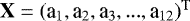 and
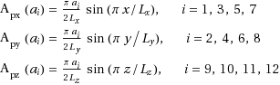
and  . Then we can obtain the integralsof ai at the 12 edges such that Gauss’s theorem applied to the Coulomb vector potentials in the volume V is satisfied. Since only the integral values ai are relevant in Eq. (3), the vector potentials at the 12 edges can be obtained representing the components of A p in the following way:
 (9)
(9)
It should be noted that such Ap by construction vanishes at the ends of every edge, i.e. at every corner of the box as required by Eq. (3). Now we solve the Poisson Eq. (4) to obtain Ap at the six boundaries. The vector potential A at the six boundaries is equal to A p . The following procedure corresponds to the Sects. 2.2 and 2.3 of Yang et al. (2013). Using the boundary conditions above, A p and A in the volume are obtained by solving the Poisson and Laplace equations
 (10)
(10)
everywhere in the volume if Ap satisfies the Coulomb gauge. The vector potential A of the original magnetic field B satisfies the Poisson equation
 (11)
(11)
where J = μ0j denotes the current density. In order to remove numerical errors and imperfections in the gauge, we implement a projection method that removes violations of the solenoidal constraint in the volume. In particular, we introduce a solenoidal modification vector ∇ × M satisfying the following condition:
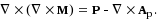 (12)
(12)
The components of M satisfy the three Poisson equations:
 (13)
(13)
Finally, in order to remove the residual errors in the solenoidal property of Ap, we introduce a scalar field ϕ(x, y, z) which satisfies the following Poisson equation:
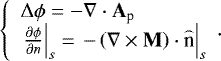 (14)
(14)
After solving Eq. (14), we obtain a new modified vector potential A′p, which is represented as
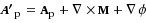 (15)
(15)
and in the same way, we can obtain the corrected vector potential A ′ just by replacing the right-hand side term of Eq. (13) as ∇×A −B. Now we can calculate the relative helicity in the volume according to Eq. (1). As already mentioned when introducing  , the choice of the lower seven rows of and the final seven elements of F′ is not unique.
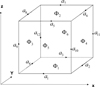 |
Fig. 1 Magnetic flux Φi (i = 1, …, 6) through the six boundaries and integration paths ai (i = 1, …, 12) along the 12edges of the volume. |
4 Testing the scheme
To test the new scheme for obtaining the vector potentials at the boundaries, we used the analytical non-linear force-free fields of Low & Lou (1990). We utilized the model labelled P1,1 with l = 0.3 and Φ = π∕2 in the notation of their paper. We calculated the magnetic field on a uniform grid of 64 × 64 × 64.
We first calculated the magnetic fluxes Φ0 through thesix boundaries and substituted it into Eq. (8) to obtain the integrals ai along the 12 edges of the 3D volume. Then we substituted ai into Eq. (9) to obtain the boundary value to solve the Poisson Eq. (4) at the six boundaries. After we obtained A p on the six boundaries, we calculated the magnetic fluxes Φ from the computed vector potential using the relation between the vector potential and the magnetic field:  . Table. 1 represents the quantitative result after applying the above scheme. As can be seen in the table, the magnetic fluxes through the six boundaries calculated via our new scheme is actually better flux-balanced than the theoretical model. Suchsmall errors are partly due to the fact that the total magnetic flux of the analytical model does not completely vanish. The total magnetic flux must be zero in order to resole the linear Eq. (8). Numerical errors in solving the Poisson equation, on the other hand, will also introduce finite total magnetic flux. The calculated relative magnetic helicity using the previous method is −14 441.45, while the value is −13 253.36 using the new method. There is an 8% difference for the two methods.
We then applied our new scheme to recalculate the relative magnetic helicity above active region NOAA AR8210 in Yang et al. (2013). Figure 2 depicts the comparison of relative magnetic helicity evolution by using the previous and the newscheme. The solid (dashed) line represents the new (previous) relative magnetic helicity evolution. The very small difference (<1.2%) is due to the magnetic field structure of the corona above AR8210 obtained by Yang et al. (2013) where the fluxes through the side boundaries were almost balanced.
Finally, we applied our new scheme to the 3D magnetic field data obtained from the simulated evolution of the solar corona above activeregion NOAA AR11429. The new GOEMHD3 code was used to reveal the magnetic field evolution in the solar atmosphere in response to the energy influx from the chromosphere through the transition region. The weak Joule current dissipation and a finite viscosity is taken into account in the almost dissipationless solar corona. The GOEMHD3 code is a massively parallel code for solving second-order accurate MHD equations (Skála et al. 2015). It was successfully tested and applied to study the magnetic coupling between the solar photosphere and corona based on multiwavelength observations. GOEMHD3 discretizes the ideal part of the MHD equations using a fast and efficient leap-frog scheme that is second-order accurate in space and time and whose initial and boundary conditions can easily be modified. For the investigation of diffusive and dissipative processes the corresponding terms are discretized by a DuFort-Frankel scheme. To always fulfil the Courant-Friedrichs-Lewy stability criterion, the time step of the code is adapted dynamically. Non-equidistant grids enhance the spatial resolution near the transition region. GOEMHD3 is parallelized based on a hybrid MPI-OpenMP programming paradigm, adopting a standard 2D domain-decomposition approach. This allows us to investigate the long time evolution of the relative magnetic helicity in the solar corona both in ideal and non-ideal magnetohydrodynamics by the non-ideal magnetohydrodynamical phase triggered by the switching on of resistivity.
Figure 3 shows the evolution of the relative magnetic helicity, using our method to simulate the data from the application of GOEMHD3, to the evolution of AR 11429 on March 07, 2012 (Skála et al. 2015). The vertical dash-dotted line in Fig. 3 indicates the time (t = 1035s) when fast reconnection started. Figure 3a depicts the evolution of relative magnetic helicity in the simulation box (solid line) and the accumulated relative helicity (dashed line) calculated using the helicity change rate Eq. (6) in the Yang et al. (2013). The surface integral in Eq. (6) of Yang et al. (2013) is extended to all six boundaries and the dissipative volume integral in Eq. (6) of Yang et al. (2013) is also included in the computation.
Figure 3b depicts the normalized magnetic helicity evolution (H∕Φ2). We used two types of fluxes Φ as the normalized parameter. One is unsigned magnetic flux only through the bottom boundary (solid line in Fig. 3b), which is usually used in observations. The other is unsigned magnetic flux through the six side boundaries (dashed line in Fig. 3b). A value of −0.038 (−0.025) was reachedafter fast reconnection started while choosing unsigned magnetic flux through the bottom boundary (side boundaries) as the normalized parameter. The calculated normalized value −0.039 (−0.026) is consistent with the above simulation results if we substitute the two types of fluxes into the formula between the magnetic helicity and themagnetic flux from the observations of newly emerging active regions (Yang et al. 2009b)
 (16)
(16)
where a = 1.85, b = −0.41, H0 = 1041Mx2, and Φ0 = 1021Mx., which describes the relation between the accumulated helicity ΔH and magnetic flux Φm for active regions. Figure 3c depicts the magnetic helicity flux through the bottom boundary into the solar corona. The total magnetic helicity flux is shown in Fig. 3d. We find that the negative magnetic helicity is injected into the Corona due to the subphotospheric plasma motion. The total injected helicity is − 8.5 × 1042Mx2. Figure 3e depicts the dissipation of magnetic helicity flux calculated as − 2 ∫ E ⋅ BdV . The helicity dissipation is enhanced due to fast magnetic reconnection, i.e. non-ideal magnetohydrodynamics. The integrated dissipated magnetic helicity flux is shown in Fig. 3f. We find that the sign of dissipation is positive, i.e. opposite to the helicity injected through the bottom boundary. The total magnetic helicity dissipation in the reconnection is 0.71 × 1042Mx2. We note that only 8% of the injected magnetic is dissipated. This reflects the fact that magnetic helicity is approximately conserved during fast magnetic reconnection as pointed out by (Taylor 1974). Figure 3g depicts the magnetic helicity flux which escapes through the upper five boundaries. The total escaped magnetic helicity evolution is shown in Fig. 3h. We find that only − 0.16 × 1042Mx2 of the magnetic helicity flux escapes through the upper boundaries. This is 23% of the dissipated helicity flux (0.71 × 1042Mx2, see Fig. 3f) and only 2% of the total injected magnetic helicity (− 8.5 × 1042Mx2, see Fig. 3d). We note that only the helicity flux through all six boundaries is gauge invariant, and that fluxes though individual boundaries have values that may change by changing gauge (Pariat et al. 2015). In the calculation of Fig. 3c-g at the separate boundary, we use the Coulomb gauge.
Results of the new scheme applied to the analytical model of Low & Lou (1990).
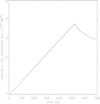 |
Fig. 2 Comparison of the magnetic helicity calculation by applying the previous and new schemes to the magnetic field data of Yang et al. (2013). The solid (dashed) line represents the new (previous) relative magnetic helicity evolution. |
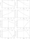 |
Fig. 3 Relative magnetic helicity evolution calculation using the result of the GOEMHD3 simulation. The dash-dotted line represents the time when the fast reconnection started (t = 1035s). (a) Relative magnetic helicity in the simulation box (dashedline) and the accumulated relative helicity (solid line) sum of the helicity injection through the boundary and the dissipated in the volume helicity according to Eq. (6) in Yang et al. (2013). (b) Evolution of the normalized relative helicity, where the magnetic helicity is normalized by unsigned flux at the bottom boundary (solid line) and the six side boundaries (dashed line). (c) Injected magnetic helicity flux through the bottom boundary. (d) Injected magnetic helicity from the bottom boundary. (e) Magnetic helicity dissipation rate in the simulation box. (f) Magnetic helicity dissipation in the simulation box. (g) Magnetic helicity change rate escaped from the other five boundaries except the bottom boundary. (h) Magnetic helicity escaped from the upper five boundaries. |
5 Summary and discussion
We propose a new generalized scheme to calculate the vector potential at the boundaries of a closed volume without the restrictions of the method applied in the previous paper (Yang et al. 2013). We verified the new method using an analytical theoretical force-free model magnetic field (Low & Lou 1990) and the simulated data in Yang et al. (2013). We also applied the new methodto simulated coronal magnetic fields using the newly developed GOEMHD3 to investigate the magnetic helicity evolution of solar corona in the course of the evolution of AR11429.
We find that only 8% of the accumulated injected magnetic helicity is dissipated. This is consistent with the Taylor conjecture and also with the recent simulation results of Pariat et al. (2015). Only 2% of the magnetic helicity injected through the bottom boundary escapes to the solar wind. This shows that the magnetic helicity cannot efficiently escape. This may help us to understand the lack of magnetic clouds1 with considerable magnetic helicity in the interplanetary space (Janvier et al. 2015). This is true even though several halo CMEs originated from the simulated active region AR11492.
Our simulation results further confirm that the absolute normalized magnetic helicity (H∕Φ2) reaches 0.038 after the reconnection starts. It is interesting to note that recently an isolated and quickly decaying active region (NOAA 9729) was studied in detail as it passed across the solar disk. There was only one CME associated with that active region. This provided a good opportunity to investigate the consequences of a single CME after the injection of magnetic helicity to the solar corona. The absolute value of normalized magnetic helicity was 0.036 just after solar eruption happened (Yang et al. 2015). This is also similar to the obtained simulation results. A normalized helicity is one order of magnitude smaller than the value −0.16 (−0.18) obtained by the MHD simulation results of kink or torus instability of ideal MHD (Fan & Gibson 2007) when eruption happened. This might be due to the anomalous resistivity caused by the strong micro-turbulence and microscopic structures (Büchner & Elkina 2006) used in the GOEMHD3 model. The anomalous current dissipations allows the dissipation rate of magnetic energy to essentially increase following a global MHD instability (Büechner et al., in preparation).
Zhang et al. (2006) and Zhang & Flyer (2008) proposed that there is an upper bound of the total magnetic helicity that a force-free field can contain in a multipolar force-free magnetic field structure before eruption, which is very close to the value obtained above. However, the allowable level of helicity in a force-free field is only a sufficient condition for an eruption. A CME expulsion may still occur even before this helicity limit is reached (Zhang et al. 2006). The upper-bound normalized magnetic helicity value clearly deviates for different magnetic structures in the theoretical force-free field model. For multipolar fields, the helicity upper bound can be 10 times smaller than that of a dipolar field (Zhang & Flyer 2008), but in our observations and simulation result, the normalized helicity reaches the same order when eruption happens. It is essential to investigate the evolution of magnetic helicity and energy using more observations and simulations in future studies.
Above all, after introducing a new scheme removing the former restriction on the magnetic flux through the boundaries, we can calculate the relative magnetic helicity of any magnetic field structure in Cartesian coordinates. In the observations, we could use a force-free extrapolation to obtain the 3D magnetic structure to analyse the evolution of relative magnetic helicity.
Acknowledgements
We would like to thank the referee for carefully reading our manuscript and for giving such constructive comments which substantially helped to improve the paper. This study is supported by grants 11427901, 10921303, 11673033, U1731113,11611530679, and 11573037 of the National Natural Science Foundation of China; by grant No. XDB09040200, XDA15010700 of the Strategic Priority Research Program of Chinese Academy of Sciences; by the Max-Planck Society Interinstitutional Research Initiative Turbulent transport and ion heating, reconnection, and electron acceleration in solar and fusion plasmas of Project No. MIF-IF-A-AERO8047; by Max-Planck-Princeton Center for Plasma Physics PS AERO 8003; by ISSI International Team on Magnetic Helicity estimations in models and observations of the solar magnetic field. The authors would also like to thank the Supercomputing Center of the Chinese Academy of Sciences (SCCAS) and the Max-Planck Computing and Data Facility (MPCDF) for the allocation of computing time.
References
- Amari, T., Luciani, J. F., Aly, J. J., Mikic, Z., & Linker, J. 2003, ApJ, 585, 1073 [NASA ADS] [CrossRef] [Google Scholar]
- Berger, M. A. 1999, Plasma Phys. Contr. Fusion, 41, 167 [Google Scholar]
- Berger, M. A., & Field, G. B. 1984, J. Fluid Mech., 147, 133 [NASA ADS] [CrossRef] [Google Scholar]
- Büchner, J., & Elkina, N. 2006, Phys. Plasmas, 13, 082304 [NASA ADS] [CrossRef] [Google Scholar]
- Cane, H. V., & Richardson, I. G. 2003, J. Geophys. Res., 108, A4 [Google Scholar]
- Chae, J. 2001, ApJ, 560, L95 [NASA ADS] [CrossRef] [Google Scholar]
- Démoulin, P., & Berger, M. A. 2003, Sol. Phys., 215, 203 [CrossRef] [Google Scholar]
- Démoulin, P., & Pariat, E. 2009, Adv. Space Res., 43, 1013 [CrossRef] [Google Scholar]
- Fan, Y., & Gibson, S. E. 2007, ApJ, 668, 1232 [Google Scholar]
- Jacobs, C., Poedts, S., & van der Holst, B. 2006, A&A, 450, 793 [NASA ADS] [CrossRef] [EDP Sciences] [Google Scholar]
- Janvier, M., Dasso, S., Démoulin, P., Masías-Meza, J. J., & Lugaz, N. 2015, J. Geophys. Res., 120, 3328 [CrossRef] [Google Scholar]
- LaBonte, B. J., Georgoulis, M. K., & Rust, D. M. 2007, ApJ, 671, 955 [CrossRef] [Google Scholar]
- Low, B. C., & Lou, Y.Q. 1990, ApJ, 352, 343 [NASA ADS] [CrossRef] [Google Scholar]
- Liu, Y., Hoeksema, J. T., Bobra, M., et al. 2014, ApJ, 785, 13 [NASA ADS] [CrossRef] [Google Scholar]
- Nindos, A., & Andrews, M. D. 2005, Proc. IAU Symp., 226, 194 [NASA ADS] [Google Scholar]
- Pariat, E., Démoulin, P., & Berger, M. A. 2005, A&A, 439, 1191 [NASA ADS] [CrossRef] [EDP Sciences] [Google Scholar]
- Pariat, E., Valori, G., Démoulin, P., & Dalmasse, K. 2015, A&A, 580, A128 [NASA ADS] [CrossRef] [EDP Sciences] [Google Scholar]
- Park, S.-H., Lee, J., Choe, G. S., et al. 2008, ApJ, 686, 1397 [NASA ADS] [CrossRef] [Google Scholar]
- Pipin, V. V., & Pevtsov, A. A. 2014, ApJ, 789, 21 [Google Scholar]
- Richardson, I. G., & Cane, H. V., 2010, Sol. Phys., 264, 189 [NASA ADS] [CrossRef] [Google Scholar]
- Rudenko, G. V., & Myshyakov, I. I. 2011, Sol. Phys., 270, 165 [NASA ADS] [CrossRef] [Google Scholar]
- Santos, J. C., Büchner, J., & Otto, A. 2011, A&A, 535, A111 [NASA ADS] [CrossRef] [EDP Sciences] [Google Scholar]
- Schuck, P. W. 2008, ApJ, 683, 1134 [NASA ADS] [CrossRef] [Google Scholar]
- Seehafer, N., Gellert, M., Kuzanyan, K. M., & Pipin, V. V. 2003, AdSpR, 32, 1819 [NASA ADS] [CrossRef] [Google Scholar]
- Skála, J., Baruffa, F., Büchner, J., & Rampp, M. 2015, A&A, 580, A48 [NASA ADS] [CrossRef] [EDP Sciences] [Google Scholar]
- Taylor, J. B. 1974, Phys. Rev. Lett., 33, 1139 [NASA ADS] [CrossRef] [Google Scholar]
- Thalmann, J. K., Inhester, B., & Wiegelmann, T. 2011, Sol. Phys., 272, 243 [NASA ADS] [CrossRef] [Google Scholar]
- Tian, L., & Alexander, D. 2008, ApJ, 673, 532 [NASA ADS] [CrossRef] [Google Scholar]
- Tziotziou, K., Georgoulis, M. K., & Raouafi, N.-E. 2012, ApJ, 759, L4 [NASA ADS] [CrossRef] [Google Scholar]
- Valori, G., Démoulin, P., & Pariat, E. 2012, Sol. Phys., 278, 347 [NASA ADS] [CrossRef] [EDP Sciences] [Google Scholar]
- Valori, G., Pariat, E., Anfinogentov, S., et al. 2016, Space Sci. Rev., 201, 147 [NASA ADS] [CrossRef] [Google Scholar]
- Woltjer, L. 1958, Proc. Natl Acad. Sci. USA, 44, 480 [NASA ADS] [Google Scholar]
- Yang, S., Büchner, J., & Zhang, H. 2009a, ApJ, 695, L25 [Google Scholar]
- Yang, S., Zhang, H., & Büchner, J. 2009b, A&A, 502, 333 [NASA ADS] [CrossRef] [EDP Sciences] [Google Scholar]
- Yang, S., Büchner, J., Santos, J. C., & Zhang, H. 2013, Sol. Phys., 283, 369 [NASA ADS] [CrossRef] [Google Scholar]
- Yang, S., Xie, W., & Liu, J. 2015, AdSpR, 55, 1553 [NASA ADS] [Google Scholar]
- Zhang, M., & Flyer, N. 2008, ApJ, 683, 1160 [NASA ADS] [CrossRef] [Google Scholar]
- Zhang, M., Flyer, M., & Low, B. 2006, ApJ, 644, 575 [NASA ADS] [CrossRef] [Google Scholar]
- Zhang, Y., Tan, B. L., & Yan, Y. H. 2008, ApJ, 682, L133 [NASA ADS] [CrossRef] [Google Scholar]
Near-Earth Interplanetary Coronal Mass Ejections Since January 1996: www.srl.caltech.edu/ACE/ASC/DATA/level3/icmetable2.htm. It is described in Cane & Richardson (2003); Richardson & Cane (2010).
All Tables
All Figures
|
Fig. 1 Magnetic flux Φi (i = 1, …, 6) through the six boundaries and integration paths ai (i = 1, …, 12) along the 12edges of the volume. |
| In the text | |
|
Fig. 2 Comparison of the magnetic helicity calculation by applying the previous and new schemes to the magnetic field data of Yang et al. (2013). The solid (dashed) line represents the new (previous) relative magnetic helicity evolution. |
| In the text | |
|
Fig. 3 Relative magnetic helicity evolution calculation using the result of the GOEMHD3 simulation. The dash-dotted line represents the time when the fast reconnection started (t = 1035s). (a) Relative magnetic helicity in the simulation box (dashedline) and the accumulated relative helicity (solid line) sum of the helicity injection through the boundary and the dissipated in the volume helicity according to Eq. (6) in Yang et al. (2013). (b) Evolution of the normalized relative helicity, where the magnetic helicity is normalized by unsigned flux at the bottom boundary (solid line) and the six side boundaries (dashed line). (c) Injected magnetic helicity flux through the bottom boundary. (d) Injected magnetic helicity from the bottom boundary. (e) Magnetic helicity dissipation rate in the simulation box. (f) Magnetic helicity dissipation in the simulation box. (g) Magnetic helicity change rate escaped from the other five boundaries except the bottom boundary. (h) Magnetic helicity escaped from the upper five boundaries. |
| In the text | |
Current usage metrics show cumulative count of Article Views (full-text article views including HTML views, PDF and ePub downloads, according to the available data) and Abstracts Views on Vision4Press platform.
Data correspond to usage on the plateform after 2015. The current usage metrics is available 48-96 hours after online publication and is updated daily on week days.
Initial download of the metrics may take a while.