| Issue |
A&A
Volume 612, April 2018
|
|
|---|---|---|
| Article Number | A95 | |
| Number of page(s) | 11 | |
| Section | Planets and planetary systems | |
| DOI | https://doi.org/10.1051/0004-6361/201732217 | |
| Published online | 04 May 2018 | |
K2-141 b
A 5-M⊕ super-Earth transiting a K7 V star every 6.7 h★,★★
1
Dipartimento di Fisica, Università degli Studi di Torino,
via Pietro Giuria 1,
10125
Torino, Italy
e-mail: This email address is being protected from spambots. You need JavaScript enabled to view it.
2
Department of Physics and Kavli Institute for Astrophysics and Space Research, Massachusetts Institute of Technology,
Cambridge,
MA
02139, USA
3
Department of Astrophysical Sciences, Princeton University,
4 Ivy Lane,
Princeton,
NJ
08544, USA
4
Department of Astronomy, Graduate School of Science, The University of Tokyo,
Hongo 7-3-1,
Bunkyo-ku,
Tokyo
113-0033, Japan
5
Department of Space, Earth and Environment, Chalmers University of Technology, Onsala Space Observatory,
439 92 Onsala, Sweden
6
Department of Earth and Planetary Sciences, Tokyo Institute of Technology,
2-12-1 Ookayama,
Meguro-ku,
Tokyo
152-8551, Japan
7
Astrobiology Center, NINS,
2-21-1 Osawa,
Mitaka,
Tokyo
181-8588, Japan
8
National Astronomical Observatory of Japan, NINS,
2-21-1 Osawa,
Mitaka,
Tokyo
181-8588, Japan
9
Institute of Planetary Research, German Aerospace Center,
Rutherfordstrasse 2,
12489
Berlin, Germany
10
Departamento de Astrofísica, Universidad de La Laguna,
38206
Tenerife, Spain
11
Instituto de Astrofísica de Canarias,
C/ Vía Láctea s/n,
38205
La Laguna,
Tenerife, Spain
12
Stellar Astrophysics Centre, Department of Physics and Astronomy, Aarhus University,
Ny Munkegrade 120,
8000
Aarhus C, Denmark
13
Department of Astronomy and McDonald Observatory, University of Texas at Austin,
2515 Speedway, Stop C1400,
Austin,
TX
78712, USA
14
Leiden Observatory, University of Leiden,
PO Box 9513,
2300
RA
Leiden, The Netherlands
15
Okayama Astrophysical Observatory, National Astronomical Observatory of Japan,
Asakuchi,
Okayama
719-0232, Japan
16
Rheinisches Institut für Umweltforschung, Abteilung Planetenforschung an der Universität zu Köln,
Aachener Strasse 209,
50931
Köln, Germany
17
Thüringer Landessternwarte Tautenburg,
Sternwarte 5,
07778
Tautenberg, Germany
18
Department of Astronomy, The Ohio State University,
140 West 18th Ave.,
Columbus,
OH
43210, USA
19
Center for Astronomy and Astrophysics, TU Berlin,
Hardenbergstr. 36,
10623
Berlin, Germany
Received:
31
October
2017
Accepted:
11
January
2018
Abstract
We report on the discovery of K2-141 b (EPIC 246393474 b), an ultra-short-period super-Earth on a 6.7 h orbit transiting an active K7 V star based on data from K2 campaign 12. We confirmed the planet’s existence and measured its mass with a series of follow-up observations: seeing-limited MuSCAT imaging, NESSI high-resolution speckle observations, and FIES and HARPS high-precision radial-velocity monitoring. K2-141 b has a mass of 5.31 ± 0.46 M⊕ and radius of 1.54−0.09+0.10 R⊕, yielding a mean density of 8.00−1.45+1.83 g cm−3 and suggesting a rocky-iron composition. Models indicate that iron cannot exceed ~70% of the total mass. With an orbital period of only 6.7 h, K2-141 b is the shortest-period planet known to date with a precisely determined mass.
Key words: planetary systems / planets and satellites: individual: EPIC 246393474 b / stars: fundamental parameters / stars: individual: EPIC 246393474 / techniques: photometric / techniques: radial velocities
Based on observations obtained with (a) the Nordic Optical Telescope (NOT), operated on the island of La Palma jointly by Denmark, Finland, Iceland, Norway, and Sweden, in the Spanish Observatorio del Roque de los Muchachos (ORM) of the Instituto de Astrofisica de Canarias (IAC); (b) the 3.6m ESO telescope at La Silla Observatory under program ID 099.C-0491; (c) the Kepler space telescope in its extended mission K2.
Tables of the light curve data and the radial velocities are only available at the CDS via anonymous ftp to cdsarc.u-strasbg.fr (130.79.128.5) or via http://cdsarc.u-strasbg.fr/viz-bin/qcat?J/A+A/612/A95
© ESO 2018
1 Introduction
Short-period (Porb ≲ 10 days) exoplanets are interesting and convenient targets for radial velocity (RV) follow-up observations. The shorter the period, the larger the amplitude of the Doppler reflex motion induced by the planet on its host star, and the easier it is to sample the orbital motion in an observing campaign. This helps to explain why the ultra-short-period (USP; P < 1 day) planets have often been the targets of recent RV programs. With periods shorter than 1 day, and sizes almost always smaller than 2 R⊕, transiting USP planets offer relatively easy access to knowledge of the properties of terrestrial-sized objects (Sanchis-Ojeda et al. 2014). The radius domain of USP planets includes the gap between 1.5 and 2 R⊕ in the bimodal distribution found in the Kepler sample by Fulton et al. (2017). Van Eylen et al. (2017) found a similar result using a small sample with stellar parameters coming from asteroseismology measurements, which includes transiting planets with radius determinations of ~ 3%. This gap has been predicted by photo-evaporation models (e.g., Lopez & Fortney 2014; Owen & Wu 2013), in which close-in planets can lose their entire atmospheres due to stellar irradiation. In this context, USP planets are expected to be atmosphere-free, bare, solid planets. Accurate mass measurements of transiting USP planets will be helpful to test this theory. They may also help to determine whether there is substantial variation in the balance of rock and iron in terrestrial planets (e.g., Pepe et al. 2013; Gandolfi et al. 2017; Guenther et al. 2017).
Sanchis-Ojeda et al. (2014) suggested that USP planets are the remnant cores of hot Jupiters that lost their gaseous envelopes due to photo-evaporation. However, Winn et al. (2017) found that the strong tendency for gas-giant planets to be found around metal-rich stars does not hold for USP planets, contrary to what one would expect if hot Jupiters are the progenitors of USP planets. This leaves open the possibility that hot Neptunes are the progenitors of USP planets, because the occurrence rate of planets smaller than 4 R⊕ does not appear to be strongly dependent on the host star metallicity (Buchhave et al. 2012; Buchhave & Latham 2015). Accurate determinations of masses and radii of USP planets – with uncertainties of 20% or smaller – along with spectral analyses of the host stars would enable searches for possible correlations between stellar composition and the properties of USP planets (e.g., Dumusque et al. 2014b; Gandolfi et al. 2017).
In this paper we present the discovery of K2-141 b (EPIC 246393474 b), an USP planet transiting a K7 V star. The use of state-of-the-art spectrographs and an optimal observing strategy allowed us to pin down the planetary mass with an uncertainty better than 10%. These results are part of the ongoing project carried out by the KESPRINT consortium to detect, confirm, and characterize transiting planets from the K2 mission (e.g., Barragán et al. 2016, 2018; Dai et al. 2017; Fridlund et al. 2017; Johnson et al. 2016; Narita et al. 2017; Nespral et al. 2017; Sanchis-Ojeda et al. 2015; Smith et al. 2017).
2 K2 photometry
K2’s campaign 12 (C12) was carried out by the Kepler space telescope from December 15, 2016, to March 4, 2017, UTC. The spacecraft was pointed towards the coordinates αJ2000 = 23h26m38s, δJ 2000 = −05°06′08″. The photometric data include 79 days of almost continuous observations with a gap of 5.3 days between February 01, 15:06 UTC and February 06, 20:47 UTC when the satellite entered a safe mode. The C12 target list included 29 221 targets monitored in long-cadence mode, and 141 in short-cadence mode3. We downloaded the calibrated target pixel files from the Mikulski Archive for Space Telescopes4 and extracted the light curves using an approach similar to that described by Vanderburg & Johnson (2014). For each image, we laid down a 16″ -wide circular aperture around the brightest pixel, and fitted a two-dimensional (2D) Gaussian function to the intensity distribution. We then fitted apiecewise linear function between the observed flux variation and the best-fitting central coordinates of the Gaussian function.
Before searching the light curves for transits, we attempted to remove long-term systematic or instrumental flux variations by normalizing the light curve using 1.5-day-long cubic splines. We searched for periodic transit signals using the Box-Least-Squares algorithm (BLS; Kovács et al. 2002) and employed a nonlinear frequency grid to account for the expected scaling of transit duration with orbital period. We also adopted Ofir (2014)’s definition of signal detection efficiency (SDE). We discovered that the light curve of EPIC 246393474 (hereafter K2-141) – whose equatorial coordinates, proper motion, parallax, and optical and near-infrared magnitudes are listed in Table 1 – shows periodic transit-like signal with a SDE of 23.5 and a depth of ~0.04% occurring every 0.28 days (6.7 h). We searched for additional transiting planets in the system by re-running the BLS algorithm after removing the data within 1.5 h of each transit of planet b. No transit signal was detected: the maximum SDE of the new BLS spectrum was 4.5. A visual inspection of the light curve did not reveal any additional transits, either. The target passed standard tests used to detect false positives due to eclipsing binaries: we did not detect any secondary eclipses or alternation of eclipse depths.
The K2 light curve of K2-141 shows quasi-periodic variations with a peak-to-peak amplitude of about ~1%, very likely the result of rotation and active regions on the host star (Fig. 1). This is further discussed in Sect. 5. Using the auto-correlation method applied to the out-of-transit K2 light curve (McQuillan et al. 2014), we measured a stellar rotation period of Prot = 14.03 ± 0.09 days.
Main identifiers, coordinates, optical and infrared magnitudes, and proper motion of K2-141.
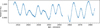 |
Fig. 1 K2 light curve of K2-141. Stellar activity is seen as the quasi-periodic, long period modulation. Transits are visible as shallow dips. The 5.3-day-long data gap, during which the telescope entered safe mode, is clearly visible at approximately two-thirds of the way through the time series. |
3 Ground-based follow-up observations
Kepler’s charge-coupled device (CCD) have a sky-projected pixel size of ~4″. Ground-based imaging with higher angular resolution is useful to check for an unresolved eclipsing binary that might be the source of the transit signal. Imaging is also useful to measure the fraction of light in the K2 photometric aperture that originates from the target star as opposed to other nearby stars. This is important for establishing the true fractional variation in the starlight during transits, and thereby the planet radius. Finally, high-precision RV measurements are needed to confirm the planetary nature of the transiting object and to measure its mass.
3.1 Diffraction-limited imaging
On the night of August 9, 2017, UT, we conducted speckle imaging observations of the star K2-141 with the NASA Exoplanet Star and Speckle Imager (NESSI; Scott et al., in prep.), a new instrument for the WIYN 3.5 m telescope, which uses high-speed electron-multiplying CCDs (EMCCDs) to capture sequences of 40 ms exposures simultaneously in two bands. We also observed nearby point source calibrator stars close in time to the science target. We observed simultaneously in the “blue” band centered at 562 nm with a width of 44 nm and the “red” band centered at 832 nm with a width of 40 nm. The pixel scales of the “blue” and “red” EMCCDs are 0.0175649 and 0.0181887″ pixel−1, respectively. The data reduction followed the same procedures described by Howell et al. (2011). Using the point source calibrator images, we computed reconstructed 256 × 256 pixel images in each band, corresponding to 4.6″ × 4.6″. Figure 2 shows the contrast curves and reconstructed images for the “blue” and “red” pass bands. No secondary sources were detected in the reconstructed images. We measured the background sensitivity of the reconstructed images using a series of concentric annuli centered on the target star, resulting in 5σ sensitivity limits (in delta-magnitudes) as a function of angular separation.
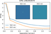 |
Fig. 2 “Blue” and “red” contrast curves and reconstructed images of K2-141 (insets). The two images are both centered around K2-141 and have a size of 4.6″× 4.6″. |
3.2 Seeing-limited imaging
In order tosearch for sources outside of the 4.6″ × 4.6″ field-of-viewof our high-resolution NESSI images, but within the 16″ -wide circular aperture used to extract the light curve from the K2 pixel files, we also obtained seeing-limited multi-band optical images using the MuSCAT (Narita et al. 2015) instrument on the 1.88 m telescope at the Okayama Astrophysical Observatory. The pixel scale of MuSCAT’s CCDs is 0.36″ pixel−1. The instrument can observe in Sloan  ,
,  , and zs,2 bands simultaneously. The observations were performed on September 23, 2017 UT with seeing of ~1.5″. To keep thepeak count level at about 45 000 ADU, we took ten exposures of 15, 4, and 12 s with the
  ,
,  , and zs,2 bands, respectively. The frames were dark-subtracted and flat-fielded using standard routines. The five best on-focus frames were stacked together for each band.
We detected a companion located at 12.6″ towards the East of K2-141. MuSCAT’s images show that this target is about 7.8 mag fainter than K2-141 (from the weighted averaged of the  and
and  filters). This accounts for a contamination factor of 1∕1400 of the target brightness. This value does not have a measurable impact on the derived parameters.
3.3 High-precision Doppler observations
We started the RV follow-up of K2-141 with the FIbre-fed Échelle Spectrograph (FIES; Frandsen & Lindberg 1999; Telting et al. 2014) mounted at the 2.56 m Nordic Optical Telescope (NOT) of Roque de los Muchachos Observatory (La Palma, Spain). We obtained nine high-resolution (R ≈ 67 000) spectra on five different nights, from August 15 to September 14, 2017, UTC, within observing programs 55-019, 55-202, and 55-206. Since the 6.7-h period is short enough to allow a significant fraction of the orbit to be sampled in one night, we obtained two spectra per night during three of the five FIES observing nights. Following (Gandolfi et al. 2015), we traced the RV drift of the instrument by bracketing the science exposures with 90-s ThAr spectra. We reduced the data using standard IRAF and IDL routines and extracted the RVs via multi-order cross-correlations using the stellar spectrum with the highest signal-to-noise ratio (S/N) as a template.
We also acquired 27 spectra with the HARPS spectrograph (R ≈ 115 000; Mayor et al. 2003) mounted at the ESO-3.6 m telescope of La Silla observatory (Chile), as part of the observing program 099.C-0491. We adopted the same observing strategy as the FIES observations, acquiring between two and five spectra per night on seven different nights, from August 19 to 27, 2017, UTC. We reduced the data using the dedicated off-line HARPS pipeline and extracted the RVs via cross-correlation with a K5 numerical mask. The pipeline provides also the bisector span (BIS) and full-width at half maximum (FWHM) of the cross-correlation function, along with the Mt. Wilson activity index S of the Ca II H & K lines. Table 4 reports the FIES and HARPS RV measurements, as well as the exposure times and S/N per pixel at 5500 Å.
4 Stellar fundamental parameters
We derived the spectroscopic parameters of K2-141 from the co-added HARPS spectrum, which has a S/N per pixel of ~250. We used Spectroscopy Made Easy (SME; Valenti & Piskunov 1996; Valenti & Fischer 2005; Piskunov & Valenti 2017), a spectral analysis package that calculates synthetic spectra and fits them to high-resolution observed spectra using a χ2 minimizing procedure. The analysis was performed with the non-LTE SME version 5.2.2, along with ATLAS12 model atmospheres (Kurucz 2013). The microturbulent and macroturbulent velocities were assumed to be 1 km s−1 (Gray 2008). The wings of the Hα and Hβ lines were used to measure the effective temperature Teff. We excluded the core of the Balmer line because of their origin in higher layers of stellar photospheres. The surface gravity log g⋆ was determined from the wings of the Ca I λ 6102, λ 6122, λ 6162 Å triplet, and the Ca I λ 6439 Å line. We measured the iron abundance [Fe/H] and projected rotational velocity v sin i⋆ by simultaneously fitting many unblended iron lines in the spectral region 5880–6600 Å.
An independent analysis was carried out with SpecMatch-emp (Yee et al. 2017), a tool that uses hundreds of Keck/HIRES high-resolution template spectra of FGK stars for which the parameters have been accurately measured via interferometry, asteroseismology, spectral synthesis, and spectrophotometry. SpecMatch-emp finds the templates that best match an input observed spectrum in the spectral region 5000–5900 Å and derives the effective temperature Teff, stellar radius R⋆, and iron abundance [Fe/H] by interpolation.
We summarize the results of the two spectral analyses in Table 2. The effective temperature and iron abundance estimates are consistent well within the nominal error bars. Since the two methods are based on different wavelength regions (λ > 5880 Å for SME and λ < 5900 Å for SpecMatch-emp) we treated the two sets of parameters as independent estimates. For Teff and [Fe/H], we computed the weighted means of the values derived from the two methods. For the projected rotational velocity v sin i⋆ we adopted thevalue determined with SME. We report the adopted effective temperature Teff, iron abundance [Fe/H], and projected velocity v sin i⋆ in Table 3. The stellar radius and surface gravity were re-determined using a different method, as described in the next paragraphs.
We derived the stellar radius R⋆ and reddening Av following the method described in Gandolfi et al. (2008). Briefly, we first built the spectral energy distribution (SED; Fig. 3) of K2-141 from the optical and infrared photometry listed in Table 1. We then fitted the SED using the BT-Settl-CIFIST (Baraffe et al. 2015) model spectrum with the same spectroscopic parameters as the star. Adopting the extinction law of Cardelli et al. (1989) and assuming a total-to-selective extinction of R = Av∕EB−V = 3.1, we found that the interstellar reddening is consistent with zero (Av = 0.01 ± 0.02 mag). Using the distance of d = 58.77 ± 0.81 pc from the Gaia’s first data release (Table 1; Gaia Collaboration 2016), we determined a stellar radius of R⋆ = 0.674 ± 0.039R⊙, in agreement with the spectroscopic value derived using SpecMatch-emp (see Table 2).
An independent fit of the SED performed with the VOSA SED fitting tool (Bayo et al. 2008) yielded a stellar radius of R⋆ = 0.671 ± 0.042R⊙. We also verified our results combining the Gaia distance, effective temperature, and V J magnitude (Table 1) with the bolometric correction calculated from the empirical equations by Torres (2010) and found a radius of R⋆ = 0.666 ± 0.065R⊙. Both values are in excellent agreement with our measurement, adding confidence to our results.
We finally converted Teff, R⋆, and [Fe/H] into stellar mass M⋆ and surface gravity log g⋆ using the empirical relations derived by Torres et al. (2010) coupled to Monte Carlo simulations. K2-141 is a K7 V star (Pecaut & Mamajek 2013) with an effective temperature of Teff = 4373 ± 57 K, a photospheric iron abundance of [Fe/H] = + 0.03 ± 0.10 dex, a mass of M⋆ = 0.662 ± 0.022M⊙, and a radius of R⋆ = 0.674 ± 0.039R⊙, yielding a surface gravity of log g⋆ = 4.584 ± 0.051 (cgs). The final adopted values are given in Table 3. We note that also log g⋆ is consistent with our spectroscopic surface gravity (Table 2).
We used gyrochronology to estimate the age of K2-141 from the relations by Angus et al. (2015) and found 740 ± 360 Myr, suggesting that the star might be relatively young (Table 3).
Stellar and planetary parameters.
FIES and HARPS measurements of K2-141.
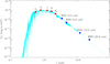 |
Fig. 3 Spectral energy distribution of K2-141. The BT-Settl-CIFIST model spectrum with the same parameters as the star is plotted with a light blue line. The V J, IC, J, H, Ks, W1, W2, W3, and W4 fluxes are derived from the magnitudes reported in Table 1. |
5 Stellar activity and frequency analysis of the HARPS data
K2-141 is an active star. As presented in Sect. 2, the K2 light curve of K2-141 displays quasi-periodic modulation with a peak-to-peak amplitude of about 1% (Fig. 1). The photometric variability is very likely caused by active regions (spots, faculae, and plages) carried across the visible hemisphere of the stellar disk as the star spins about its axis. This is corroborated by the detection of strong emission components in the cores of the Ca II H & K lines (Fig. 4), from which we derived an average S-index of 0.938 ± 0.074, indicative ofa high level of magnetic activity.
The magnetic activity of K2-141 is expected to produce quasi-periodic signals in time-series RV data, commonly referred to as “stellar jitter”. We used the code SOAP2 (Dumusque et al. 2014a) to estimate the RV variation induced by stellar activity. From the amplitude of the photometric variability, the spectroscopic parameters, and the rotation period of the star, we calculated an expected RV semi-amplitude variation of ~5–10 m s−1.
We performed a frequency analysis of our RV measurements to look for the signature of the transiting planet and search for possible activity-induced signals. For this purpose, we did not include the FIES RVs because of the higher uncertainties, the relatively small number of data points, and the need to account for an offset between the FIES and HARPS data-sets.
Figure 5 shows the discrete Fourier transform (DFT) of the 27 HARPS RV measurements calculated using the code Period04 (Lenz & Breger 2004). The peak with the largest semi-amplitude (~7 m s−1) is found to be at 3.57 c/d, that is, the orbital frequency of K2-141 b (0.28 day). We note that the semi-amplitude agrees with the value derived in Sect. 6. We also note the presence in the DFT of the 1-, 2-, 3-, and 4-day aliases to the left and right of the planetary signal, as expected given the 1-day sampling of our observations.
An additional trend is visible in the RV data after the signal of the transiting planet has been subtracted from the HARPS measurements, as depicted in the upper panel of Fig. 6. We found a Spearman’s rank correlation coefficient of − 0.80 with a p-value of 1.4 × 10⁻⁶, strongly suggesting the existence of an additional source of RV variation in our data5. To assess if the source of this additional signal is induced by stellar activity, we looked for possible correlations between the RV residuals and the activity indexes, namely, the Ca II H & K S-index, and the FWHM and bisector span (BIS) of the cross-correlation function (Fig. 6). Although the RV residuals and the BIS do not show a significant anti-correlation (− 0.30 with p = 0.13), we found significant correlations between the RV residuals and the FWHM (0.73 with p = 3.3 × 10⁻⁵), and the RV residuals and the S-index (0.72 with p = 4.8 × 10⁻⁵). We concluded that the long-term trend observed in the HARPS data is likely caused by the presence of active regions on the photosphereof the star. We will present our approach to filtering out the stellar jitter in the following section.
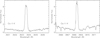 |
Fig. 4 Cores of the Ca II H & K lines of K2-141 as observed with HARPS. |
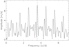 |
Fig. 5 Discrete Fourier transform of the HARPS RV measurements. The dashed red line marks the frequency at the orbital period of K2-141 b. |
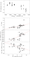 |
Fig. 6 Upper panel: HARPS RV residuals following the subtraction of the transiting planet signal vs. time. Lower panels: Ca II H&K S activity index (top), cross-correlation FWHM (middle), and cross-correlation bisector span (bottom) vs. RV residuals. The dashed red lines mark the best fitting linear fit. |
6 Data analysis and results
In order to arrive at a robust measurement of the planetary mass despite the additional RV variations induced by stellar activity (see Sect. 5), we used three different approaches to fit the data as described below.
6.1 Floating chunk offset method
The first method (hereafter M1) is based on the floating chunk offset (FCO) technique pioneered by Hatzes et al. (2011), which works well when the orbital period is much shorter than the timescales associated with the signals induced by stellar activity andany additional planets. The FCO method divides a given RV time-series into sub-segments of duration t, usually long enough to encompass the RV data collected within a given night. For each sub-segment, an offset is fitted to account for RV signals whose time-scales ≫ t, assuming that the offset remains constant within one night. From this point of view, K2-141 b is an ideal target to apply the FCO method and remove long-term signals coming from outer companions and stellar activity (see, e.g., Hatzes et al. 2011; Gandolfi et al. 2017). Our observing strategy was tailored to use this technique by acquiring multiple spectra per night (Sect. 3.3).
We performed a Markov chain Monte Carlo (MCMC) joint analysis of the transit and RV data using the code pyaneti (Barragán et al. 2017). We fitted a Keplerian orbit to the RV data and used the limb-darkened quadratic model by Mandel & Agol (2002)for the transit light curves. We integrated the light curve model over ten steps to account for the Kepler long-cadence observation (Kipping 2010). Likelihood and fitted parameters are similar to those described in previous analysis performed with pyaneti (e.g., Barragán et al. 2016, 2018). We used flat uniform priors for all parameters. Details are given in Table 3. We explored the parameter space with 500 Markov chains to generate a posterior distribution of 250 000 independent points for each parameter. The inferred parameter value and its uncertainty is given by the median and 68.3% credible interval of the posterior distribution. We did not account for additional jitter terms because χ2 ∕d.o.f. ≈ 1.
When fitting for an eccentric orbit, the posterior distribution of the eccentricity has a median of 0.06 and a 99%-confidence upper limit of 0.20. The Bayesian Information Criterion (BIC) favors a circular orbit with a Δ BIC = 8. Our result is consistent with a circular orbit, as expected for a planet with such a short period. All further analyses were carried out fixing the orbit to be circular.
We measured a Doppler semi-amplitude of 6.74 ± 0.56 m s−1, which corresponds to a mass of 5.31 ± 0.46M⊕.
6.2 Sinusoidal activity signal modeling
In the second method (hereafter M2), the RV signal associated with stellar activity is modeled as a coherent sinusoidal signal (e.g., Pepe et al. 2013; Barragán et al. 2018). The K2 light curve shows the presence of long-lived active regions whose evolution time scale is longer that the rotation period of the star. Since our RV follow-up lasted only ~30 days, that is, two stellar rotation periods, we can reasonably assume that the activity-induced RV signal remained coherent within our observing window.
For this method we used pyaneti and performed an MCMC analysis similar to M1. To account for the activity-induced signal at the rotation period of the star, we included an additional sinusoidal signal whose period was constrained with a Gaussian prior centered at Prot = 14.03 d with a standard deviation of 0.09 d (see Sect. 2). For the phase and amplitude of the activity signal we adopted uniform priors.
We first performed a fit including only the planetary signal. This analysis produces a RV χ2 ∕d.o.f. ≈ 5. When including the extra sinusoidal signal, M2 gives an RV χ2 ∕d.o.f. ≈ 1.3 and a Δ BIC = 130 over the previous model. This further proves that RV data cannot be explained by only the planetary signal (cf. Sect. 5). To account for imperfect treatment of the activity-induced variation, we added RV jitter terms to the equation of the likelihood for the FIES and HARPS RV data.
The final inferred Doppler amplitude induced by stellar activity is  m s−1, which agrees with the prediction made with SOAP2 (Sect. 5). The RV semi-amplitude variation induced by the planet is 6.71 ± 0.63m s−1, which translates to a planetary mass of 5.23 ± 0.50M⊕.
6.3 Gaussian Process
The third method (hereafter M3) models the correlated noise associated with stellar activity with a Gaussian Process (GP); GP describes stochastic processes with a parametric description of the covariance matrix. GP regression has proven to be successful in modeling the effect of stellar activity for several other exoplanetary systems (see, e.g., Haywood et al. 2014; Grunblatt et al. 2015; López-Morales et al. 2016).
We used the same GP model that was described in detail by Dai et al. (2017). The list of parameters includes the RV semi-amplitude K, the orbital period Porb and the time of conjunction tc. The model also includes the so-called hyperparameters of the quasi-periodic kernel: the covariance amplitude h, the correlation timescale τ, the period of the covariance T, and Γ which specifies the relative contribution between the squared exponential and periodic part of the kernel.
We imposed Gaussian priors on Porb and tc using the well-constrained values from K2 transit modeling. We imposed Jeffreys priors on the scale parameters: h, K, and the jitter parameters. We imposed uniform priors on the systematic offsets γHARPS and γFIES. Most importantly, we imposed priors on the hyperparameters τ, Γ and T based on a GP regression of the observed K2 light curve, as described below.
The presence of active regions on the host star coupled with stellar rotation produces quasi-periodic variations in both the measured RV and the flux variation. Given that the activity-induced RV variation and flux variation are generated by similar physical processes, they could be described by GPs with similar hyperparameters. Since the photometry has higher precision and better time sampling than the RV data, we used the K2 light curves to constrain the GP that describes the observed quasi-periodic variation. We adopted the covariance matrix and the likelihood function described by Dai et al. (2017). However, since RV and photometric data have different physical dimensions, we replaced h and σjit with hphot and σphot, that is, the amplitude of the quasi-periodic kernel and the white noise component. We imposed a Gaussian prior on T based on the stellar rotation period we measured with the auto-correlation function (Sect. 2). Again, Jeffreys priors were imposed on the scale parameters: hphot, σphot, τ and Γ. We imposed a uniform prior on f0, which represents the out-of-transit flux.
We first found the maximum likelihood solution using the Nelder–Mead algorithm implemented in the Python package scipy. We then sampled the posterior distribution of the various model parameters with the affine-invariant MCMC implemented in the code emcee (Foreman-Mackey et al. 2013). We initialized 100 walkers in the vicinity of the maximum likelihood solution. We ran the walkers for 5000 links and removed the initial 1000 “burn-in” links. We calculated the Gelman–Rubin potential scale reduction factor, ensuring that it was smaller than 1.03 indicating adequate convergence. We used the median, 16% and 84% percentiles of the posterior distribution to summarize the results for the hyperparameters: τ =  days, Γ =
  . We used these results as Gaussian priors in the subsequent GP analysis of the RV data.
We analyzed the RV data with GP regression by first finding the maximum likelihood solution using the Nelder–Mead algorithm implemented in the Python package scipy. We sampled the parameter posterior distribution with MCMC using the same procedure as described above. The RV semi-amplitude for planet b was found to be 6.48+0.73 −0.71 m s−1. This translates into a planetary mass of 5.05+0.57 −0.55 M⊕. Figure 7 shows the measured RV variation of K2-141 and the GP model. We found that the amplitude of the correlated noise is hrv =  m s−1, which agrees with the value inferred by M2.
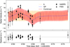 |
Fig. 7 Measured RV variation of K2-141 from HARPS (circles) and FIES (triangles). The red solid line is the best-fit model including the signal of planet b and the GP model of the correlated stellar noise. The yellow dashed line shows the signal ofplanet b. The blue dotted line shows the GP. |
7 Discussion
The three techniques used to determine the mass of K2-141 b give results that are consistent to within ~ 0.5σ. While we have no reason to prefer one method over the other, we adopted the results of M1 (FCO method), which gives a planetary mass of Mp = 5.31 ± 0.46M⊕ (~11σ significance). Figure 8 displays the K2 and RV measurements along with the inferred transit and Keplerian models from the FCO method folded to the orbital period of the planet. The parameter estimates are given in Table 3.
The upper panel of Fig. 9 shows the mass-period diagram for all the USP planets with directly measured masses. We included 55 Cnc e, CoRoT-7 b, HD 3167 b, K2-106 b, Kepler-10 b, Kepler-78 b and EPIC 228732031 b using the planetary masses and radii reported in the TEPCat database6. With a period of 0.28 d (6.7 h), K2-141 b is the shortest-period planet with a measured mass among all planets known to date. As of October 2017, there are only three transiting exoplanets known to have orbital periods shorter than K2-141 b, namely, Kepler 70 b, KOI-1843 b, and EPIC 228813918 b. However, their masses have not yet been measured. The mass of Kepler 70 b (P = 0.24 d; Charpinet et al. 2011)was estimated based on the radius and an assumed mean density. For KOI-1843 b (P = 0.18 d), the mass was constrained based on the lower limit of the planet’s mean density calculated from the requirement that the planet must orbit outside the star’s Roche limit (Rappaport et al. 2013). For EPIC 228813918 b (P = 0.18 d) Smith et al. (2018) reported a lower limit for the planetary mass based on Rappaport et al. (2013), as well as a 3σ upper limit based on RV measurements.
The mass of Mp = 5.31 ± 0.46M⊕ and radius of Rp = 1.54+0.10 −0.09 R⊕ yield a mean density of ρp = 8.00+1.83 −1.45 g cm−3. The lower panel of Fig. 9 shows the mass-radius diagram for USP small transiting planets (Porb < 1 day, Rp < 2 R⊕), along with Zeng et al. (2016)’s theoretical models for different compositions. (Dressing et al. 2015) suggested that planets with masses between 1 and 6 M⊕ are consistent with a composition of 17% Fe and 83% MgSiO3 (rock). Their sample included three USP planets (Kepler-78 b, Kepler-10 b and CoRoT-7 b), two planets with periods 4.3 and 13.8 days, and the solar system planets Earth and Venus. Figure 9 shows a 20% Fe and 80% MgSiO3 composition line, similar to the values found by Dressing et al. (2015). Given its mass and radius, K2-141 b lies close to the 40%Fe–60% MgSiO3 compositional model. Within the 1σ uncertainties, K2-141 b lies between the 20%Fe–80% MgSiO3 and 60%Fe–40% MgSiO3 models. If we consider only the five USP planets with Mp < 6 M⊕, we found that no single theoretical curve is consistent with them all. At face value this shows that there is some dispersion in the composition of USP planets.
We further inferred the composition of K2-141 b using a ternary plot (Fig. 10) for planetary compositions comprising different abundances of H2O, MgSiO3 and Fe (Zeng & Sasselov 2013; Zeng et al. 2016). The dashed lines mark the allowed region for K2-141 b, given the 1σ uncertainty on the planetary mass and radius. We first analyzed a water-free model (right-hand side of the triangle). If the planet does not contain H2 O, K2-141 b has a composition comprising ~5–70% iron and ~30–95% rocks. If the planet does contain H2O, then the maximum water abundance (1σ upper limit) cannot exceed ~30% of the total mass.
Using precise radii for 2024 Kepler planets with Porb < 100 d, Fulton et al. (2017) found a deficit of objects with 1.5 ≲Rp ≲ 2 R⊕. This gap divides close-in small planets into two distinct classes: one population comprises planets with Rp ≲ 1.5 R⊕, the other sub-Neptunes with 2 ≲Rp ≲ 3.0 R⊕. Theoretical models suggest that the observed gap might be due to photo-evaporation (e.g., Lopez & Fortney 2014; Owen & Wu 2013). According to these models, close-in (a ≲ 0.1 AU) planets in the sub-Neptunes regime would lose their atmosphere within a few hundred Myr due to the intense level of photo-ionizing radiation from their host stars, forming bare rocky cores. K2-141 b receives a stellar radiation of about 2900 F⊕ (where F⊕ refers to insolation received on Earth), which is more than four times the threshold of 650 F⊕ needed for planets to undergo photo-evaporation of H/He envelopes (Lundkvist et al. 2016). This implies that if K2-141 b had an atmosphere, it was lost due to the vicinity to its host star.
Rappaport et al. (2013) pointed out that for planets with orbital periods ≲ 6 h, the mere requirement that the planet is outside the Roche limit leads to an astrophysically relevant lower limit on the planet’s mean density. Assuming a constant density, a planet with a period of 6.7 h would need a minimum density of ~ 3.5 g cm−3 to avoid tidal destruction by the star. This value is smaller than K2-141 b’s density lower limit of 5.2 g cm−3. In this case the RV data are more powerful than the Roche-limit consideration, for determining the planet’s composition.
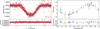 |
Fig. 8 Left panel: transit light curve folded to the orbital period of K2-141 b and residuals. The red points mark the K2 data, whereas the thick black line the re-binned best-fitting transit model. Right panel: phase-folded RV curve of K2-141 folded to the orbital period of the planet, as obtained using the FCO method. The best fitting circular solution is marked with a solid black line. HARPS and FIES data are shown with filled circles and squares, respectively. Different colors refer to different nights. Lower panels: the residuals to the best fitting model. |
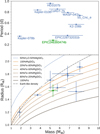 |
Fig. 9 Mass-period (upper panel) and mass-radius (lower panel) diagram for USP planets (Porb < 1 day, Rp < 2 R⊕) with measured masses. The solid green circle marks the position of K2-141 b. USP planets in the literature are marked with blue squares. The composition models from Zeng et al. (2016) are displayed with different lines and colors. The Earth-like density curve is also shown with a dot-dashed black line. |
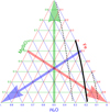 |
Fig. 10 Ternary plot for different planetary compositions. We show different combinations of water, rock and iron for possible solid planet compositions. The solid and dashed black lines mark the possible position of K2-141 b and the 68% credible intervals. This plot was created using the applet available at https://www.cfa.harvard.edu/~lzeng/manipulateplanet.html. |
8 Conclusions
We present the discovery and characterization of K2-141 b, an USP planet transiting an active K7 V star in K2 campaign 12. The relatively low stellar mass (M⋆ = 0.662 ± 0.022M⊙) and the ultra short orbital period (Porb = 6.7 h), along with our multi-visit observing strategy, allowed us to detect the Doppler reflex motion of the star with a significance of about 11σ. With a mass of Mp = 5.31 ± 0.46M⊕, K2-141 b is the planet with the shortest orbital period and a measured mass known to date.
The planetary density is consistent with a composition made of a mixture of iron and rocks. We estimated that the iron content of K2-141 b cannot exceed ~70% of the total planetary mass.
Acknowledgements
We are very grateful to the NOT and ESO staff members for their unique and superb support during the observations. Data presented herein were obtained at the WIYN Observatory from telescope time allocated to NN-EXPLORE through the scientific partnership of the National Aeronautics and Space Administration, the National Science Foundation, and the National Optical Astronomy Observatory, obtained as part of an approved NOAO observing program (P. I. Livingston, proposal ID 2017B-0334). NESSI was built at the Ames Research Center by Steve B. Howell, Nic Scott, Elliott P. Horch, and Emmett Quigley. D. G. gratefully acknowledges the financial support of the Programma Giovani Ricercatori – Rita Levi Montalcini – Rientro dei Cervelli (2012) awarded by the Italian Ministry of Education, Universities and Research (MIUR). This work is partly financed by the Spanish Ministry of Economics and Competitiveness through projects ESP2014-57495-C2-1-R and ESP2016-80435-C2-2-R. M. F. and C. M. P. acknowledge generous support from the Swedish National Space Board. Sz. Cs. thanks the Hungarian OTKA Grant K113117. This paper includes data collected by the Kepler mission. Funding for the Kepler mission is provided by the NASA Science Mission directorate. This work has made use of data from the European Space Agency (ESA) mission Gaia (https://www.cosmos.esa.int/gaia), processed by the Gaia Data Processing and Analysis Consortium (DPAC; https://www.cosmos.esa.int/web/gaia/dpac/consortium). Funding for the DPAC has been provided by national institutions, in particular the institutions participating in the Gaia Multilateral Agreement. This publication makes use of VOSA, developed under the Spanish Virtual Observatory project supported from the Spanish MICINN through grant AyA2011-24052.
Note added in proof. K2-141b has also been independently discovered, confirmed, and characterized by Malavolta et al. (2018). Their results are in very good agreement with those presented here.
References
- Angus, R., Aigrain, S., Foreman-Mackey, D., & McQuillan, A. 2015, MNRAS, 450, 1787 [NASA ADS] [CrossRef] [Google Scholar]
- Baraffe, I., Homeier, D., Allard, F., & Chabrier, G. 2015, A&A, 577, A42 [NASA ADS] [CrossRef] [EDP Sciences] [Google Scholar]
- Barragán, O., Grziwa, S., Gandolfi, D., et al. 2016, AJ, 152, 193 [NASA ADS] [CrossRef] [Google Scholar]
- Barragán, O., Gandolfi, D., & Antoniciello, G. 2017, Astrophysics Source Code Library [record ascl:1707.003] [Google Scholar]
- Barragán, O., Gandolfi, D., Smith, A. M. S., et al. 2018, MNRAS, 475, 1765 [Google Scholar]
- Bayo, A., Rodrigo, C., Barrado y Navascués, D., et al. 2008, A&A, 492, 277 [NASA ADS] [CrossRef] [EDP Sciences] [Google Scholar]
- Buchhave, L. A., & Latham, D. W. 2015, ApJ, 808, 187 [NASA ADS] [CrossRef] [Google Scholar]
- Buchhave, L. A., Latham, D. W., Johansen, A., et al. 2012, Nature, 486, 375 [NASA ADS] [Google Scholar]
- Cardelli, J. A., Clayton, G. C., & Mathis, J. S. 1989, ApJ, 345, 245 [NASA ADS] [CrossRef] [Google Scholar]
- Charpinet, S., Fontaine, G., Brassard, P., et al. 2011, Nature, 480, 496 [NASA ADS] [CrossRef] [PubMed] [Google Scholar]
- Cutri, R. M., Skrutskie, M. F., van Dyk, S., et al. 2003, 2MASS All Sky Catalog of Point Sources [Google Scholar]
- Cutri, R. M., Wright, E. L., Conrow, T. et al. 2013, VizieR Online Data Catalog: II/328 [Google Scholar]
- Dai, F., Winn,J. N., Gandolfi, D., et al. 2017, AJ, 154, 226 [NASA ADS] [CrossRef] [Google Scholar]
- DENIS Consortium. 2005, VizieR Online Data Catalog; II/263 [Google Scholar]
- Dressing, C. D., Charbonneau, D., Dumusque, X., et al. 2015, ApJ, 800, 135 [NASA ADS] [CrossRef] [Google Scholar]
- Dumusque, X., Boisse, I., & Santos, N. C. 2014a, ApJ, 796, 132 [NASA ADS] [CrossRef] [Google Scholar]
- Dumusque, X., Bonomo, A. S., Haywood, R. D., et al. 2014b, ApJ, 789, 154 [NASA ADS] [CrossRef] [Google Scholar]
- Fabricius, C., Bastian, U., Portell, J., et al. 2016, A&A, 595, A3 [NASA ADS] [CrossRef] [EDP Sciences] [Google Scholar]
- Fisher, R. 1925, Statistical Methods for Research Workers (Edinburgh Oliver & Boyd) [Google Scholar]
- Foreman-Mackey, D., Hogg, D. W., Lang, D., & Goodman, J. 2013, PASP, 125, 306 [CrossRef] [Google Scholar]
- Frandsen, S., & Lindberg, B. 1999, in Astrophysics with the NOT, ed. H. Karttunen, & V. Piirola (Piikkio: Univ. Turku), 71 [Google Scholar]
- Fridlund, M., Gaidos, E., Barragán, O., et al. 2017, A&A, 604, A16 [NASA ADS] [CrossRef] [EDP Sciences] [Google Scholar]
- Fulton, B. J., Petigura, E. A., Howard, A. W., et al. 2017, AJ, 154, 109 [NASA ADS] [CrossRef] [Google Scholar]
- Gaia Collaboration (Brown, A. G. A., et al.) 2016, A&A, 595, A2 [NASA ADS] [CrossRef] [EDP Sciences] [Google Scholar]
- Gandolfi, D., Alcalá, J. M., Leccia, S., et al. 2008, ApJ, 687, 1303 [NASA ADS] [CrossRef] [Google Scholar]
- Gandolfi, D., Parviainen, H., Deeg, H. J., et al. 2015, A&A, 576, A11 [NASA ADS] [CrossRef] [EDP Sciences] [Google Scholar]
- Gandolfi, D., Barragán, O., Hatzes, A. P., et al. 2017, AJ, 154, 123 [NASA ADS] [CrossRef] [Google Scholar]
- Gray, D. F. 2008, The Observation and Analysis of Stellar Photospheres (Cambridge, UK: Cambridge University Press) [Google Scholar]
- Grunblatt, S. K., Howard, A. W., & Haywood, R. D. 2015, ApJ, 808, 127 [NASA ADS] [CrossRef] [Google Scholar]
- Guenther, E. W., Barragan, O., Dai, F., et al. 2017, A&A, 608, A93 [NASA ADS] [CrossRef] [EDP Sciences] [Google Scholar]
- Hatzes, A. P., Fridlund, M., Nachmani, G., et al. 2011, ApJ, 743, 75 [NASA ADS] [CrossRef] [Google Scholar]
- Haywood, R. D., Collier Cameron, A., Queloz, D., et al. 2014, MNRAS, 443, 2517 [NASA ADS] [CrossRef] [Google Scholar]
- Høg, E., Fabricius, C., Makarov, V. V., et al. 2000, A&A, 355, L27 [NASA ADS] [Google Scholar]
- Howell, S. B., Everett, M. E., Sherry, W., Horch, E., & Ciardi, D. R. 2011, AJ, 142, 19 [NASA ADS] [CrossRef] [EDP Sciences] [Google Scholar]
- Johnson, M. C., Gandolfi, D., Fridlund, M., et al. 2016, AJ, 151, 171 [NASA ADS] [CrossRef] [Google Scholar]
- Kipping, D. M. 2010, MNRAS, 408, 1758 [NASA ADS] [CrossRef] [Google Scholar]
- Kipping, D. M. 2013, MNRAS, 435, 2152 [Google Scholar]
- Kovács, G., Zucker, S., & Mazeh, T. 2002, A&A, 391, 369 [NASA ADS] [CrossRef] [EDP Sciences] [Google Scholar]
- Kurucz, R. L. 2013, Astrophysics Source Code Library [record ascl:1303.024] [Google Scholar]
- Lenz, P., & Breger, M. 2004, in The A-Star Puzzle, eds. J. Zverko, J. Ziznovsky, S. J. Adelman, & W. W. Weiss, IAU Symposium, 224, 786 [Google Scholar]
- Lopez, E. D., & Fortney, J. J. 2014, ApJ, 792, 1 [NASA ADS] [CrossRef] [Google Scholar]
- López-Morales, M., Haywood, R. D., Coughlin, J. L., et al. 2016, AJ, 152, 204 [NASA ADS] [CrossRef] [Google Scholar]
- Lundkvist, M. S., Kjeldsen, H., Albrecht, S., et al. 2016, Nat. Commun., 7, 11201 [Google Scholar]
- Malavolta, L., Mayo, A. W., Louden, T., et al. 2018, AJ, 155, 107 [NASA ADS] [CrossRef] [Google Scholar]
- Mandel, K., & Agol, E. 2002, ApJ, 580, L171 [NASA ADS] [CrossRef] [Google Scholar]
- Mayor, M., Pepe, F., Queloz, D., et al. 2003, The Messenger, 114, 20 [NASA ADS] [Google Scholar]
- McQuillan, A., Mazeh, T., & Aigrain, S. 2014, ApJS, 211, 24 [NASA ADS] [CrossRef] [MathSciNet] [Google Scholar]
- Narita, N., Fukui, A., Kusakabe, N., et al. 2015, J. Astron. Telesc. Instrum. Syst., 1, 045001 [NASA ADS] [CrossRef] [Google Scholar]
- Narita, N., Hirano, T., Fukui, A., et al. 2017, PASJ, 69, 29 [NASA ADS] [CrossRef] [Google Scholar]
- Nespral, D., Gandolfi, D., Deeg, H. J., et al. 2017, A&A, 601, A128 [NASA ADS] [CrossRef] [EDP Sciences] [Google Scholar]
- Ofir, A. 2014, A&A, 561, A138 [NASA ADS] [CrossRef] [EDP Sciences] [Google Scholar]
- Owen, J. E., & Wu, Y. 2013, ApJ, 775, 105 [Google Scholar]
- Pecaut, M. J.,& Mamajek, E. E. 2013, ApJS, 208, 9 [NASA ADS] [CrossRef] [Google Scholar]
- Pepe, F., Cameron, A. C., Latham, D. W., et al. 2013, Nature, 503, 377 [NASA ADS] [CrossRef] [PubMed] [Google Scholar]
- Piskunov, N., & Valenti, J. A. 2017, A&A, 597, A16 [NASA ADS] [CrossRef] [EDP Sciences] [Google Scholar]
- Rappaport, S., Sanchis-Ojeda, R., Rogers, L. A., Levine, A., & Winn, J. N. 2013, ApJ, 773, L15 [NASA ADS] [CrossRef] [Google Scholar]
- Sanchis-Ojeda, R., Rappaport, S., Winn, J. N., et al. 2014, ApJ, 787, 47 [NASA ADS] [CrossRef] [Google Scholar]
- Sanchis-Ojeda, R., Rappaport, S., Pallè, E., et al. 2015, ApJ, 812, 112 [NASA ADS] [CrossRef] [Google Scholar]
- Smith, A. M. S., Gandolfi, D., Barragán, O., et al. 2017, MNRAS, 464, 2708 [NASA ADS] [CrossRef] [Google Scholar]
- Smith, A. M. S., Cabrera, J., Csizmadia, S., et al. 2018, MNRAS, 474, 5523 [NASA ADS] [CrossRef] [Google Scholar]
- Telting, J. H., Avila, G., Buchhave, L., et al. 2014, Astron. Nachr., 335, 41 [NASA ADS] [CrossRef] [Google Scholar]
- Torres, G. 2010, AJ, 140, 1158 [NASA ADS] [CrossRef] [Google Scholar]
- Torres, G., Andersen, J., & Giménez, A. 2010, A&ARv, 18, 67 [Google Scholar]
- Valenti, J. A.,& Fischer, D. A. 2005, ApJS, 159, 141 [NASA ADS] [CrossRef] [MathSciNet] [Google Scholar]
- Valenti, J. A.,& Piskunov, N. 1996, A&AS, 118, 595 [NASA ADS] [CrossRef] [EDP Sciences] [Google Scholar]
- Van Eylen, V., Agentoft, C., Lundkvist, M. S., et al. 2017, MNRAS, submitted, [arXiv:1710.05398] [Google Scholar]
- Vanderburg, A., & Johnson, J. A. 2014, PASP, 126, 948 [NASA ADS] [CrossRef] [Google Scholar]
- Winn, J. N., Sanchis-Ojeda, R., Rogers, L., et al. 2017, AJ, 154, 60 [NASA ADS] [CrossRef] [Google Scholar]
- Yee, S. W., Petigura, E. A., & von Braun, K. 2017, ApJ, 836, 77 [NASA ADS] [CrossRef] [Google Scholar]
- Zeng, L., & Sasselov, D. 2013, PASP, 125, 227 [NASA ADS] [CrossRef] [Google Scholar]
- Zeng, L., Sasselov, D. D., & Jacobsen, S. B. 2016, ApJ, 819, 127 [NASA ADS] [CrossRef] [Google Scholar]
Following Fisher (1925), we adopted a significance level of p = 0.05.
All Tables
Main identifiers, coordinates, optical and infrared magnitudes, and proper motion of K2-141.
All Figures
|
Fig. 1 K2 light curve of K2-141. Stellar activity is seen as the quasi-periodic, long period modulation. Transits are visible as shallow dips. The 5.3-day-long data gap, during which the telescope entered safe mode, is clearly visible at approximately two-thirds of the way through the time series. |
| In the text | |
|
Fig. 2 “Blue” and “red” contrast curves and reconstructed images of K2-141 (insets). The two images are both centered around K2-141 and have a size of 4.6″× 4.6″. |
| In the text | |
|
Fig. 3 Spectral energy distribution of K2-141. The BT-Settl-CIFIST model spectrum with the same parameters as the star is plotted with a light blue line. The V J, IC, J, H, Ks, W1, W2, W3, and W4 fluxes are derived from the magnitudes reported in Table 1. |
| In the text | |
|
Fig. 4 Cores of the Ca II H & K lines of K2-141 as observed with HARPS. |
| In the text | |
|
Fig. 5 Discrete Fourier transform of the HARPS RV measurements. The dashed red line marks the frequency at the orbital period of K2-141 b. |
| In the text | |
|
Fig. 6 Upper panel: HARPS RV residuals following the subtraction of the transiting planet signal vs. time. Lower panels: Ca II H&K S activity index (top), cross-correlation FWHM (middle), and cross-correlation bisector span (bottom) vs. RV residuals. The dashed red lines mark the best fitting linear fit. |
| In the text | |
|
Fig. 7 Measured RV variation of K2-141 from HARPS (circles) and FIES (triangles). The red solid line is the best-fit model including the signal of planet b and the GP model of the correlated stellar noise. The yellow dashed line shows the signal ofplanet b. The blue dotted line shows the GP. |
| In the text | |
|
Fig. 8 Left panel: transit light curve folded to the orbital period of K2-141 b and residuals. The red points mark the K2 data, whereas the thick black line the re-binned best-fitting transit model. Right panel: phase-folded RV curve of K2-141 folded to the orbital period of the planet, as obtained using the FCO method. The best fitting circular solution is marked with a solid black line. HARPS and FIES data are shown with filled circles and squares, respectively. Different colors refer to different nights. Lower panels: the residuals to the best fitting model. |
| In the text | |
|
Fig. 9 Mass-period (upper panel) and mass-radius (lower panel) diagram for USP planets (Porb < 1 day, Rp < 2 R⊕) with measured masses. The solid green circle marks the position of K2-141 b. USP planets in the literature are marked with blue squares. The composition models from Zeng et al. (2016) are displayed with different lines and colors. The Earth-like density curve is also shown with a dot-dashed black line. |
| In the text | |
|
Fig. 10 Ternary plot for different planetary compositions. We show different combinations of water, rock and iron for possible solid planet compositions. The solid and dashed black lines mark the possible position of K2-141 b and the 68% credible intervals. This plot was created using the applet available at https://www.cfa.harvard.edu/~lzeng/manipulateplanet.html. |
| In the text | |
Current usage metrics show cumulative count of Article Views (full-text article views including HTML views, PDF and ePub downloads, according to the available data) and Abstracts Views on Vision4Press platform.
Data correspond to usage on the plateform after 2015. The current usage metrics is available 48-96 hours after online publication and is updated daily on week days.
Initial download of the metrics may take a while.