| Issue |
A&A
Volume 612, April 2018
|
|
|---|---|---|
| Article Number | A84 | |
| Number of page(s) | 12 | |
| Section | The Sun | |
| DOI | https://doi.org/10.1051/0004-6361/201732118 | |
| Published online | 01 May 2018 | |
Mapping the solar wind HI outflow velocity in the inner heliosphere by coronagraphic ultraviolet and visible-light observations★
1
INAF–Catania Astrophysical Observatory,
Via Santa Sofia 78,
95123
Catania, Italy
e-mail: This email address is being protected from spambots. You need JavaScript enabled to view it.
2
INAF–Turin Astrophysical Observatory,
Via Osservatorio 20,
10025
Pino Torinese (TO), Italy
3
INAF–Capodimonte Astronomical Observatory,
Salita Moiariello 16,
80131
Napoli, Italy
4
CNR–Institute of Photonics and Nanotechnologies,
Via Trasea 7,
35131
Padova, Italy
5
INAF–Arcetri Astrophysical Observatory,
Largo Enrico Fermi 5,
50125
Firenze, Italy
6
University of Padova–Dept. of Physics and Astronomy,
Via Marzolo 8,
35131
Padova, Italy
7
University of Padova–Dept. of Information Engineering,
Via Gradenigo 6/B,
35131
Padova, Italy
8
University of Firenze–Dept. of Physics and Astronomy,
Largo Enrico Fermi 2,
50125
Firenze, Italy
Received:
17
October
2017
Accepted:
27
December
2017
Abstract
We investigated the capability of mapping the solar wind outflow velocity of neutral hydrogen atoms by using synergistic visible-light and ultraviolet observations. We used polarised brightness images acquired by the LASCO/SOHO and Mk3/MLSO coronagraphs, and synoptic Lyα line observations of the UVCS/SOHO spectrometer to obtain daily maps of solar wind H I outflow velocity between 1.5 and 4.0 R⊙ on the SOHO plane of the sky during a complete solar rotation (from 1997 June 1 to 1997 June 28). The 28-days data sequence allows us to construct coronal off-limb Carrington maps of the resulting velocities at different heliocentric distances to investigate the space and time evolution of the outflowing solar plasma. In addition, we performed a parameter space exploration in order to study the dependence of the derived outflow velocities on the physical quantities characterising the Lyα emitting process in the corona. Our results are important in anticipation of the future science with the Metis instrument, selected to be part of the Solar Orbiter scientific payload. It was conceived to carry out near-sun coronagraphy, performing for the first time simultaneous imaging in polarised visible-light and ultraviolet H I Lyα line, so providing an unprecedented view of the solar wind acceleration region in the inner corona.
Key words: Sun: corona / solar wind / Sun: UV radiation
The movie (see Sect. 4.2) is available at https://www.aanda.org
© ESO 2018
1 Introduction
The solar wind is a flow of a tenuous solar plasma escaping from the sun and pervading the interplanetary space. The origin of this flow is primarily due to the huge difference in gas pressure between the very hot solar corona and the interplanetary space. The importance of studying the solar wind stands in two major points: the role it plays on the influence of the terrestrial environment and the basic physical processes concerning its formation and expansion. New technologies of the forthcoming missions to the sun will contribute to enhance the current knowledge of the solar wind. Solar Orbiter (Müller et al. 2013), in particular, is a medium-class mission scheduled for launch in February 2019 by the European Space Agency (ESA), whose aim is to study the sun and the inner heliosphere thanks to an innovative scientific payload and a new orbital approach. The Metis coronagraph (Antonucci et al. 2012) will be one of the instruments aboard the Solar Orbiter spacecraft and it is designed to exploit the characteristic of the mission profile. It will give a unique contribution to answer the scientific questions of the mission, such as acceleration of the solar energetic particles, onset and early propagation of coronal mass ejections (CMEs), and origin and acceleration of the solar wind. Metis will acquire for the first time simultaneous coronagraphic images of the inner heliosphere in broad-band (580–640 nm) polarised visible-light (VL) and narrow-band (121.6 ± 10 nm) ultraviolet (UV) H I Lyα line, providing an unprecedented view of the solar wind acceleration region with a high temporal coverage and a spatial resolution down to about 4000 km for the spacecraft at the perihelion. The field of view (FOV) will span over a wide range owing to the Solar Orbiter orbit, so observing from 1.6 to 7.5 R⊙.
In this perspective, we investigated the capability of mapping the solar wind outflow velocity of neutral hydrogen atoms in the inner heliosphere by using synergistic coronagraphic UV and VL observations. We used observations acquired by space- and ground-based instruments, such as the UltraViolet Coronagraph Spectrometer (UVCS; Kohl et al. 1995) and the Large Angle and Spectrometric COronagraph (LASCO; Brueckner et al. 1995) aboard the SOlar and Heliospheric Observatory (SOHO; Domingo et al. 1995), and the Mark-III K-Coronameter (Mk3; Fisher et al. 1981) installed at the Mauna Loa Solar Observatory (MLSO). We selected data over a time interval of 28 days in June 1997, covering a complete solar rotation, and reconstructed UV and VL full-corona images in the range of heliocentric distances between 1.5 and 6.0 R⊙. We then synthesised the coronal H I Lyα line intensity by deriving electron densities from the VL images and using physical quantities reported in the literature, and finally compared the result with the observed UV Lyα intensity. Since the coronal UV intensity of the Lyα line is depending not only on the electron density but also on the plasma outflow speed, we applied the Doppler dimming technique (see e.g. Withbroe et al. 1982) and derived daily H I outflow velocity maps in the altitude range 1.5–4.0 R⊙ on the SOHO plane of the sky (hereafter POS). The 28-days data sequence allows us to construct coronal off-limb Carrington maps of the outflow velocity of the solar wind at different heliocentric distances to analyse the evolution of the outflowing plasma propagation in the inner heliosphere during a solar rotation and, in particular, to investigate possible north-south pole asymmetries in the speed values. In the end, we presented a critical discussion on the quantities adopted in the synthesis of Lyα line intensity and studied the dependence of the resulting solar wind H I outflow velocity on the physical parameters characterising the Lyα emitting process in the corona through a parameter space exploration.
To derive the H I ouflow speed, by matching the observed UV Lyα line intensity and that modelled on the basis of the coronal electron density, we performed the synthesis of the Lyα line along the line of sight (LOS). Our technique is potentially suitable to take into account also effects such as H I temperature anisotropies and inhomogeneities in the distribution of the exciting chromospheric radiation. The inclusion of such effects will be important for a careful analysis of the Metis UV data. Furthermore we discussed the impact of parametrization of different quantities that will be assumed in the analysis of the future coronagraphic observations. In this work we focused only on the characteristics of the H I speeds derived above 1.5 R⊙, lower limit of the FOV of Metis as well as of the FOV covered by UVCS during the daily synoptic observations. The same dataset has been analysed by Bemporad (2017), but with a different method and different purposes. Bemporad derived the H I outflow speeds with a simplified technique that neglects LOS integration effects (see Sect. 4.2) and focuses mostly on the radial evolution of the outflow velocity in the inner part of the corona, extrapolating the UVCS data below 1.5 R⊙, also discussing possible physical explanations for a deceleration and subsequent acceleration of the solar wind resulting from his analysis.
2 H I Lyα line radiation in the solar corona
The emission of the H I Lyα line in a static solar corona is due to two mechanisms: 1) collisional excitation by free electrons impact and 2) resonant scattering of chromospheric radiation by neutral hydrogen atoms, with the first one accounting only for a small fraction to the total emission of the radiative process (Gabriel 1971; Raymond et al. 1997). Intensity of the resonantly scattered Lyα line coming from a coronal point P and measured by an observer in the direction n depends on geometrical and physical parameters according to the following functional form (see e.g. Dolei et al. 2015; Noci et al. 1987; Noci & Maccari 1999):
 (1)
(1)
where λ0 = 121.6 nm is the central wavelength of the Lyα line profile,  is the specific intensity of chromospheric radiation at wavelength λ′ propagating in the direction n′ and incidenton P, Ω is the solid angle under which the point P subtends the solar disk, ne is the coronal electron density, Te is the coronal electron temperature, and THI is the temperature of the coronal neutral hydrogen atoms giving rise to the coronal absorption profile centred at λ0. It is worth noting that THI contains both the thermal component and that due to plasma flows and waves, and is generally assumed isotropic, although it can be anisotropic in coronal structures, such as coronal holes (see e.g. Dolei et al. 2016; Telloni et al. 2007). The last parameter vw is the outflow velocity of the scattering H I atom in P due to the solar wind.
Outward expansion of coronal plasma causes a reduction in intensity of the scattered Lyα line. In fact, when the corona is in a static condition, the profile of the chromospheric Lyα radiation incident on the corona and the absorption profile of the scattering H I atoms are centred at the same wavelength λ0. This produces the maximum intensity of the resonantly scattered Lyα line. Conversely, when the corona expands with a certain outflow velocity, the incident radiation profile appears to be Doppler-shifted in the rest frame of the scattering atoms. The rate of resonant scattering process decreases until approaching to zero when the outflow velocity increases to a high values such that the chromospheric and coronal absorption profiles do not overlap anymore. The progressive reduction (or dimming) in intensity of the resonantly scattered Lyα line with the increasing solar wind H I outflow velocity is called the Doppler dimming effect (Hyder & Lytes 1970; Noci et al. 1987; Withbroe et al. 1982). The Doppler dimming technique exploits this effect to derive the H I outflow velocity of the expanding coronal plasma through the comparison between the intensity, as a function of vw, that can be synthesised according to Eq. (1) and the intensity measured by means of UV Lyα line observations. The synthetic intensity can be obtained by tuning the value of the H I outflow speed in order to reproduce the observations. In so doing, the match between synthetic and observed Lyα line intensity provides an estimate of the solar wind H I outflow velocity.
We defined as the effective Doppler dimming coefficient the synthetic intensity ratio
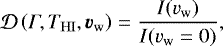 (2)
where vw is the modulus of the vw vector. Such a coefficient is only sensitive to the geometrical properties of the Lyα resonant scattering process (Γ), and to the values of temperature and velocity of the scattering H I atoms along the LOS. Figure 1 shows the effective Doppler dimming coefficient calculated at the heliocentric distance r = 2.5 R⊙, on the plane of the sky of the observer, fora polar coronal hole with THI = 2.2 MK averaged along the LOS, and r = 4.0 R⊙ for an equatorial streamer with THI = 1.6 MK averaged along the LOS. We considered these two curves as representative of the
(2)
where vw is the modulus of the vw vector. Such a coefficient is only sensitive to the geometrical properties of the Lyα resonant scattering process (Γ), and to the values of temperature and velocity of the scattering H I atoms along the LOS. Figure 1 shows the effective Doppler dimming coefficient calculated at the heliocentric distance r = 2.5 R⊙, on the plane of the sky of the observer, fora polar coronal hole with THI = 2.2 MK averaged along the LOS, and r = 4.0 R⊙ for an equatorial streamer with THI = 1.6 MK averaged along the LOS. We considered these two curves as representative of the  values in the polar and equatorial regions, respectively. The plot points out that the Lyα line is significantly reduced in intensity with respect to the static condition for outflow velocities higher than 100 km s−1 and appears to be almost completely dimmed for vw > 450 km s−1. In particular, a reduction in intensity by a factor of 3% occurs for vw = 50–60 km s−1.
We also calculated the absolute value of the derivative of the effective Doppler dimming coefficient with respect to vw ( , see Fig. 1), which expresses the variation rate of
  . The results indicate that, for instance, around the maximum value of the red dashed curve, corresponding to an outflow velocity of about 200 km s−1, a speed variation of 10 km s−1 is sufficient to cause a variation of
  by a factor of 3%. Conversely, for derivative values corresponding to outflow velocities lower than 50 km s−1 or higher than 450 km s−1 (below the horizontal black dotted line), a speed variation of at least 30 km s−1 is necessary to cause the same 3%
  variation. Hence, analysis of the effective Doppler dimming coefficient as a function of heliocentric distance and H I temperature allows us to infer the range of uncertainty affecting the measurements of solar wind H I outflow velocity that can be obtained through the Doppler dimming technique.
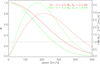 |
Fig. 1 Effective Doppler dimming coefficient of the resonantly scattered H I Lyα line (solid lines) and absolute value of its derivative with respect to the outflow speed (dashed lines), calculated at the heliocentric distance r = 2.5 R⊙, on the plane of the sky of the observer, for a polar coronal hole (CH) with THI = 2.2 MK averaged along the LOS (red lines), and r = 4.0 R⊙ for an equatorial streamer (STR) with THI = 1.6 MK averaged along the LOS (green lines). |
3 Observations
We selected data acquired at the same time, or approximately, by three instruments in order to reconstruct simultaneous images of the same coronal region in both UV and VL spectral bands and simulate the future observations with the Metis coronagraph. We investigated the UVCS/SOHO, LASCO/SOHO, and Mk3/MLSO catalogues to select a time interval of 28 days at least with a continuous coverage of UVCS daily synoptic observations, and LASCO and Mk3 polarised brightness images. The UVCS synoptic observations were acquired each day over a time interval of about 10–12 h, though unevenly spaced in time, and can be considered as representative of the average Lyα line emission of the scanned solar corona over the whole day. The VL polarised brightness images acquired by LASCO and Mk3 were selected, accordingly, to minimise the time gap with the UV observations. Our aim was to use the UV and VL data to derive solar wind HI outflow velocities on the POS during a complete solar rotation. Despite the large amount of archived data, our research was confined to the time interval from the 1st to the 28th June 1997, because of the discontinuous coverage of the UVCS observations. The solar magnetic activity in June 1997 was almost at the minimum phase between the cycles 22 and 23, and the coronal structures (such as streamers, coronal holes, plumes) appear to be well outlined. Hence, the selected data turn out to be suitable for studying the solar wind dynamics and discriminate sources of fast and slow outflows.
3.1 UV data processing
The UVCS/SOHO synoptic spectrometric observations consist of raster scans of the full corona at eight different angular positions separated by steps of 45°. The slit of the spectrometer, whose FOV is 40 arcmin long, is parallel to a tangent to the solar limb on the POS and can be radially moved, usually covering altitudes between 1.5 and 3.5 R⊙. Slit positions in the synoptic pattern are reported in the top left panel of Fig. 2.
The 28-days sequence of the selected synoptic data was analysed by the last version of the Data Analysis and processing Software (DAS 5.1; developed by C. Benna, A. Van Ballegoijen, J. Raymond, and S. Giordano). We used suitable routines for flat-field correction, wavelength and radiometric calibration, background subtraction,as well as for the estimate and removing of the contribution of stray light and interplanetary Lyα line from the coronal H I Lyα line emission. We obtained 28 daily synoptic maps of the UV Lyα intensity in the range 1.5–3.5 R⊙ of heliocentric distance. The daily maps were, then, interpolated and extrapolated at all latitudes by a double power law to reconstruct a sequence of UV H I Lyα coronagraphic images in the altitude range from 1.5 to 6.0 R⊙, in order to overlap the outer region of the investigated LASCO field of view (see below). The bottom left panel of Fig. 2 shows the Lyα intensity image that we reconstructed from the synoptic map of the 1st June. This kind of image is what is expected from the future coronagraphic observations with the UV channel of Metis. We note that the UVCS planning programme scheduled one synoptic a day on average, with 10–12 hours of acquisition time. Conversely, Metis will acquire UV full corona images with a temporal resolution of the order of minutes.
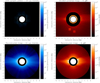 |
Fig. 2 Left panels: UV H I Lyα line intensityon the 1st June 1997, in units of photons cm−2 s−1 sr−1, as measured by the UVCS daily synoptic observation (top) and reconstructed between 1.5 and 6.0 R⊙ (bottom). Right panels: VL polarised brightness on the 1st June 1997, in units of Mean Solar Brightness (MSB), asmeasured by the LASCO C2 and Mk3 coronagraphs (top) and reconstructed between 1.5 and 6.0 R⊙ (bottom). |
3.2 VL data processing
The C2 camera of LASCO/SOHO performed VL coronagraphic observations between 2.5 and 6.5 R⊙. The LASCO archive provides up to four VL polarised brightness (pB) images a day during June 1997. We only selected the pB image temporally closer to the UVCS daily synoptic for simulating the simultaneous UV and VL imaging that will be performed by Metis. We combined the LASCO C2 pB images withthose acquired by the ground-based Mk3 of the MLSO, whose FOV goes from 1.12 to 2.44 R⊙, in order to better cover the coronal region at lower heliocentric distance. We obtained 28 daily C2+Mk3 combined images of polarised brightness, such as that shown in the top right panel of Fig. 2 that is related to the observations made on June 1. We interpolated the combined images at all latitudes by a double power law and reconstructed a sequence of pB coronagraphic images in the altitude range 1.5–6.0 R⊙. In order to minimise the errors of the image interpolation, intensities at coronal regions located at heliocentric distances lower than 1.1 R⊙ and higher than 1.5 R⊙ were excluded from the Mk3 images, as well as intensities below 2.5 R⊙ from the C2 images. The bottom right panel of Fig. 2 shows the pB image that we reconstructed from the C2+Mk3 combined image of the 1st June. Similarly to the UV images, this kind of image is what is expected from the future VL coronagraphic observations of Metis.
Since the coronal polarised brightness is only depending on the electron density through some geometrical factors (Billings 1966; Van De Hulst 1950), we used the sequence of reconstructed pB images to determine radial profiles of ne by means of the Van De Hulst inversion (Van De Hulst 1950). This technique takes into account a cylindrical symmetry with respect to sun’s rotation axis of the solar corona and assumes that the density profiles can be expressed by the polynomial form ne (r)= ∑ k(αk r−k), where r is the heliocentric distance and k is an integer varying between one and four (see e.g. Dolei et al. 2015 and Hayes et al. 2001 for a more detailed description). We used a multivariate least-squares fit to synthesise pB radial profiles and obtain the coefficients αk best reproducing the polarised brightness that we reconstructed from the VL observations. These coefficients were then substituted into the polynomial form of ne(r) to derive the electron density radial profiles, such as those shown in Fig. 3, which can be considered as representative of equatorial and polar regions between 1.5 and 6.0 R⊙. The dotted areas represent the uncertainty range of the density values (10–20%). It was determined for a ±10% variation of the polarised brightness profiles by means of the inversion technique. The pB uncertainty of 10% takes into account errors in the photometric calibration of the LASCO and MLSO instruments and in the VL image interpolation.
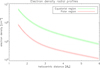 |
Fig. 3 Coronal electron density profiles in equatorial (green solid line) and polar (red solid line) regions obtained by means of the Van De Hulst inversion technique. The dotted areas represent the range of density uncertainty corresponding to a ±10% variation of the polarised brightness profiles. |
4 Synthesis of the resonantly scattered H I Lyα line intensity
The aim of this work is to test a method for mapping the solar wind H I outflow velocity in the inner heliosphere, by simulating simultaneous observations performed with UV and VL coronagraphs designed for imaging only. For our purposes, we synthesised the intensity of the resonantly scattered H I Lyα line by means of a numerical code (developed in its original form by Spadaro & Ventura 1994 and subsequently improved) that uses the functional form given by Eq. (1), assumes uniform chromospheric Lyα radiation, ionisation equilibrium in the coronal plasma, isotropic temperature of the coronal neutral hydrogen atoms, cylindrical symmetry of the solar corona, and takes into account the Doppler dimming effect on the resonantly scattered Lyα line due to the wind outflows. In the absence of specific measurements to determine all the physical parameters reported in Eq. (1), we adopted a suitable set of values as input data in the synthesis computation. In particular, we used the radial profiles of ne derived from the reconstructed pB images and data reported in the literature to establish the values of  , Te, and THI, characterising the chromospheric and coronal environments during the minimum phase of the solar magnetic activity.
4.1 Definition of the computational parameters
We adopted the chromospheric H I Lyα line profile proposed by Auchère (2005). It can be expressed as 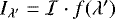 , where
  × 1015 photons cm−2 s−1 sr−1 is the chromospheric Lyα line intensity inferred from the measurements of solar disk irradiance performed in June 1997 (Lemaire et al. 2002) with the SOLar STellar Irradiance Comparison Experiment (SOLSTICE; Rottman & Woods 1994) aboard the Upper Atmosphere Research Satellite (UARS; Reber 1990), and f(λ′) represents the normalised profile shown in Fig. 4, whose analytical form is expressed by Eq. (6) in Auchère (2005).
We also selected the electron temperature radial profiles that were inferred from observations of an equatorial streamer at solar minimum by Gibson et al. (1999) and modelled for polar regions by Vasquez et al. (2003). In the hypothesis of superradial expansion of the solar wind in polar coronal holes during the minimum phase of the solar magnetic activity (Low 1990; Roberts & Goldstein 1998), we adopted the Gibson et al. (1999) profile for estimating the Te values at latitudes between − 20° and +20°, and the Vasquez et al. (2003) profile for the Te values at latitudes lower than − 40° and higher than +40° (see Fig. 5). To establish the values of Te at the mid-latitude regions, we constructed a sequence of electron temperature radial profiles by interpolating the two selected profiles at all heliocentric distances between 1.5 and 6.0 R⊙. This sequence covers the shaded area shown in Fig. 5.
Moreover, we constructed a temperature map of coronal neutral hydrogen atoms by using UVCS Lyα spectrometric observations at solar minimum that were already investigated by Dolei et al. (2016). These authors analysed a large amount of data, covering a time interval longer than a whole solar activity cycle, and constructed a reliable and statistically significant database of H I temperatures. In particular, they derived THI radial profiles for different angular positions and solar magnetic activity phases, in various altitude ranges all between 1.3 and 4.5 R⊙. In the top panel of Fig. 6 we reported the map of the THI values from 1.5 to 4.0 R⊙ obtained by Dolei et al. (2016) from observations at solar minimum. A Delaunay triangulation (Delaunay 1934) was perfomed in order to fill the voids present in the map (see Sect. 2 of Dolei et al. 2016 for a more detailed description). Then we used the functional form given by Vasquez et al. (2003) and reported in Eq. (1) of Dolei et al. (2016) to radially fit the resulting temperature profiles and, finally, we obtained the THI map shown in the bottom panel of Fig. 6. It is worth remarking that the constructed H I temperature map takes into account numerous observations covering a time interval much longer than that considered for the selection of UV and VL data used in our work.
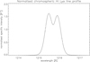 |
Fig. 4 Adopted normalised chromospheric H I Lyα line profile. |
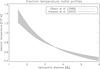 |
Fig. 5 Coronal electron temperature profiles adopted for equatorial (dotted line) and polar (dashed line) regions. The shaded area corresponds to the sequence of Te profiles usedfor the mid-latitude regions. |
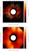 |
Fig. 6 Top panel: map of the THI values at solar minimum obtained by Dolei et al. (2016) from the analysis of the Lyα line width. Bottom panel: adopted coronal H I temperature map. |
4.2 Solarwind H I outflow velocity
Having adopted the various physical quantities reported in Eq. (1), the numerical code calculates the emissivity of the resonantly scattered H I Lyα line. In order to reproduce the observed UV Lyα line intensity, the code takes into account the Doppler dimming effect, integrates the emissivity contributions along the LOS, and provides thesynthetic intensity, tuning the outflow velocity values by means of a double numerical iteration, as described inthe following. First, zero bulk outflow velocity is assumed throughout the LOS. If the resulting synthetic H I Lyα line intensity is higher than that reconstructed from the UVCS synoptic observations, the code progressively increases the speed value to obtain a match, assuming the same increase along the LOS. The process is performed for the lines of sight intersecting a certain radial direction on the POS. At this stage, in order to obtain a more realistic outflow velocity profile along the LOS, the code uses the speed radial profile on the POS obtained in the previous step of the computation and, assuming a cylindrical symmetry of the solar corona, assigns the corresponding speed value to derive the new profile along the LOS. Then, the code re-synthesises the Lyα emissivity and integrates the emissivity contributions along the LOS to provide the synthetic intensity. The iteration process will continue tuning progressively the outflow velocity values to obtain the best match between the synthetic Lyα line intensities and the reconstructed ones.
We derived the values of the solar wind H I outflow velocity during the selected 28 days of June 1997 corresponding to a complete solar rotation. We obtained daily maps of H I outflow velocity between 1.5 and 4.0 R⊙ on the POS. This altitude range is mainly constrained by that of the adopted H I temperature map and better reflects the range of heliocentric distances directly investigated with the UVCS Lyα synoptic observations. A movie showing the evolution of the solar wind dynamics during the whole solar rotation is available online. The wide void areas in some frames of the movie are due to gaps in the UVCS synoptic data owing to telemetry problems or special spacecraft maneuvers. The time evolution shows wind streams with a quite stable latitudinal distribution in the polar regions, while rapidly changing structures are characterising the equatorial regions.
Figure 7 shows the H I outflow velocity maps of the 1997 June 1 and, half a solar rotation later, June 14 (top panels), and the speed profiles along four radial directions in the equatorial and polar regions (bottom panels). The resulting outflow velocities generally radially increase with the heliocentric distance up to about 150–200 km s−1 in the equatorial region and above 400 km s−1 in the polar regions. The steep increase of the radial profiles at lower velocities demonstrates that at such speeds a significant gradient in the coronal Lyα intensity corresponds to a large variation of the solar wind speed values (see also Fig. 1). The dotted areas in the bottom panels of Fig. 7 represent the error bars of the resulting outflow velocities that were derived as a result of an uncertainty of the reconstructed UV Lyα line intensity by a factor of 3%, according to the variation rate of the effective Doppler dimming coefficient for equatorial and polar regions (see discussion in Sect. 2). The error bars are plotted for the speed values higher than zero, but the uncertainties affect each velocity profile down to 1.5 R⊙, also where the corona turns out to be in a static condition. Our results are in agreement with the expected latitudinal distribution of slow and fast solar wind components, corresponding to equatorial regions, and mid-latitude (above 35° of latitude) and polar regions, respectively. The maps also show some tiny wind streams in the equatorial regions between 1.5 and 2.5 R⊙, with high speeds (vw > 100 km s−1) decreasing with altitude. These unexpected structures were already noticed by Bemporad (2017), who analysed the same set of data used in this work. They could be the result of averaging among several transient structures (i.e. jets) with significant flows appearing at the top, or near the boundaries, of active region closed magnetic loops (Del Zanna 2008; Harra et al. 2007) and giving some contribution to the solar wind outflows.
We also reported outflow velocity radial and latitudinal profiles over the whole investigated time interval in Fig. 8. The slow solar wind speeds (top panel) show a larger variability than the fast solar wind speeds at higher altitudes (middle panel), as confirmed by the in situ solar wind measurements (see e.g. McComas et al. 2000). In addition, the radial profiles point out no significant difference between the equatorial velocities measured above the solar east and west limbs, whereas the speeds in the northern regions result to be systematically higher than those in the southern regions. This indicates that a clear north-south pole asymmetry in the speed values occurred in June 1997, as also supported by the outflow velocity latitudinal profiles obtained at 2.5 and 3.5 R⊙, which are reported in the bottom panel of Fig. 8. Coronal plasma flows slower in the southern regions at lower altitudes and then increases its speed until almost reaching the value characterising the northern regions above 3.5 R⊙. This suggests a different magnetic field configuration between the two poles, as verified by very recent works demonstrating that globally the northern hemisphere was more active than the southern one in the middle period of 1997 (Svalgaard & Kamide 2013), and that the north coronal hole had a larger area than that of the south coronal hole (Hess Webber et al. 2014; Lowder et al. 2017). The north-south pole asymmetry appears also to extend at higher heliocentric distances, where it manifests both on large-scale solar temporal variations (McComas et al. 2000) and on short-period observations (Kojima et al. 2001). Moreover, Auchère et al. (2005), examining the behaviour of the solar flux of the heliospheric He II line emission at 30.4 nm during the activity cycle 23, noticed that the north flux was larger than the south flux, with the difference reaching about 20% in 1999 and 2000. They considered this asymmetry as a signature of the unequal distribution of active regions between the north and south hemispheres of the sun. On the other hand, we should also consider a possible dependence of the LASCO C2 pB calibration on the position angle, that could give rise to differences in the coronal polarised brightness between the north and south polar coronal holes, as pointed out by Frazin et al. (2002, 2012). This would result in different electron densities derived for the two polar coronal holes and could contribute to the appearance of a spurious north-south asymmetry in the solar wind outflow velocity. Taking into account this aspect, the observed asymmetry could decrease by a quantity that is not possible to quantify.
We used daily speed latitudinal profiles at different altitudes, such as those reported in the bottom panel of Fig. 8, to construct coronal off-limb Carrington maps of H I outflow velocity. Figure 9 shows the Carrington maps at 2.5 and 3.5 R⊙. They represent a snapshot of the time evolution of the solar wind speed on the POS at a given heliocentric distance. The 28-days sequence partially covers both the Carrington rotation numbers 1923 and 1924. The Carrington maps confirm that the asymmetry in the speed values between the north and south polar regions at lower altitudes is maintained over the 28 days. In addition, a speed increase at 2.5 R⊙ occurs fromday 19 on, while the velocity appears to keep constant at 3.5 R⊙ all over the time interval.
It is worth pointing out that the technique for the derivation of the H I outflow velocities described in this work, which is based on the self-consistent integration of the Lyα emissivity along the LOS by tuning the outflow speed in order to reach the best agreement between synthesised and observed intensity, needs the previous determination of coronal electron density profiles and various assumptions on the physical and geometrical properties characterising the chromospheric and coronal environments. An alternative technique was first suggested by G. Noci and described by Withbroe et al. (1982): since, in first approximation, the UV Lyα line and VL polarised emissions are both proportional to the integral of the coronal electron density along the LOS, the ratio between these two quantities is only sensitive to H I temperature (averaged along the LOS) and solar wind outflow velocity. Hence, once a mean value of THI is assumed, a mean outflow speed can be directly derived from the ratio between observed UV and VL intensities, avoiding the derivation of the electron density from VL data and the integration of the Lyα emissivity along the LOS, and also reducing significantly the computational time. This technique will be thus more suitable to perform quick reduction of the future Metis data and to derive quick-look H I outflow velocity maps on the plane of the sky (see more details in Bemporad 2017). Advantages and disadvantages of the two techniques will be analysed in a future work. In any case, the outflow velocity maps derived here (see Fig. 7) are in general agreement with those previously reported by Bemporad (2017) to the extent the analyses overlap, also considering the uncertainties in the speed determination that we are going to describe in detail in the next Section.
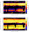 |
Fig. 9 Coronal off-limb Carrington maps of H I outflow velocity at 2.5 (top) and 3.5 R⊙ (bottom). The void areas correspond to the gaps in the UVCS synoptic data. |
5 Discussion of the results
Having verified the capability of mapping the solar wind H I outflow velocity by means of coronagraphic images, a critical discussion on the reliability of the results appears to be necessary. We investigated the dependence of the resulting outflow speeds on the physical parameters characterising the emission of the resonantly scattered Lyα line. In particular, we studied the influence of the uncertainties of the parameters ne,  , Te, and THI on the derived outflow velocities.
5.1 Physical parameter uncertainties
5.1.1 Coronal electron density
We derived the coronal electron density values by means of the Van De Hulst inversion technique (see Sect. 3.2). We also determined the range of density uncertainty for a ±10% variation of the VL polarised brightness that takes into account photometric calibration and image interpolation errors. We obtained density uncertainties ranging between 10 and 20% (see Fig. 3).
5.1.2 Exciting chromospheric Lyα line radiation
Measurements of the solar Lyα line irradiance were perfomed by the SOLSTICE instrument, with a global accuracy of 10% (Lemaire et al. 2002). To synthesise the resonantly scattered Lyα line intensity, we assumed uniform exciting chromospheric Lyα radiation on the solar disk. However, observations performed by the Solar Wind ANisotropies (SWAN; Bertaux et al. 1995) instrument aboard the SOHO spacecraft provide the evidence of anisotropy of the illumination of corona and heliosphere by the chromospheric Lyα radiation (Bertaux et al. 2000). Such anisotropy is due to the longitudinal and latitudinal distribution of bright (e.g. active regions) and dark (e.g. coronal holes) structures. Auchère (2005) evaluated the effect of anisotropy on the resonant scattering process in the corona. He found that the uniform-disk approximation leads, on average, to a systematic overestimate of the synthetic intensity of the resonantly scattered Lyα line by a factor of 15% in polar coronal holes at solar minimum. This implies an overestimate of the resulting outflow velocities in the polar regions, since a higher dimming of the synthetic intensity is necessary to match the observed coronal UV intensity. By the red curves in Fig. 1, we can note that a decrease of the effective Doppler dimming coefficient by a factor of 15% in correspondence to the maximum of its variation rate (about 200 km s−1) is obtained by a velocity increase of about 50 km s−1. This value can be considered as an average overestimate of the outflow velocity in polar regions when the radiation of the chromospheric Lyα line is assumed to be uniform on the solar disk. In addition, as discussed above, the larger area of the north coronal hole with respect to the area of the south coronal hole during 1997 (Hess Webber et al. 2014; Lowder et al. 2017) can lead to a higher overestimate of the outflow velocity in the northern coronal region, possibly contributing to the degree of north-south pole asymmetry shown in Figs. 7 and 8. In any case, the differences obtained at 2.5 R⊙ are significantly higher than 50 km s−1.
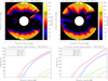 |
Fig. 7 Top panels: H I outflow velocity maps on the 1st (left) and 14th (right) June 1997. Bottom panels: H I outflow velocity radial profiles in the equatorial and polar regions on the 1st (left) and 14th (right) June 1997. The dottedareas represent the range of speed uncertainty as a result of an uncertainty of the reconstructed UV Lyα line intensity by 3%, according to the variation rate of the effective Doppler dimming coefficient. |
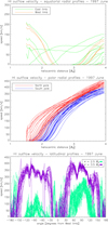 |
Fig. 8 H Ioutflow velocities over the investigated time interval: equatorial radial profiles (top); polar radial profiles (middle); latitudinal profiles (bottom) at 2.5 (cyan lines) and 3.5 R⊙ (purple lines). In particular, the equatorial radial profiles decreasing with height for lower altitudes correspond to speeds in the wind streams, such as those shown in the top panels of Fig. 7 (see discussion in the text). |
Uncertainties of the adopted physical parameters.
5.1.3 Coronal electron temperature
Our synthesis code calculates the ratio between neutral and ionised hydrogen atoms in the solar corona in ionisation equilibrium regime, which is a quantity depending on the coronal electron temperature. We selected the Te radial profiles provided by Gibson et al. (1999) for an equatorial streamer and by Vasquez et al. (2003) for polar regions. They are characterised by uncertainties lower than 15%. These profiles appear to better reproduce the electron temperatures inferred by several observations below 2 R⊙, with respect to many other empirical models (Andretta et al. 2012). On the other hands, their reliability at higher altitudes is supported by some aspects. For instance, Gibson et al. (1999) derived the Te values from the electron densities by assuming the hydrostatic equilibrium regime, which can be reasonably applied in the equatorial region up to 3.5 R⊙, where the solar wind speed is well below the sound speed (about 150 km s−1 for an isothermal corona at 106 K, see e.g. Priest 1987). Also, the Vasquez et al. (2003) model was obtained to approximately fit the observational data of Cranmer et al. (1999) and Ko et al. (1997) between 1 and 10 R⊙. In addition, the behaviour of the Cranmer et al. (1999) profile reflects that found by David et al. (1998) below 1.5 R⊙ from SOHO spectrometric observations, while the Ko et al. (1997) profile was inferred from in situ charge state measurements in the fast solar wind performed by the Ulysses mission (Marsden et al. 1986).
5.1.4 Coronal H I temperature
Synthesis of resonantly scattered Lyα line intensity was performed in the hypothesis of isotropic temperature of the coronal neutral hydrogen atoms, which implies the same Maxwellian H I velocity distribution in the direction both parallel and perpendicular to the LOS. We derived the THI values from Lyα spectrometric observations performed by UVCS. The Doppler broadening of the observed Lyα line profile includes both thermal and non-thermal components, such as wave or turbulent motions, and possible contribution from solar wind expansion. Therefore, the Lyα line width provides only an upper limit of the H I temperature, as described by Dolei et al. (2016). These authors applied the Doppler dimming technique and calculated the solar wind velocity outflowing from different coronal structures by assuming both isotropic and anisotropic H I temperature. They derived higher speeds in the isotropic case with differences of the order of 30 km s−1, corresponding to a higher synthetic intensity of about 10%. These values can be considered as an average overestimate of outflow speed and synthetic intensity, respectively, when an isotropic H I velocity distribution is assumed. In addition, the results provided by Cranmer et al. (1999) for polar coronal holes and by Spadaro et al. (2007) and Susino et al. (2008) for equatorial streamers, in the assumption of anisotropic H I temperature conditions, allows us to determine (see Sect. 3 and Fig. 5 of Dolei et al. 2016 for details) that the maximum uncertainty of the H I temperature is lower than 30% in all the range of heliocentric distance investigated here, even for the highest anisotropy degree reported in Cranmer et al. (1999) at 4 R⊙.
5.2 Parameter space exploration
We took into account here all the sources of uncertainty described above and summarised in Table 1, and evaluated their effect on the derived speed maps. In particular, we performed a parameter space exploration by estimating the variation range of the H I outflow velocities in response to changing the quantities ne,  , Te, and THI by a factor of ±30%. We conservatively adopted the maximum uncertainty value in Table 1 in defining the same variation range for all the considered parameters. First, we synthesised the resonantly scattered Lyα line intensity by using the ne radial profiles derived from the reconstructed pB image of the 1st June and adopting the following reference values for the computational parameters:
  , where
  × 1015 photons cm−2 s−1 sr−1 and f(λ′) is the normalised profile in Fig. 4, and Te = 0.8 MK and isotropic THI = 1.6 MK both constant over the range of altitudes between 1.5 and 6.0 R⊙, in order to neglect the dependence of the results on the shape of the temperature profiles. Then, we applied the Doppler dimming technique and obtained the H I outflow velocity map vref reported in Fig. 10. Finally, we re-synthesised the Lyα line intensity for a ±30% variation of the parameters ne,
  , Te, and THI with respect to their reference values. We obtained a couple vup and vdown of outflow velocity maps for each of the four investigated parameters. The quantity
 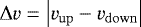 turns out to be the absolute variation range of the resulting outflow speed when one of the computational parameter is affected by an uncertainty of 30% with respect to its reference value. The panels of Fig. 11 show the Δ v maps for a ±30% variation of ne (a),
  (b), Te (c), and THI (d). We computed the Δv maps where vup and vdown are both higher than zero. We note that the images in the panels a and b are similar, since the Lyα resonant scattering process results to be equally depending on coronal electron density and chromospheric Lyα radiation. The mean values in the four Δv map panels (a–d) are 66.8, 66.8, 80.7, and 45.1 km s−1, respectively. This result provides a first order estimate of the H I outflow velocity uncertainty. Moreover, it indicates that the uncertainties of all the physical quantities characterising the emission of the resonantly scattered Lyα line can significantly affect the derivation of the solar wind speeds, with the coronal electron temperature uncertainty affecting it the most. It is worth remarking that further sources of uncertainty can be the assumptions of uniform Lyα radiation of the solar disk (see e.g. Auchère 2005) and isotropic H I temperature (see e.g. Dolei et al. 2016), as discussed above.
Figure 12 shows the Δv radial profiles as a function of the corresponding vref values at two different polar angles (PAs): above the solar north pole (PA = 0°) and along the radial direction in which we found the maximum value of vref (PA = 217°). The Δ v profiles in response to the variation of THI point out that the uncertainty of THI, which rougly affects the measurements of the solar wind velocity less than the other parameters (see Fig. 11), assumes a primary role at higher outflow speeds. We investigated the behaviour of the Δ v curves at all latitudes and found that the profiles related to the variation of THI assume values higher than those of the profiles related to the variation of the other physical parameters at H I outflow velocity about equal to 340 km s−1. In general, the shape of the Δ v curves in Fig. 12indicates that uncertainties of ne,  , and Te cause an uncertainty of the H I outflow velocity that monotonically decreases for increasing speed values vref. Conversely, the uncertainty of THI causes a Δ v that is a non-monotonic function of vref. In particular, we found Δv = 0 for vref about equal to 180–190 km s−1. It is worth noting that Δv = 0 implies vup = vdown, which means that a same dimming of the synthetic intensity of the resonantly scattered H I Lyα line was necessary to match the observed coronal UV intensity, even adopting two different THI values. The behaviour of the Lyα line intensity with the H I temperature was investigated by Dolei et al. (2015). These authors demonstrated that the Lyα resonant scattering process in the corona is favoured by a lower THI in regions of slow solar wind and by a higher THI in regions of fast solar wind, where coronal neutral hydrogen atoms with two different temperatures can contribute to a same scattered Lyα line radiation when outflowing with a same characteristic velocity. Finally, note also that the dashed curves in Fig. 12 present a profile similar to that of the derivative of the effective Doppler dimming coefficient (Fig. 1 shows the absolute value of the derivative), which is sensitive to the H I temperature (see Eq. (2)). In conclusion, beyond the analysis of the effective Doppler dimming coefficient, the parameter space exploration provides a further estimate of the range of uncertainty affecting the measurements of H I outflow velocity obtained through the Doppler dimming technique.
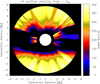 |
Fig. 10 H I outflow velocity map obtained by using the reference values of the physical quantities in the synthesis computation for the parameter space exploration, as described in the text. |
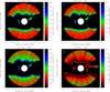 |
Fig. 11 Maps of speed absolute variation range in response to changing by a factor of ±30% the value of the parameters ne (panel a), |

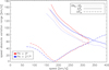 |
Fig. 12 Profiles of speed absolute variation range as a function of the vref values at 0° (red) and 217° (blue) of polar angle in response to changing by a factor of ±30% the value of the parameters ne (dotted lines), |

6 Summary and conclusions
We investigated the capability of mapping the solar wind H I outflow velocity in the inner heliosphere by using synergistic coronagraphic UV and VL observations, also in anticipation of the future science with the Metis instrument aboard the Solar Orbiter spacecraft, that will provide simultaneous coronagraphic imaging in broad-band polarised visible-light and narrow-band ultraviolet H I Lyα line.
We used observations acquired by space- and ground-based instruments, such as UVCS and LASCO aboard the SOHO spacecraft, and Mk3 installed at MLSO, and reconstructed UV and VL coronagraphic images similar to the images that will be obtained by the future Metis observations. We selected data over a time interval of 28 days in June 1997, covering a complete solar rotation, during the minimum phase between the solar magnetic activity cycles 22 and 23. We then synthesised the intensity of the resonantly scattered H I Lyα line by using electron densities derived from the VL images and physical quantities reported in the literature, and finally compared the result with the observed UV Lyα intensity. Exploiting the dependence of the coronal UV intensity of the Lyα line on the H I outflow speed, we applied the Doppler dimming technique to derive daily H I outflow velocity maps in the altitude range 1.5–4.0 R⊙.
Our investigation shows that the simultaneous availability of UV Lyα and VL polarised brightness images of the solar corona is suitable to get global maps of the H I outflow velocity in the inner heliosphere. Since there is close coupling between protons and neutral hydrogen atoms in this region of the solar corona, the H I outflow velocity maps also give information on the dynamics of protons. In general, they provide a clear picture of the distribution of the outflowing coronal plasma, both in heliocentric distance and in latitude. In particular, during the minimum phases of solar magnetic activity, they exhibit a clear boundary between the regions of fast (polar) and slow (equatorial) solar wind. In addition, the global maps can give the opportunity of investigating possible asymmetries in term of the outflow velocity between the two polar regions and provide useful information to bound the regions of the heliospheric current sheet and identify (single out) its roots in the corona.
The derivation of the solar wind H I outflow velocity maps from UV and VL images needs to adopt the values of physical quantities that are representative of the coronal environment, such as electron density and temperature, and H I temperature, and of the source of the UV radiation scattered by the coronal neutral hydrogen atoms, such as the profile of the chromospheric H I Lyα line radiation. Sometimes these quantities must be taken from the literature, because they cannot be directly determined from imaging data, as in the case of the data that will be provided by the Metis coronagraph. Therefore, we presented a critical discussion on the parameters adopted in the synthesis of the resonantly scattered Lyα line intensity and studied the dependence of the resulting outflow velocity on such quantities through a parameter space exploration. Our purpose was to investigate how the uncertainties affecting the adopted parameters influence the determination of the derived speeds. We found that all the sources of uncertainty can significantly affect the outflow velocity derivation; in particular, the coronal electron temperature uncertainty affects it the most, and the uncertainty of the H I temperature assumes a basic role at higher altitudes corresponding to higher outflow speeds.
Reasonable indications on the values of electron temperatures to use in the analysis of Metis data are expected from the measurements of the in situ instruments aboard Solar Orbiter, and, in particular, from the results of the ratios of the populations of different ion stages from the same element (see e.g. Ko et al. 1997; Cranmer et al. 1999). In addition, the values of the H I outflow velocity obtained in the equatorial regions below 4 R⊙ (see Fig. 7) support the assumption of a hydrostatic equilibrium regime, as proposed by Gibson et al. (1999). Hence, the electron temperatures can be inferred there by means of the electron densities derived from the VL polarised brightness images. We also note that the Gibson et al. (1999) method considers a single fluid plasma, therefore the calculated temperatures will be also assumed for the neutral hydrogen atoms. Regarding the H I temperature, suitable information can be provided by the extended database that was constructed by Dolei et al. (2016) from the analysis of a very large set of UVCS spectrometric data, complemented by the results of the temperature of protons obtained by the in situ instruments, although possible decoupling between protons and neutral hydrogen atoms at heliocentric distances around 10 R⊙ should be taken into account (see e.g. D’Amicis et al. 2007). The forthcoming space mission Parker Solar Probe, formerly Solar Probe Plus (Fox et al. 2016), should provide useful information on the temperature of protons just in the region where the decoupling is expected to begin, during its closest approaches to the sun. As for the chromospheric Lyα line radiation, Metis investigation will be supported by the images of the He II line emission at 30.4 nm of the entire solar disk that will be provided almost simultaneously by the Full Sun Imager (FSI) of the Extreme Ultraviolet Imager (EUI; Rochus et al. 2009) aboard Solar Orbiter, after correcting for the contribution of the nearby Si XI line. These images can be used to reconstruct maps of the chromospheric radiation of the H I Lyα line over the solar disk through the correlation of the intensity between the two spectral lines, as described by Auchère (2005). The chromospheric Lyα line maps serve, in turn, as reference signal for the application of the Doppler dimming technique, so reducing the margins of uncertainty. In addition, the anisotropy of the chromospheric radiation from the solar disk should be also taken into account in the derivation of the outflow velocity maps.
In conclusion, we have demonstrated that global maps of the solar wind H I outflow velocity in the inner heliosphere can be effectively obtained by the analysis of narrow-band imaging in Lyα, complemented by visible-light pB data. In particular, the Metis coronagraph aboard Solar Orbiter will provide precisely such data for the duration of the mission. The daily outflow velocity maps covering one whole month can be also used to construct coronal off-limb Carrington maps of the speeds at different heliocentric distances, in order to investigate the evolution of the outflowing plasma propagation and possible north-south pole asymmetries in the speed values during a complete solar rotation.
Movie
Movie of Sect. 4.2 Access Supplementary Material
Acknowledgements
The authors wish to thank the referee for his/her very helpful comments and suggestions, which led to a sounder version of the manuscript. The authors also acknowledge the partial support of the Italian Space Agency (ASI) to this work through contract ASI/INAF No. I/013/12/0.
References
- Andretta, V., Telloni, D., & Del Zanna, G. 2012, Sol. Phys., 279, 53 [NASA ADS] [CrossRef] [Google Scholar]
- Antonucci, E., Fineschi, S., Naletto, G., et al. 2012, SPIE, 8443, 9 [Google Scholar]
- Auchère, F., 2005, ApJ, 622, 737 [NASA ADS] [CrossRef] [Google Scholar]
- Auchère, F., Cook, J. W., Newmark, J. S., et al. 2005, ApJ, 625, 1036 [NASA ADS] [CrossRef] [Google Scholar]
- Bemporad, A. 2017, ApJ, 846, 86 [NASA ADS] [CrossRef] [Google Scholar]
- Bertaux, J.-L., Kyrölä, E., Quémerais, E., et al. 1995, Sol. Phys., 162, 403 [NASA ADS] [CrossRef] [Google Scholar]
- Bertaux, J.-L., Quémerais, E., Lallement, R., et al. 2000, Geophys. Res. Lett., 27, 1331 [NASA ADS] [CrossRef] [Google Scholar]
- Billings, D. E. 1966, A guide to the Solar Corona (New York: Academic Press) [Google Scholar]
- Brueckner, G. E., Howard, R. A., Koomen, M. J., et al. 1995, Sol. Phys., 162, 357 [NASA ADS] [CrossRef] [Google Scholar]
- Cranmer, S. R., Kohl, J. L., Noci, G., et al. 1999, ApJ, 511, 481 [NASA ADS] [CrossRef] [Google Scholar]
- D’Amicis, R., Orsini, S., Antonucci, E., et al. 2007, J. Geophys. Res., 112, 6110 [CrossRef] [Google Scholar]
- David, C., Gabriel, A.H., Bely-Dubau, F., et al. 1998, A&A, 336, 90 [NASA ADS] [Google Scholar]
- Del Zanna, G. 2008, A&A, 481, 49 [Google Scholar]
- Delaunay, B. 1934, Bulletin de l’Académie des Sciences de l’URSS, 6, 793 [Google Scholar]
- Dolei, S., Spadaro, D., & Ventura, R. 2015, A&A, 577, A34 [NASA ADS] [CrossRef] [EDP Sciences] [Google Scholar]
- Dolei, S., Spadaro, D., & Ventura, R. 2016, A&A, 592, A137 [NASA ADS] [CrossRef] [EDP Sciences] [Google Scholar]
- Domingo, V., Fleck, B., & Poland, A. I. 1995, Sol. Phys., 162, 1 [NASA ADS] [CrossRef] [Google Scholar]
- Fisher, R. R., Lee, R. H., MacQueen, R. M., & Poland, A. I. 1981, Appl. Opt., 20, 1094 [NASA ADS] [CrossRef] [Google Scholar]
- Fox, N. J., Velli, M. C., Bale, S. D., et al. 2016, Space Sci. Rev., 204, 7 [NASA ADS] [CrossRef] [Google Scholar]
- Frazin, R. A., Romoli, M., Kohl, J. L., et al. 2002, ISSIR, 2, 249 [NASA ADS] [Google Scholar]
- Frazin, R. A., Vásquez, A. M., Thompson, W. T., et al. 2012, Sol. Phys., 280, 273 [NASA ADS] [CrossRef] [Google Scholar]
- Gabriel, A. H. 1971, Sol. Phys., 21, 392 [NASA ADS] [CrossRef] [Google Scholar]
- Gibson, S. E., Fludra, A., Bagenal, F., et al. 1999, J. Geophys. Res., 104, 9691 [NASA ADS] [CrossRef] [Google Scholar]
- Harra, L. K., Sakao, T., Mandrini, C.H., et al. 2007, ApJ, 676, 147 [Google Scholar]
- Hayes, A. P., Vourlidas, A., & Howard, R. A. 2001, ApJ, 548, 1081 [NASA ADS] [CrossRef] [Google Scholar]
- Hess Webber, S. A., Karna, N., Pesnell, W. D., & Kirk, M. S. 2014, Sol. Phys., 289, 4047 [Google Scholar]
- Hyder, C. L., & Lytes, B. W. 1970, Sol. Phys., 14, 147 [NASA ADS] [Google Scholar]
- Ko, Y.-K., Fisk, L. A., Geiss, J., et al. 1997, Sol. Phys., 171, 345 [NASA ADS] [CrossRef] [Google Scholar]
- Kohl, J. L., Esser, R., Gardner, L. D., et al. 1995, Sol. Phys., 162, 313 [NASA ADS] [CrossRef] [Google Scholar]
- Kojima, M., Fujiki, K., Ohmi, T., et al. 2001, J. Geophys. Res., 106, 15677 [NASA ADS] [CrossRef] [Google Scholar]
- Lemaire, P., Emerich, C., Vial, J.-C., et al. 2002, in From Solar Min to Max: Half a Solar Cycle with SOHO, ed. A. Wilson, ESA SP, 508, 219 [Google Scholar]
- Low, B. C. 1990, ARA&A, 28, 491 [NASA ADS] [CrossRef] [Google Scholar]
- Lowder, C., Qiu, J., & Leamon, R. 2017, Sol. Phys., 292, 18 [NASA ADS] [CrossRef] [Google Scholar]
- Marsden, R. G., Wenzel, K.-P., & Smith, E. J. 1986, in The Sun and the Heliosphere in Three Dimensions, Proc. 19th ESLAB Symp., Astrophys. Space Sci. Lib., 123 (Dordrecht: D. Reidel Publishing Co.), 47 [Google Scholar]
- McComas, D. J., Barraclough, B. L., Funsten, H. O., et al. 2000, J. Geophys. Res., 105, 10419 [NASA ADS] [CrossRef] [Google Scholar]
- Müller, D., Marsden, R. G., St. Cyr, O. C. & Gilbert, H. R., 2013, Sol. Phys., 285, 25 [NASA ADS] [CrossRef] [Google Scholar]
- Noci, G., & Maccari, L. 1999, A&A, 341, 275 [NASA ADS] [Google Scholar]
- Noci, G., Kohl, J. L., & Withbroe, G. L. 1987, ApJ, 315, 706 [NASA ADS] [CrossRef] [Google Scholar]
- Priest, E. R. 1987, Solar Magneto-Hydrodynamics, ed. Publishing Company (Dordrecht: Reidel) [Google Scholar]
- Raymond, J. C., Kohl, J. L., Noci, G., et al. 1997, Sol. Phys., 175, 645 [NASA ADS] [CrossRef] [Google Scholar]
- Reber, C. A. 1990, EOS, 71, 1867 [NASA ADS] [CrossRef] [Google Scholar]
- Roberts, D. A., & Goldstein, M. L. 1998, Geophys. Res. Lett., 25, 595 [NASA ADS] [CrossRef] [Google Scholar]
- Rochus, P., Halain, J.-P., Renotte, E., et al. 2009, 60th Int. Astron. Congress, A3, 4 [Google Scholar]
- Rottman, G. J., & Woods, T. N. 1994, SPIE, 2266, 317 [NASA ADS] [Google Scholar]
- Svalgaard, L., & Kamide, Y. 2013, ApJ, 763, 23 [NASA ADS] [CrossRef] [Google Scholar]
- Spadaro, D., & Ventura, R. 1994, A&A, 289, 279 [NASA ADS] [Google Scholar]
- Spadaro, D., Susino, R., Ventura, R., Vourlidas, A., & Landi, E. 2007, A&A, 475, 707 [NASA ADS] [CrossRef] [EDP Sciences] [Google Scholar]
- Susino, R., Ventura, R., Spadaro, D., Vourlidas, A., & Landi, E. 2008, A&A, 488, 303 [NASA ADS] [CrossRef] [EDP Sciences] [Google Scholar]
- Telloni, D., Antonucci, E., & Dodero, M. A. 2007, A&A, 476, 1341 [NASA ADS] [CrossRef] [EDP Sciences] [Google Scholar]
- Van De Hulst, H. C. 1950, Bull. Astron. Inst. Netherland, 410, 135 [Google Scholar]
- Vasquez, A. M., Van Ballegooijen, A. A., & Raymond, J. C. 2003, ApJ, 598, 1361 [NASA ADS] [CrossRef] [Google Scholar]
- Withbroe, G. L., Kohl, J. L., Weiser, H., & Munro, R. H. 1982, Space Sci. Rev., 33, 17 [NASA ADS] [CrossRef] [Google Scholar]
All Tables
All Figures
|
Fig. 1 Effective Doppler dimming coefficient of the resonantly scattered H I Lyα line (solid lines) and absolute value of its derivative with respect to the outflow speed (dashed lines), calculated at the heliocentric distance r = 2.5 R⊙, on the plane of the sky of the observer, for a polar coronal hole (CH) with THI = 2.2 MK averaged along the LOS (red lines), and r = 4.0 R⊙ for an equatorial streamer (STR) with THI = 1.6 MK averaged along the LOS (green lines). |
| In the text | |
|
Fig. 2 Left panels: UV H I Lyα line intensityon the 1st June 1997, in units of photons cm−2 s−1 sr−1, as measured by the UVCS daily synoptic observation (top) and reconstructed between 1.5 and 6.0 R⊙ (bottom). Right panels: VL polarised brightness on the 1st June 1997, in units of Mean Solar Brightness (MSB), asmeasured by the LASCO C2 and Mk3 coronagraphs (top) and reconstructed between 1.5 and 6.0 R⊙ (bottom). |
| In the text | |
|
Fig. 3 Coronal electron density profiles in equatorial (green solid line) and polar (red solid line) regions obtained by means of the Van De Hulst inversion technique. The dotted areas represent the range of density uncertainty corresponding to a ±10% variation of the polarised brightness profiles. |
| In the text | |
|
Fig. 4 Adopted normalised chromospheric H I Lyα line profile. |
| In the text | |
|
Fig. 5 Coronal electron temperature profiles adopted for equatorial (dotted line) and polar (dashed line) regions. The shaded area corresponds to the sequence of Te profiles usedfor the mid-latitude regions. |
| In the text | |
|
Fig. 6 Top panel: map of the THI values at solar minimum obtained by Dolei et al. (2016) from the analysis of the Lyα line width. Bottom panel: adopted coronal H I temperature map. |
| In the text | |
|
Fig. 9 Coronal off-limb Carrington maps of H I outflow velocity at 2.5 (top) and 3.5 R⊙ (bottom). The void areas correspond to the gaps in the UVCS synoptic data. |
| In the text | |
|
Fig. 7 Top panels: H I outflow velocity maps on the 1st (left) and 14th (right) June 1997. Bottom panels: H I outflow velocity radial profiles in the equatorial and polar regions on the 1st (left) and 14th (right) June 1997. The dottedareas represent the range of speed uncertainty as a result of an uncertainty of the reconstructed UV Lyα line intensity by 3%, according to the variation rate of the effective Doppler dimming coefficient. |
| In the text | |
|
Fig. 8 H Ioutflow velocities over the investigated time interval: equatorial radial profiles (top); polar radial profiles (middle); latitudinal profiles (bottom) at 2.5 (cyan lines) and 3.5 R⊙ (purple lines). In particular, the equatorial radial profiles decreasing with height for lower altitudes correspond to speeds in the wind streams, such as those shown in the top panels of Fig. 7 (see discussion in the text). |
| In the text | |
|
Fig. 10 H I outflow velocity map obtained by using the reference values of the physical quantities in the synthesis computation for the parameter space exploration, as described in the text. |
| In the text | |
|
Fig. 11 Maps of speed absolute variation range in response to changing by a factor of ±30% the value of the parameters ne (panel a), |
| In the text | |
|
Fig. 12 Profiles of speed absolute variation range as a function of the vref values at 0° (red) and 217° (blue) of polar angle in response to changing by a factor of ±30% the value of the parameters ne (dotted lines), |
| In the text | |
Current usage metrics show cumulative count of Article Views (full-text article views including HTML views, PDF and ePub downloads, according to the available data) and Abstracts Views on Vision4Press platform.
Data correspond to usage on the plateform after 2015. The current usage metrics is available 48-96 hours after online publication and is updated daily on week days.
Initial download of the metrics may take a while.