| Issue |
A&A
Volume 611, March 2018
|
|
|---|---|---|
| Article Number | A44 | |
| Number of page(s) | 11 | |
| Section | Extragalactic astronomy | |
| DOI | https://doi.org/10.1051/0004-6361/201731987 | |
| Published online | 21 March 2018 | |
Broadband study of blazar 1ES 1959+650 during flaring state in 2016
1
Department of High Energy Physics, Tata Institute of Fundamental Research,
Mumbai
400005, India
e-mail: This email address is being protected from spambots. You need JavaScript enabled to view it.
2
Universität Würzburg,
97074
Würzburg, Germany
3
Department of Physics, University of Mumbai, Santacruz (East),
Mumbai
400098, India
Received:
23
September
2017
Accepted:
13
November
2017
Abstract
Aims. The nearby TeV blazar 1ES 1959+650 (z = 0.047) was reported to be in flaring state during June–July 2016 by Fermi-LAT, FACT, MAGIC and VERITAS collaborations. We studied the spectral energy distributions (SEDs) in different states of the flare during MJD 57530–57589 using simultaneous multiwaveband data with the aim of understanding the possible broadband emission scenario during the flare.
Methods. The UV-optical and X-ray data from UVOT and XRT respectively on board Swift and high energy γ-ray data from Fermi-LAT were used to generate multiwaveband lightcurves as well as to obtain high flux states and quiescent state SEDs. The correlation and lag between different energy bands was quantified using discrete correlation function. The synchrotron self-Compton (SSC) model was used to reproduce the observed SEDs during flaring and quiescent states of the source.
Results. A good correlation is seen between X-ray and high energy γ-ray fluxes. The spectral hardening with increase in the flux is seen in X-ray band. The power law index vs. flux plot in γ-ray band indicates the different emission regions for 0.1–3 GeV and 3–300 GeV energy photons. Two zone SSC model satisfactorily fits the observed broadband SEDs. The inner zone is mainly responsible for producing synchrotron peak and high energy γ-ray part of the SED in all states. The second zone is mainly required to produce less variable optical-UV and low energy γ-ray emission.
Conclusions. Conventional single zone SSC model does not satisfactorily explain broadband emission during observation period considered. There is an indication of two emission zones in the jet which are responsible for producing broadband emission from optical to high energy γ-rays.
Key words: radiation mechanisms: non-thermal / BL Lacertae objects: individual: 1ES 1959+650 / gamma rays: general / X-rays: galaxies
© ESO 2018
1 Introduction
Blazars are a subclass of active galactic nuclei having relativistic jets pointing close to our line of sight (Urry & Padovani 1995). Jets emit highly variable non-thermal radiation spanning wide band of frequencies from radio to γ-rays. Blazars include two types of objects, BL Lacertae (BL Lac) characterized by featureless optical spectra and flat spectrum radio quasars which show prominent emission lines.
The spectral energy distributions (SEDs) of these objects show characteristic two hump structure. The first low frequency hump is attributed to the synchrotron radiation from relativistic electrons, while second high frequency hump is understood as possibly corresponding to inverse Compton scattering of these synchrotron photons (synchrotron self-Compton, SSC) or external photons (external Compton, EC) by the same population of electrons. Alternative explanation for origin of the second hump is given in terms of hadronic models including neutral pion decay, proton synchrotron (Mannheim 1998), etc. A comprehensive review of these mechanisms is given by Böttcher (2007).
Depending on the position of synchrotron peak in SED, BL Lacs are further divided into three classes (Padovani & Giommi 1995). Low frequency BL Lac objects exhibit synchrotron peak in IR-Optical band, intermediate frequency BL Lac objects have their synchrotron peak at optical-UV frequencies and high frequency BL Lac (HBL) objects show a synchrotron peak in the UV to X-ray band.
The HBL object, 1ES 1959+650 (z = 0.047) was first detected in radio band with NRAO Green Bank 91 m telescope (Becker et al. 1991; Gregory & Condon 1991) and later in X-ray (Schachter et al. 1993) using Imaging Proportional counter on board Einstein Observatory. TeV emission from this source was first observed by the Utah Seven Telescope Array collaboration with total significance of 3.9σ above 600 GeV (Nishiyama 1999). The source was later observed during 2002 May 16 to July 8, with strong detection significance of >20σ by Whipple 10 m telescope (Holder et al. 2003). Since then several flaring episodes have been shown at VHE (>100 GeV) γ-ray energies. The most noticeable episode was in 2002 and showed enhanced TeV emission without any contemporaneous X-ray flare (Aharonian et al. 2003; Krawczynski et al. 2004; Daniel et al. 2005; Reimer et al. 2005). In 2004, the source was observed in low state by MAGIC collaboration with a flux of about 20% of the Crab and at ~8σ significance level above ~180 GeV (Albert et al. 2006). Broadband variability of the source was studied in 2012 using strictly simultaneous observations from VERITAS and Swift and reflected emission scenario was used to explain the variability (Aliu et al. 2014). The preliminary analysis of data from Fermi-LAT and various ground based Cherenkov experiments such as FACT, MAGIC, VERITAS as reported by Buson et al. (2016), indicated flaring activity in the source from 27 April 2016 onwards.
In the present paper, we have examined the multiwaveband emission from this source over 800 days during MJD 57000 to 57800 (9 December 2014 to 16 February 2017) and studied the broadband variability of this source for the period from MJD 57530 to 57589 (22 May 2016 to 20 July 2016) during which it showed increased flux in X-ray, Fermi-LAT (100 MeV–300 GeV) and TeV bands. To have good statistics in LAT energy band (0.1–300 GeV), we chose six periods of 10 days each to sample the complete flare and investigated its emission mechanism in different states during the flare using SSC model. We also studied the SED corresponding to a period of 10 days during which the source was in a low state. The paper is organized as follows. In Sect. 2 various data sets and analysis methods are described. In Sect. 3timing and spectral studies are elaborated. The SED modelling isoutlined in Sect. 4 followed by discussion and conclusions in Sect. 5.
2 Multiwaveband observations and analysis
We have studied the multiwaveband data from radio to γ-rays spanning the period of more than two years from 9 December 2014 (MJD 57000) to 16 February 2017 (MJD 57800). We analysed UV-optical data from Swift-UVOT, X-ray data from Swift-XRT and high energy γ-ray data from Fermi-LAT. We also used publicly available data from OVRO, SPOL, MAXI and Swift-BAT. Details of these data sets and analysis procedure are given below.
2.1 High energy γ-ray observations
High energy γ-ray data covering the energy range of 100 MeV–300 GeV was obtained from Large Area Telescope (LAT) on board Fermi spacecraft (Atwood et al. 2009). Data were analysed using Science Tools version v10r0p5. The user contributed Enrico package (Sanchez & Deil 2013) was used. The events were extracted from the circular region of interest (ROI) of 20° centered on the source. Zenith angle cut of 90° was applied to filter the background γ-rays from Earth’s limb. To select good time intervals, a filter with “(DATA_QUAL>0)&&(LAT_CONFIG==1)” was used. The spectral analysis was carried out using the isotropic emission model (iso_P8R2_SOURCE_V6_v06.txt) and galactic diffuse emission component model (gll_iem_v06.fit) with the post launch instrument response function (P8R2_SOURCE_V6) and using unbinned likelihood analysis. The sources lying within ROI of 15° radius around the 1ES 1959+650 from the 3FGL catalogue were included in the model XML file. In likelihood fit, both spectral and normalization parameters of the sources within 5° radius around the source were left free to vary while keeping parameters for all other sources fixed at their catalogue value. There are 72 point sources and one extended source in the model file. The parameters of the extended source were also kept free in a maximum likelihood analysis. The source spectrum was modelled with a power law. The lightcurves were generated with 10-day binning in the energy ranges 0.1–3 GeVand 3–300 GeV.
2.2 X-ray observations
Publicly available hard X-ray data from the Burst Alert Telescope (BAT) on board Swift are used1. These are daily average count rates over the energy range of 15–50 keV. Soft X-ray data covering the energy range of 2–20 keV from the Monitor of All sky X-ray Images (MAXI) on board the International Space Station (ISS; Matsuoka et al. (2009)) are obtained from MAXI website2. These are daily average flux values.
Soft X-ray data covering the energy range of 0.3–8 keV from X-ray telescope (XRT) on board Swift have also been used (Burrows et al. 2005). The data were analysed using XRT Data Analysis Software (XRTDAS) distributed within the HEASOFT package (v6.19). The xrtpipeline-0.13.2 tool was used to generate the cleaned event files. Data from 34 observations during the period 22 April–20 July 2016 corresponding to the flare region were analysed. The source and background data were extracted from the circular 20-pixel radius region around the source and a 40-pixel radius region away from the source respectively. The spectral data were combined into six groups of 10 days each as shown in Fig. 1 and rebinned with minimum 20 photons per bin. Six spectra were fitted with an absorbed power law model as well as with a logparabola model. The spectral form of the logparabola model is given by
 (1)
where α is the spectral index and Ep is the point of maximum curvature given by
(1)
where α is the spectral index and Ep is the point of maximum curvature given by
 (2)
(2)
While fitting the spectrum, Eb is fixed at 1 keV. To correct for interstellar absorption of soft X-rays along the line of sight, neutral hydrogen column density (NH ) is fixed at 1.0 ×1021 cm−2 (Kalberla et al. 2005). Swift XRT light curve spanning two years’ data, over the energy range 0.3–10 keV is shown in Fig. 1. This is the publicly available Swift-XRT lightcurve obtained from the Swift website3 .
2.3 UV, optical and radio observations
We have analysed Swift-UVOT (Roming et al. 2005) data for a period of two years. Data are available in six different filters covering optical and UV band, viz. V , B, U, UVW1, UVM2 and UVW2.For each filter, images were added using the uvotimsum tool. The flux and magnitude values were obtained using tool uvotsource. For the V , B, and U filters, source counts were extracted from a circular region with radius 5” around the source location, whereas for the UVW1, UVM2, andUVW2 filters, a region with radius 10” was used. The Galactic extinction correction (Schlegel et al. 1998) of EB −V = 0.177 mag was applied to the observed magnitude. Observed magnitudes were then converted into flux using zero point magnitudes (Poole et al. 2008). Host galaxy contributions (Tagliaferri et al. 2008) of 1.1 mJy, 0.4 mJy, and 0.1 mJy were subtracted for V , B, and U filter respectively. No correction was applied at UV frequencies as host galaxy contribution is negligible atthese frequencies. Figure 1 shows lightcurves from optical U and ultravilolet M2 filters. Other UVOT bands show similar trend, hence only two bands are shown to avoid cluttering.
The source 1ES 1959+650 is being monitored with the SPOL CCD Imaging/Spectropolarimeter at steward observatory at the University of Arizona (Smith et al. 2009) regularly as a part of the Fermi multiwavelength support programme. The publicly available optical R-band and V-band photometric and linear polarization data were obtained from the SPOL website4 . The R-band fluxes are corrected for host galaxy contribution which is 0.84 mJy (Nilsson et al. 2007). From the available data the degree of linear polarization and polarization angles were found to vary between 0.37% to 3.98% and 107° to 173° respectively.
1ES 1959+650 is also observed regularly in radio as a part of Fermi monitoring programme by Owens Valley Radio Observatory (OVRO; Richards et al. 2011). The publicly available data at 15 GHz were used as the lightcurve from OVRO website5 .
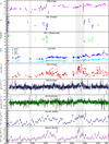 |
Fig. 1 Two years light curves of 1ES 1959+650 from MJD 57000 to 57800. Panel 1: radio flux density at 15 GHz in Jy. Panel 2: degree of polarization from CCD-SPOL observations. Panel 3: polarization angle from CCD-SPOL observations. Panel 4: UVOT-U, UVOT-W2 band and CCD-SPOL-R band fluxes in mJy (corrected for host galaxy contribution). Panel 5: Swift-XRT count rate in counts/s. Panel 6: MAXI flux in photons cm−2 s−1 (daily average). Panel 7: Swift-BAT flux in counts cm−2 s−1 (daily average). Panel 8: Fermi-LAT 0.1–3 GeV flux in photons cm−2 s−1 (10 days average). Panel 9: Fermi-LAT 3–300 GeV flux in photons cm−2 s−1 (10 days average). SEDs are computed for the periods marked by dotted lines. |
3 Results
In this section we present results from multiwaveband temporal and spectralstudies of 1ES 1959+650 collected over a two-year period from MJD 57000 to 57800.
3.1 Multiwaveband temporal studies
Figure 1 shows the lightcurve of 1ES 1959+650 for the period MJD 57000 to 57800. Panels corresponding to various wavebands have been arranged in increasing order of frequency from top to bottom, starting with radio lightcurve from OVRO in the topmost panel to high energy γ-rays from Fermi-LAT in the bottom-most panel. Fermi-LAT flux values over the energy ranges 0.1–3 GeV and 3–300 GeV shown in last two panels, are averaged over bins of 10 days. Data from Swift-BAT and MAXI are averaged over a day, whereas Swift-XRT and Swift-UVOT data points correspond to individual observationswith typical duration of minutes or hours. SPOL and OVRO have an integration time of a few seconds. The source exhibited the flare in 2016 during MJD 57530–57589. This flare is clearly seen in the figure particularly in X-ray and γ-ray bands. We studied correlated variability in various wavebands. In this workwe have concentrated on detailed studies during the flaring episode around MJD 57530–57589 (22 May–20 July 2016). This episode is divided into six periods of 10 days. Quiescent state data during MJD 57177–57186 (4–13 June 2015) is compared with this flare.
3.1.1 Variability
We have studied the variability of lightcurves in various wavebands on various timescales. Variability is estimated in terms of fractional variability amplitude, Fvar parameter (Vaughan et al. 2003; Chitnis et al. 2009). This parameter estimates variability intrinsic to the source and is given by
 (3)
where S2 is the sample variance,
(3)
where S2 is the sample variance,  the mean square error and
  the unweighted sample mean. The error on the Fvar is given by
 (4)
(4)
Variability strength is estimated on timescales of 10 and 20 days in various wavebands in present work. Results are given in Table 1 and plotted in Fig. 2 for 10-day binning. The large error bar on BAT is due to the poor sensitivity of the instrument. Variability seems to increase with frequency from radio to X-rays and decrease in high energy γ-rays compared to hard X-rays. A similar trend was seen in Mkn 421 (Sinha et al. 2016).
Fractional variability strength in various wavebands.
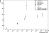 |
Fig. 2 Fractional variability for the 10-day binned lightcurve. |
3.1.2 Correlations
The correlations between various lightcurves are quantified over the entire observation period (MJD 57000 to 57800) using a discrete correlation function (DCF; Edelson & Krolik 1988). For two discrete data sets ai and bj , the unbinned discrete correlation is defined as
 (5)
for all measured pairs (ai ,bj ) having pairwise lag Δtij = tj − ti. Standard deviations σa and σb are for the two data trains and ea, and eb are the measurement errors associated with them. We then obtain DCF by averaging M pairs for which (τ −Δτ∕2) ≤Δtij < (τ + Δτ∕2),
(5)
for all measured pairs (ai ,bj ) having pairwise lag Δtij = tj − ti. Standard deviations σa and σb are for the two data trains and ea, and eb are the measurement errors associated with them. We then obtain DCF by averaging M pairs for which (τ −Δτ∕2) ≤Δtij < (τ + Δτ∕2),
 (6)
(6)
The error on DCF is given by
![Mathematical equation: \begin{equation}\label{eq7} \sigma_{DCF}(\tau) = \frac{1}{M-1} \left\{ \sum_{}^{} [ UDCF_{ij} - DCF(\tau) ] \right\}^{1/2} .\end{equation}](/articles/aa/full_html/2018/03/aa31987-17/aa31987-17-eq9.png) (7)
(7)
Each data set is linearly de-trended (Welsh 1999) before using above function. The correlation coefficients along with lags between the lightcurves are listed in Table 2 and their plots are shown in Fig. 3. Values of correlation coefficients given in the table and figure are estimated for 3-day binning in lag to improve the statistics, except for the case of 0.1–3 GeV to 3–300 GeV where a bin size of 10 days is used. These values are consistent with 1-day binning of the lag in all cases. It can be seen that there is a strong correlation between optical (V band) and UV (M2 band) at zero lag. X-ray data shows good correlation with low and high energy γ-rays with no visible lag. Correlation is better with higher energy γ-rays. Low and high energy γ-rays are also correlated. A mild correlation is seen between optical (V band) and γ-rays with a lag of about 38–90 days. Similar lag is seen between radio and γ-rays. On the other hand, the correlation between the optical and X-ray bands is rather weak. This indicates that X-rays and higher energy γ-rays may have similar origin. Whereas the optical-UV band emission may have a different origin. The study of long-term data (2005–2014) carried out by Kapanadze et al. (2016) showed that the source displayed slow variation in the optical R band and exhibited an optical flare lasting several months to years. They also report a relatively weak correlation between the XRT and UVOT bands.
Maximum DCF between various wavebands.
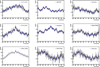 |
Fig. 3 Discrete correlation function vs. time lag between various energy bands. |
3.1.3 Lognormality
Lognormality, that is, the log-normal distribution of flux and the linear rms-flux relation, has been detected in several X-ray binaries (Uttley & McHardy 2001; Scaringi et al. 2012). It has also been detected in blazars including BL Lac (detected in X-ray regime, Giebels & Degrange 2009), in multiple wavebands in PKS 2155-304 (Chevalier et al. 2015), Mkn 421 (Sinha et al. 2016), 1ES 1011+496 (Sinha et al. 2017), and PKS 1510-089 (Kushwaha et al. 2016) amongst others. Flux distributions for 1ES 1959+650 covering two years’ data for various wavebands from radio to γ-ray are shown in Fig. 4. Data are fitted with Gaussian as well as lognormal distributions and these fits are shown. Reduced χ2 values for both the distributions are listed in Table 3. Reduced χ2 is lower for the lognormal than the Gaussian fit in all cases, except for that of 0.1–3 GeV Fermi-LAT. In order to check the significance of this reduction in χ2 , the F-statistic was used. Assuming no significant difference in variances from these two models (the null hypothesis), F-values were calculated (Fcalculated). These were compared with F-values for 95% confidence level (F95%), for νg and νl degrees of freedom (d.o.f.; corresponding to Gaussian and lognormal fits respectively). These values are listed in Table 3 for each waveband. It can be seen that Fcalculated are less than F95% in all cases, which means that we can not reject the null hypothesis. In other words, even though lognormal gives lower χ2 and better fit, Gaussian behaviour can not be ruled out at 95% confidence because of the low number of d.o.f. Figure 5 shows the plot of excess variance  as a function of flux for various X-ray wavebands, binned over a period of 10 days. The excess variances were calculated for those bins that have at least five flux points and are plotted against mean flux. We do not see the very clear linear trend in these plots that was seen in the case of Mkn 421 by Sinha et al. (2016).
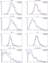 |
Fig. 4 Gaussian and lognormal fit to flux distribution in various energy bands. The binning used is the same as in Fig. 1 except for MAXI and BAT where 10-day binning is used. |
Goodness of fit for flux distributions in various energy bands.
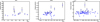 |
Fig. 5 Excess variance vs. mean flux in different X-ray energy bands: the data are binned into 10-day bins and excess variance is computed only for those bins which have at least five flux measurements. |
3.2 Spectral studies
We studied X-ray spectra using Swift-XRT data for the flare state during MJD 57530–57589. This flare was divided into six states, each spanning a 10-day period. These states are indicated in Fig. 1. We also studied the X-ray spectrum in the interval MJD 57177–57187 which corresponds to the quiescent state of the source. These seven average spectra for each bin were fitted with a power law with line of sight absorption, over the energy range of 0.3–8 keV. Spectra were also fitted with logparabola model with line of sight absorption. Best fit parameters for both the models are given in Table 4. Logparabola seems to fit data better than power law, as seen from improvement in values of reduced χ2.
We also analysed X-ray spectra from individual observations of XRT during the flare. Figure 6 shows the plot of flux in 0.3–8 keV range as a function of X-ray photon index for both the power law and logparabola models. The X-ray spectrum seems to harden with the increase in flux. Similar behaviour from this source is also reported by Gutierrez et al. (2006). However no such correlation was found when the source was observed in a low state during the period 2007–2011 (Aliu et al. 2013). Spectral hardening with an increase in flux is seen in several other blazars including Mkn 421 (Sinha et al. 2016); Mkn 501 (Krawczynski et al. 2000).
We also investigated spectral parameters in the γ-ray band using Fermi-LAT data, dividing it into two energy ranges, 0.1–3 GeV and 3–300 GeV. Spectra binned over 10 days were fitted with a power law. Variation of flux with a power law index for both low and high energy bands is shown in Fig. 7. While lower energy band shows increase in the flux with an increase in the photon index, no such trend is seen at higher energies. Similar behaviour at γ-ray energies was seen for Mkn 501 (Shukla et al. 2015). Such a trend might be due to different emission regions for low and high energy γ-rays. Figure 8 shows the hardness ratio, defined as the ratio of 3–300 GeV to 0.1–3 GeV flux, as a function of 0.1–3 GeV flux. This also indicates that for the period of 800 days the spectrum becomes softer at higher flux.
Spectral fitting parameters for 10-day binned Swift-XRT data.
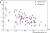 |
Fig. 6 Power law index vs. X-ray flux (the correlation coefficient is −0.72; red) and logparabola index vs. X-ray flux (the correlation coefficient is −0.61; blue). |
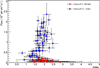 |
Fig. 7 Power law index vs. LAT flux. The correlation coefficient for the 0.1–3 GeV band is 0.60. |
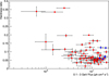 |
Fig. 8 Hardness ratio in Fermi band vs. 0.1–3 GeV flux, Points corresponding to the flare are shown in blue. |
4 Evolution and modelling of the SED
We have studied the evolution of the SED during flare. For this purpose, multiwaveband SEDs were generated for six flux states in the flare as well as for one quiescent state. First we tried to model these SEDs using simple single zone SSC model using the code developed by Krawczynski et al. (2004). This model assumes the emission zone to be a blob of radius R traveling down the jet with bulk Lorentz factor Γ towards the observer at an angle of θ. The emission zone is filled with non-thermal electron distribution and a randomly orientated magnetic field. The electron population can be described by a broken power law, having low and high energy indices p1 and p2. The radius R of the emission region can be constrained by observed flux-doubling timescale (tvar) using the relation,
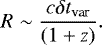 (8)
(8)
The six flux states during different epochs of the flare are denoted by F1, F2, F3, F4, F5, and F6 while quiescent state is denoted by Q. The SEDs were modelled with jet parameters θ and Γ to be 3° and 9.4 respectively which corresponds to a Doppler factor of ~15. The value ofthe Doppler factor is consistent with the reported value (Krawczynski et al. 2004; Gutierrez et al. 2006). Blob radius 7.84 ×1016 cm was assumed. While modelling θ was kept fixed at three degrees and it is also assumed that the emitting region has the same cross section as the jet.
We findthat due to sharp curvature of SEDs in X-ray region, we always underpredict the optical-UV flux with a one-zone SSC model. Also, except for the F2 state, the one zone SSC model does not fit γ-ray flux below ~3 GeV. Hence we made an attempt to explain the observed SEDs with a two-zone SSC model in which the resultant emission is the sum of the emissions from two comoving blobs of different sizes. We assumed thesize of the second (outer) blob to correspond to tvar ~ 10 days and to have the same Doppler factor as that of the inner blob. The cross plot of the flux-power law index in the 0.1–3 GeV and 3–300 GeV bands suggests different emission regions for these energy bands (Fig. 7). It is reported in the long term (2005–2014) multiwavelength cross-correlation study that one zone SSC scenario was not always suitable to explain the emission from this source (Kapanadze et al. 2016).
The fits for all six high states are shown in Fig. 9 and one quiescent state is shown in Fig. 10. Figure 11 shows the variation of inner blob emission as the flare evolves. The SSC model parameters for two zones are listed in Table 5. Apart from the conventional single-zone SSC model, EC, lepto-hadronic model, and two independent SSC models have been tried for fitting SEDs in the past (Backes et al. 2012). Authors report that a two-zone SSC model described the observed SED reasonably well for this source. The two-zone SSC model was also used to reproduce the observed SED during the 2011 observation of Mkn 501 (Shukla et al. 2015, 2016).
In a homogeneous leptonic model, one expects a break in electron energy distribution (EED) where Lorentz factor is given by
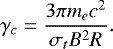 (9)
(9)
At this γc, the escape time from the source equals the synchrotron cooling time (Abdo et al. 2011; Graff et al. 2008). Figure 12 shows variation of fitted B with γbr for flare states F1–F6. The theoretical curve based on Eq. (9) assuming R = 7.84 × 1016 cm is shown for the inner blob. As per Eq. (9), we find that observed B is up to ~45% lower than expected (Fig. 12). This means that we observe a break in electron spectrum at lower energies than that expected in the case of similar escape and cooling timescales.
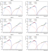 |
Fig. 9 SEDs fitted with two zone SSC model for six states during flare. |
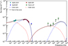 |
Fig. 10 Quiescent state SED fitted with the two-zone SSC model. |
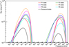 |
Fig. 11 Variation of inner zone of SSC emission during six flare and one quiescent states. |
SSC model parameters for flare and quiescent states for two zones that have Doppler factor (δ) ~ 15, θ = 3, Rinner = 7.84 × 1016 cm (tvar ~ 2 days) and Router = 3.92 × 1017 cm (tvar ~ 10 days).
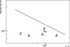 |
Fig. 12 Temporal evolution of model parameter B with γbr for inner zone. The theoretical curve is shown by the black continuous line as per Eq. (9). |
5 Discussion and conclusions
The lognormal fit to the flux distribution of two years’ data gives improved reduced χ2 as compared to a Gaussian fit. However we do not see this difference between models to be significant based on the F-test. This could be due to the smaller size of the data set. Since the tail is seen in the flux distribution, possibly a longer data set may be shown to be significantly preferable to the lognormal fit. Several authors have seen lognormal behaviour of flux distribution in X-ray binaries and BL-Lac sources. The lognormal flux behaviour in BL-Lac is generally considered as an indication of the accretion disc variability’s imprint onto the jet (McHardy 2008). In the present data set, we do not see convincing lognormality. A longer data set may lead to a conclusive result.
The temporal analysis of two years’ data on 1ES 1959+650 shows that the source did not exhibit significant variation in the optical band. However, the source showed significant flux variation in the X-ray and γ-ray bands. The DCFs were computed to quantify the correlations and lags between measurements from various instruments covering different energy bands over two years. A significant correlation is seen between fluxes of X-ray, and both high and low energy γ-rays. No significant correlation of optical-UV fluxes with other energy bands was seen. This could be due to different emission region of optical-UV photons and these photons are up-scattered to low energy γ-rays, which might be observed by Fermi-LAT.
We found the X-ray spectrum to be curved during most of the observations and hence the logparabola fit to the X-ray spectrum is found to be better than conventional power law fit. The logparabola fit to the X-ray data also suggests that particle acceleration should be stochastic in nature. The spectral evolution was found to be “harder when brighter” in the X-ray during the observation period of approximately two months covering the flare. However, “softer when brighter” behaviour was also seen in γ-rays (Fig. 8) when the source was not very active.
We found a significant change in electron density across the flare in both inner and outer regions by modelling of SEDs. However a maximum ~20% change is observed in the magnetic field. Either injection of new particles or re-acceleration of particles might have increased electron energy density in the inner zone. This enhanced electron energy density might be responsible for the high state and flaring activity of the source. Also, similar magnetic field in outer blob might be due to re-amplification of magnetic filed by passing shock wave. A narrow EED and spectral hardening are found in the electron spectrum during the flaring period from the inner blob. The narrow EED can be reconciled as a stochastic acceleration process via a Fermi II order acceleration scenario, where randomly moving Alfvén waves may accelerate particles in turbulent medium.
The observed break in the particle spectrum found by SED modelling isat much lower energies than the expected from the canonical jet model (Eq. (9)) as seen in Fig. 12. This observed break in the particle spectrum might be an outcome of effective inverse Compton cooling and this break appears at the Lorentz factor where inverse Compton cooling equals adiabatic losses. In our SED modelling, inverse Compton losses dominate synchrotron losses. Similar behaviour is observed in Mkn 501 (Acciari et al. 2011). The magnetic field and electron energy density in the inner region was found to be an order of magnitude higher than in the outer region. Moreover, electron spectra were found to be much softer here than in the inner blob . The particle spectra in the outer blob might be the outcome of shock acceleration where particles are cooled through synchrotron and IC losses.
With an increase in the flux, the synchrotron peak is found to shift to the right and vice-versa. This is the “bluer when brighter” behaviour of the source during this period. Similar behaviour is reported by Tagliaferri et al. (2008). Among the six states, the F2, F3, and F4 states sampled the peak of the flare. During the F3 and F4 states the high energy γ-ray flux is comparable while there is a significant increase in the X-ray flux as the state evolved from F3 to F4. It was then followed by the decrease in the flux in both synchrotron and IC region as the flare decays in the F5 and F6 states.
We are able to reproduce SEDs satisfactorily with a broken power law electron distribution with (p2 − p1) ~ 1, for both inner and outer regions. This corresponds to a spectral index change of Δα = 0.5 for synchrotron emission, which is expected in the case of a canonical cooling break in the homogeneous model. We could reproduce all the flaring states and one quiescent state with a Doppler factor of ~15 for both comoving plasma blobs. The higher γmin seen in the inner blob compared to the outer blob suggests the narrower EED of the inner blob. The narrow EED is responsible for producing the hard spectrum (Tavecchio et al. 2009; Katarzyński et al. 2006; Lefa et al. 2011). During flaring activity the inner blob is mostly responsible for synchrotron emission for all the states while the outer blob is responsible for optical-UV and low energy γ-ray (0.1– ~3 GeV). Except for F2 state, the outer blob contributes to observed SEDs significantly for all the states including the quiescent one in reproducing both the humps. However in the F2 state, the outer blob was required to reproduce the optical-UV emission from source. We see a clear plateau in this low energy γ-ray in the F1, F3, and F4 states. Such a plateau will be seen if the observed emission is the sum of the emissions from different regions (Shukla et al. 2015).
Acknowledgements
In this paper, we used Enrico, a community-developed Python package to simplify Fermi-LAT analysis (Sanchez & Deil 2013). This research has made use of the XRT Data Analysis Software (XRTDAS) developed under the responsibility of the ASI Science Data Center (ASDC), Italy. Data from the StewardObservatory spectropolarimetric monitoring project wereused. This programme is supported by Fermi Guest Investigator grants NNX08AW56G, NNX09AU10G, NNX12AO93G, and NNX15AU81G. In this research we used data from the OVRO 40-m monitoring programme (Richards et al. 2011) which is supported in part by NASA grants NNX08AW31G, NNX11A043G, and NNX14AQ89G and NSF grants AST-0808050 and AST-1109911. We thank A. R.Rao for his useful suggestions and comments.
References
- Abdo, A. A., Ackermann, M., Ajello, M., et al. 2011, ApJ, 736, 131 [NASA ADS] [CrossRef] [Google Scholar]
- Acciari, V. A., Arlen, T., Aune, T., et al. 2011, ApJ, 729, 2 [NASA ADS] [CrossRef] [Google Scholar]
- Aharonian, F., Akhperjanian, A., Beilicke, M., et al. 2003, A&A, 406, L9 [NASA ADS] [CrossRef] [EDP Sciences] [Google Scholar]
- Albert, J., Aliu, E., Anderhub, H., et al. 2006, ApJ, 639, 761 [NASA ADS] [CrossRef] [Google Scholar]
- Aliu, E., Archambault, S., Arlen, T., et al. 2013, ApJ, 775, 3 [NASA ADS] [CrossRef] [Google Scholar]
- Aliu, E., Archambault, S., Arlen, T., et al. 2014, ApJ, 797, 89 [NASA ADS] [CrossRef] [Google Scholar]
- Atwood, W. B., Abdo, A. A., Ackermann, M., et al. 2009, ApJ, 697, 1071 [NASA ADS] [CrossRef] [Google Scholar]
- Backes, M., Uellenbeck, M., Hayashida, M., et al. 2012, Am. Inst. Phys. Conf. Ser., 1505, 522 [NASA ADS] [Google Scholar]
- Becker, R. H., White, R. L., & Edwards, A. L. 1991, ApJS, 75, 1 [Google Scholar]
- Böttcher, M. 2007, Ap&SS, 309, 95 [NASA ADS] [CrossRef] [Google Scholar]
- Burrows, D. N., Hill, J. E., Nousek, J. A., et al. 2005, Space Sci. Rev., 120, 165 [NASA ADS] [CrossRef] [Google Scholar]
- Buson, S., Magill, J. D., Dorner, D., et al. 2016, ATel, 9010 [Google Scholar]
- Chevalier, J., Kastendieck, M. A., Rieger, F. M., et al. 2015, in 34th International Cosmic Ray Conference (ICRC2015), 34, 829 [NASA ADS] [Google Scholar]
- Chitnis, V. R., Pendharkar, J. K., Bose, D., et al. 2009, ApJ, 698, 1207 [NASA ADS] [CrossRef] [Google Scholar]
- Daniel, M. K., Badran, H. M., Bond, I. H., et al. 2005, ApJ, 621, 181 [NASA ADS] [CrossRef] [Google Scholar]
- Edelson, R. A., & Krolik, J. H. 1988, ApJ, 333, 646 [NASA ADS] [CrossRef] [Google Scholar]
- Giebels, B., & Degrange, B. 2009, A&A, 503, 797 [NASA ADS] [CrossRef] [EDP Sciences] [Google Scholar]
- Graff, P. B., Georganopoulos, M., Perlman, E. S., & Kazanas, D. 2008, ApJ, 689, 68 [NASA ADS] [CrossRef] [Google Scholar]
- Gregory, P. C., & Condon, J. J. 1991, ApJS, 75, 1011 [NASA ADS] [CrossRef] [Google Scholar]
- Gutierrez, K., Badran, H. M., Bradbury, S. M., et al. 2006, ApJ, 644, 742 [NASA ADS] [CrossRef] [Google Scholar]
- Holder, J., Bond, I. H., Boyle, P. J., et al. 2003, ApJ, 583, L9 [Google Scholar]
- Kalberla, P. M. W., Burton, W. B., Hartmann, D., et al. 2005, A&A, 440, 775 [NASA ADS] [CrossRef] [EDP Sciences] [Google Scholar]
- Kapanadze, B., Romano, P., Vercellone, S., et al. 2016, MNRAS, 457, 704 [NASA ADS] [CrossRef] [Google Scholar]
- Katarzyński, K., Ghisellini, G., Tavecchio, F., Gracia, J., & Maraschi, L. 2006, MNRAS, 368, L52 [NASA ADS] [CrossRef] [Google Scholar]
- Krawczynski, H., Coppi, P. S., Maccarone, T., & Aharonian, F. A. 2000, A&A, 353, 97 [NASA ADS] [Google Scholar]
- Krawczynski, H., Hughes, S. B., Horan, D., et al. 2004, ApJ, 601, 151 [NASA ADS] [CrossRef] [Google Scholar]
- Kushwaha, P., Chandra, S., Misra, R., et al. 2016, ApJ, 822, L13 [NASA ADS] [CrossRef] [Google Scholar]
- Lefa, E., Rieger, F. M., & Aharonian, F. 2011, ApJ, 740, 64 [NASA ADS] [CrossRef] [Google Scholar]
- Mannheim, K. 1998, Science, 279, 684 [NASA ADS] [CrossRef] [Google Scholar]
- Matsuoka, M., Kawasaki, K., Ueno, S., et al. 2009, PASJ, 61, 999 [NASA ADS] [CrossRef] [Google Scholar]
- McHardy, I. 2008, in Proc. of the Blazar Variability Across the Electromagnetic Spectrum, 14 [Google Scholar]
- Nilsson, K., Pasanen, M., Takalo, L. O., et al. 2007, A&A, 475, 199 [NASA ADS] [CrossRef] [EDP Sciences] [Google Scholar]
- Nishiyama, T. 1999, Int. Cosm. Ray Conf., 3, 370 [Google Scholar]
- Padovani, P., & Giommi, P. 1995, MNRAS, 277, 1477 [NASA ADS] [CrossRef] [Google Scholar]
- Poole, T. S., Breeveld, A. A., Page, M. J., et al. 2008, MNRAS, 383, 627 [NASA ADS] [CrossRef] [Google Scholar]
- Reimer, A., Böttcher, M., & Postnikov, S. 2005, ApJ, 630, 186 [NASA ADS] [CrossRef] [Google Scholar]
- Richards, J. L., Max-Moerbeck, W., Pavlidou, V., et al. 2011, ApJS, 194, 29 [NASA ADS] [CrossRef] [Google Scholar]
- Roming, P. W. A., Kennedy, T. E., Mason, K. O., et al. 2005, Space Sci. Rev., 120, 95 [NASA ADS] [CrossRef] [Google Scholar]
- Sanchez, D. A., & Deil, C. 2013, in 33rd Int. Cosmic Ray Conf. (ICRC2013), Rio de Janeiro [arXiv:1307.4534] [Google Scholar]
- Scaringi, S., Körding, E., Uttley, P., et al. 2012, MNRAS, 421, 2854 [NASA ADS] [CrossRef] [Google Scholar]
- Schachter, J. F., Stocke, J. T., Perlman, E., et al. 1993, ApJ, 412, 541 [NASA ADS] [CrossRef] [Google Scholar]
- Schlegel, D. J., Finkbeiner, D. P., & Davis, M. 1998, ApJ, 500, 525 [NASA ADS] [CrossRef] [Google Scholar]
- Shukla, A., Chitnis, V. R., Singh, B. B., et al. 2015, ApJ, 798, 2 [NASA ADS] [CrossRef] [Google Scholar]
- Shukla, A., Mannheim, K., Chitnis, V. R., et al. 2016, ApJ, 832, 177 [NASA ADS] [CrossRef] [Google Scholar]
- Sinha, A., Shukla, A., Saha, L., et al. 2016, A&A, 591, A83 [NASA ADS] [CrossRef] [EDP Sciences] [Google Scholar]
- Sinha, A., Sahayanathan, S., Acharya, B. S., et al. 2017, ApJ, 836, 83 [NASA ADS] [CrossRef] [Google Scholar]
- Smith, P. S., Montiel, E., Rightley, S., et al. 2009, 2009 Fermi Symp., eConf Proc. C091122 [arXiv:0912.3621] [Google Scholar]
- Tagliaferri, G., Foschini, L., Ghisellini, G., et al. 2008, ApJ, 679, 1029 [NASA ADS] [CrossRef] [Google Scholar]
- Tavecchio, F., Ghisellini, G., Ghirlanda, G., Costamante, L., & Franceschini, A. 2009, MNRAS, 399, L59 [NASA ADS] [CrossRef] [Google Scholar]
- Urry, C. M., & Padovani, P. 1995, PASP, 107, 803 [NASA ADS] [CrossRef] [Google Scholar]
- Uttley, P., & McHardy, I. M. 2001, MNRAS, 323, L26 [NASA ADS] [CrossRef] [Google Scholar]
- Vaughan, S., Edelson, R., Warwick, R. S., & Uttley, P. 2003, MNRAS, 345, 1271 [NASA ADS] [CrossRef] [Google Scholar]
- Welsh, W. F. 1999, PASP, 111, 1347 [NASA ADS] [CrossRef] [Google Scholar]
All Tables
SSC model parameters for flare and quiescent states for two zones that have Doppler factor (δ) ~ 15, θ = 3, Rinner = 7.84 × 1016 cm (tvar ~ 2 days) and Router = 3.92 × 1017 cm (tvar ~ 10 days).
All Figures
|
Fig. 1 Two years light curves of 1ES 1959+650 from MJD 57000 to 57800. Panel 1: radio flux density at 15 GHz in Jy. Panel 2: degree of polarization from CCD-SPOL observations. Panel 3: polarization angle from CCD-SPOL observations. Panel 4: UVOT-U, UVOT-W2 band and CCD-SPOL-R band fluxes in mJy (corrected for host galaxy contribution). Panel 5: Swift-XRT count rate in counts/s. Panel 6: MAXI flux in photons cm−2 s−1 (daily average). Panel 7: Swift-BAT flux in counts cm−2 s−1 (daily average). Panel 8: Fermi-LAT 0.1–3 GeV flux in photons cm−2 s−1 (10 days average). Panel 9: Fermi-LAT 3–300 GeV flux in photons cm−2 s−1 (10 days average). SEDs are computed for the periods marked by dotted lines. |
| In the text | |
|
Fig. 2 Fractional variability for the 10-day binned lightcurve. |
| In the text | |
|
Fig. 3 Discrete correlation function vs. time lag between various energy bands. |
| In the text | |
|
Fig. 4 Gaussian and lognormal fit to flux distribution in various energy bands. The binning used is the same as in Fig. 1 except for MAXI and BAT where 10-day binning is used. |
| In the text | |
|
Fig. 5 Excess variance vs. mean flux in different X-ray energy bands: the data are binned into 10-day bins and excess variance is computed only for those bins which have at least five flux measurements. |
| In the text | |
|
Fig. 6 Power law index vs. X-ray flux (the correlation coefficient is −0.72; red) and logparabola index vs. X-ray flux (the correlation coefficient is −0.61; blue). |
| In the text | |
|
Fig. 7 Power law index vs. LAT flux. The correlation coefficient for the 0.1–3 GeV band is 0.60. |
| In the text | |
|
Fig. 8 Hardness ratio in Fermi band vs. 0.1–3 GeV flux, Points corresponding to the flare are shown in blue. |
| In the text | |
|
Fig. 9 SEDs fitted with two zone SSC model for six states during flare. |
| In the text | |
|
Fig. 10 Quiescent state SED fitted with the two-zone SSC model. |
| In the text | |
|
Fig. 11 Variation of inner zone of SSC emission during six flare and one quiescent states. |
| In the text | |
|
Fig. 12 Temporal evolution of model parameter B with γbr for inner zone. The theoretical curve is shown by the black continuous line as per Eq. (9). |
| In the text | |
Current usage metrics show cumulative count of Article Views (full-text article views including HTML views, PDF and ePub downloads, according to the available data) and Abstracts Views on Vision4Press platform.
Data correspond to usage on the plateform after 2015. The current usage metrics is available 48-96 hours after online publication and is updated daily on week days.
Initial download of the metrics may take a while.