| Issue |
A&A
Volume 611, March 2018
|
|
|---|---|---|
| Article Number | A71 | |
| Number of page(s) | 6 | |
| Section | Extragalactic astronomy | |
| DOI | https://doi.org/10.1051/0004-6361/201731662 | |
| Published online | 02 April 2018 | |
Testing a double AGN hypothesis for Mrk 273
1
Institut de Ciències del Cosmos (ICCUB),
Universitat de Barcelona (IEEC-UB),
Martí i Franquès,
1,
08028 Barcelona, Spain
e-mail: This email address is being protected from spambots. You need JavaScript enabled to view it.
2
ICREA,
Pg. Lluís Companys 23,
08010 Barcelona, Spain
3
Department of Physics and Astronomy, 900 University Avenue, University of California,
Riverside,
CA 92521, USA
4
Department of Physics and Astronomy,
4129 Frederick Reines Hall, University of California, Irvine,
CA 92697, USA
5
IPAC,
MS 100-22, California Institute of Technology,
Pasadena,
CA 91125, USA
6
Cahill Center for Astronomy and Astrophysics, California Institute of Technology,
MS 249-17,
Pasadena,
CA 91125, USA
7
Research School of Astronomy & Astrophysics, Australian National University,
Canberra, ACT 2611, Australia
8
Institute for Astronomy, University of Hawaii,
2680 Woodlawn Drive, Honolulu,
HI 96822, USA
9
Department of Astronomy, University of Virginia,
Charlottesville,
VA 22903-2325, USA
10
National Radio Astronomy Observatory,
520 Edgemont Road,
Charlottesville,
VA 22903-2475, USA
Received:
27
July
2017
Accepted:
4
November
2017
Abstract
The ultra-luminous infrared galaxy (ULIRG) Mrk 273 contains two infrared nuclei, N and SW, separated by 1 arcsecond. A Chandra observation has identified the SW nucleus as an absorbed X-ray source with NH ~ 4 × 1023 cm−2 but also hinted at the possible presence of a Compton-thick AGN in the N nucleus, where a black hole of ~109 M⊙ is inferred from the ionized gas kinematics. The intrinsic X-ray spectral slope recently measured by NuSTAR is unusually hard (Γ ~ 1.3) for a Seyfert nucleus, for which we seek an alternative explanation. We hypothesize a strongly absorbed X-ray source in N, of which X-ray emission rises steeply above 10 keV, in addition to the known X-ray source in SW, and test it against the NuSTAR data, assuming the standard spectral slope (Γ = 1.9). This double X-ray source model gives a good explanation of the hard continuum spectrum, deep Fe K absorption edge, and strong Fe K line observed in this ULIRG, without invoking the unusual spectral slope required for a single source interpretation. The putative X-ray source in N is found to be absorbed by NH = 1.4+0.7−0.4 × 1024 cm−2. The estimated 2−10 keV luminosity of the N source is 1.3 × 1043 erg s−1, about a factor of 2 larger than that of SW during the NuSTAR observation. Uncorrelated variability above and below 10 keV between the Suzaku and NuSTAR observations appears to support the double source interpretation. Variability in spectral hardness and Fe K line flux between the previous X-ray observations is also consistent with this picture.
Key words: galaxies: nuclei / X-rays: galaxies
University of California Chancellor's Postdoctoral Fellow.
Hubble Fellow.
© ESO 2018
1 Introduction
Major mergers of gas-rich galaxies appear to play an important role in the creation of ultra-luminous infrared galaxies (ULIRGs; Sanders & Mirabel 1996). Dense molecular gas channelled into the nuclear region in the process of a merger drives intense star formation (Barnes & Hernquist 1992). Numerical simulations predict that the nuclear black holes of merging galaxies accrete gas simultaneously (e.g. Hopkins et al. 2005). Those active black holes (active galactic nuclei, hereafter AGN) are naturally obscured heavily during the ULIRG phase. As a result, they are sometimes difficult to identify due to nuclear obscuration and the surrounding star formation activity that masks their AGN signatures.
Mrk 273 is a nearby ULIRG (Lir = 1012.21 L⊙) at z = 0.038, exhibiting a long tidal tail (Fig. 1), which is a clear signature of a recent galaxy merger. There are three radio components, N, SW, and SE (Condon et al. 1991) in the nuclear region (Fig. 1), two of which (N and SW) coincide with near-infrared nuclei with a separation of 1 arcsec imaged by HST/NICMOS (Scoville et al. 2000).
The SW component is a point-like, red, near-infrared source and is identified as an absorbed hard X-ray source (Iwasawa et al. 2011) with NH ≃ 4 × 1023 cm−2 (Iwasawa 1999; Xia et al. 2002; Ptak et al. 2003; Balestra et al. 2005; Iwasawa et al. 2011). Together with the optical emission-line characteristics (Colina et al. 1999), SW is likely to contain an obscured Seyfert nucleus. However, much of the infrared luminosity of Mrk 273 must originate from the other nucleus N (see Iwasawa et al. 2011, and references therein), where a concentration of a large amount of molecular gas is found (Downes & Solomon 1998) and intense star formation is taking place (Carilli & Taylor 2000; Bondi et al. 2005). While the starburst appears to dominate the power output, near-infrared integral-field spectroscopy has revealed a strongly rotating disc in N, from which a black hole of 109 M⊙ is inferred (U et al. 2013; see also Klöckner & Baan 2004; Rodríguez Zaurín et al. 2014). Given the environment of the N nucleus, the black hole is expected to be buried deeply in the dust and gas shrouds.
Although SW dominates the Chandra hard X-ray (3−7 keV) image, the 6−7 keV narrow-band image containing the Fe K line (6.4 keV) shows a possible extension towards N. This is in contrast to the point-like, continuum-only (4−6 keV) image centred on SW, and points to N being the origin of the enhanced Fe K line (Iwasawa et al. 2011). The Chandra data quality was insufficient to be conclusive, but if this is true, it suggests the presence of an X-ray source that exhibits a strong Fe K line and faint underlying continuum in the N nucleus. These characteristics fit an X-ray spectrum of a Compton-thick AGN (with NH ≥ 1024 cm−2), of which hard X-ray emission may rise above 10 keV.
The recently published NuSTAR observation of Mrk 273 (Teng et al. 2015) detected hard X-ray emission up to 30 keV. Teng et al. estimated the spectral slope of the absorbed continuum of Γ ≃ 1.4. This slope is corrected for absorption and the effects of Compton scatterings in the obscuring medium. A simple absorbed power-law fit, as usually used in a spectral analysis of an X-ray survey, gives a harder slope of Γ ≃ 1.3 (Sect. 2). Itis rare to find such a hard intrinsic X-ray slope among AGN. The photon index falls just below the entire photon index distribution measured for the Swift/BAT hard X-ray selected AGN and lies outside the 3σ region of the intrinsic scatter around the mean photon index (Γ = 1.94 for Type 1 AGN and Γ = 1.84 for Type 2 AGN; Ueda et al. 2014). Theoretically, extreme conditions are required to produce a power-law X-ray slope harder than Γ = 1.5 in the popular disc-corona model (Haardt & Maraschi 1993). Here, a single absorbed source, the SW nucleus, is assumed to account for the entire NuSTAR spectrum, as the double nucleus cannot be resolved spatially by X-ray telescopes other than Chandra. We suppose that, in addition to the SW source, a Compton-thick AGN is present in N, which elevates the hard X-ray emission above 10 keV, offering a natural explanation for the hard NuSTAR spectrum. We explore this possibility of a double X-ray source assuming the standard X-ray spectral parameters usually found for AGN, namely, a photon index Γ = 1.9 and solar metallicity.
The cosmology adopted here is H0 = 70 km s−1 Mpc−1, ΩΛ = 0.72, ΩM = 0.28.
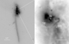 |
Fig. 1 Left: HST/ACS I (F814W) band image of Mrk 273. The image orientation is north up, east to the left. The box indicates the zoomed region in the right panel. Right: the nuclear region of Mrk 273 is shown. Positions of the three radio components, N, SW, and SE (Condon et al. 1991) are denoted by plus symbols. Much of the far-infrared emission arises from the N nucleus while Chandra imaging found the SW nucleus to be a primary hard X-ray source (see Iwasawa et al. 2011 for X-ray source identification). |
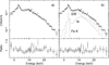 |
Fig. 2 Panel a: count rate spectrum of Mrk 273 from NuSTAR plotted with the best-fit absorbed power-law model (Model (i) of Table 1 in histogram). The model includes a Gaussian line for the Fe K line at 6.4 keV. The data to model ratio is plotted in the bottom line. The best-fit slope is very hard (Γ = 1.26). Panel b: the same data plotted with the two source model, Model (iii). The best-fit models for the two absorbed continuum sources (labelled SW and N) and the total Fe K line (labelled Fe K) are drawn in light grey histograms. |
2 NuSTAR spectrum
The NuSTAR mission observed Mrk 273 during guaranteed time on 2013 November 14 (ObsID 6000202802). We used cleaned event files processed by nupipeline using the latest calibration files. The net exposure time is 70 ks for both FPMA and FPMB modules. After checking that the spectra from the two modules agree within errors, we used the averaged spectrum for the spectral analysis below. The data above 4 keV are used to avoid any extranuclear emission in the soft band. We binned the spectrum so that each bin has more than 32 source counts and used the χ2 minimization method to search for best fits. The errors quoted in each parameter are of 1σ.
First, the 4–40 keV spectrum is fitted by a power law modified by a cold absorber in the line of sight. Various effects of Compton scattering in the absorbing medium, for example, reflected continuum emission when a torus-type geometry is assumed for an absorber, are ignored here. This is to give an idea of the spectral shape and to make a direct comparison of the result with the general properties of AGN possible, as X-ray survey data are usually analysed in this way. A narrow Gaussian is added to describe the 6.4 keV Fe K line. Figure 2a shows the NuSTAR data and the deviation from the best-fitting absorbed power-law model, which finds Γ = 1.26 ± 0.10 and NH = (3.0 ± 0.6) × 1023 cm−2 (as measured in the galaxy rest frame). The remarkably hard spectral slope is the primary characteristic that led us to seek an alternative explanation involving double AGN, as argued in Sect. 1. The Fe K line is found at rest energy of 6.39 ± 0.06 keV with intensity of (4.6 ± 1.0) × 10−6 ph cm−2 s−1. The equivalent width (EW) of the line to the absorbed continuum is 0.36 ± 0.08 keV. We note that this model systematically overestimates the data in the 7−9 keV range, where the Fe K absorption edge (the threshold energy at 7.1 keV for neutral Fe) is present. The above fit of the absorbing column is primarily driven by the continuum rollover at the low energy side. The mismatch ofthe Fe K absorption band indicates that the Fe absorption edge is deeper than predicted by the best-fit NH. This can beexplained by increased Fe metallicity (relative to the solar abundance of Anders & Grevesse 1989). While other elements are tied together and independent from Fe, when Fe K metallicity is fitted NH(Fe) is found to be (4.5 ± 0.9) × 1023 cm−2, while NH = (3.2 ± 0.5) × 1023 cm−2 for the other elements. Although statistical evidence for excess Fe metallicity is not strong, it is suggestive for the proposed two-component model as discussed below.
In Sect. 1, we mentioned the possible presence of a Compton-thick AGN in the N nucleus in addition to the SW nucleus, suggesting that the hard NuSTAR continuum as measured above may result from elevated continuum emission above 10 keV due to a strongly absorbed source in N. Here, a surmised N source would have NH ~ 1024 cm−2. The above inspection of the NuSTAR spectrum gives two more properties to favour this hypothesis: the deep Fe K absorption edge and the large EW of the Fe K line; however, these properties are not as strong as the spectral slope. An additional strongly absorbed source would enhance the total Fe edge depth without invoking the excess Fe metallicity. The observed Fe line EW of 0.36 keV is larger than expected for an absorbing torus with NH ~ 3 × 1023 cm−2 (EW ≃ 0.2 keV; Ikeda et al. 2009; Ghisellini et al. 1994; Awaki et al. 1991). In fact, the spectral fit using the MYTORUS model presented in Teng et al. (2015) appears to underestimate the Fe K line flux (their Fig. 5). Extra line emission from N, as hinted by the Chandra observation (see Sect. 1), could account for the excess line emission.
We proceed to model the NuSTAR spectrum with two absorbed nuclei, SW and N. The N nucleus is hypothesized to have an X-ray source absorbed by a larger NH than that for SW. We assume that each nucleus has an X-ray source with the standard power-law slope of Γ = 1.9 (e.g. Nandra & Pounds 1994; Ueda et al. 2014). Effects of reflection within the respective absorbers computed by Monte Carlo simulations assuming a torus geometry (e-torus: Ikeda et al. 2007; details of the usage are described in Awaki et al. 2009) are included. Fe K line emission, which is not included in e-torus, is modelled by a Gaussian, which accounts for a sum of the line emission from both nuclei. Since the inclination and opening angles of the tori of the respective nuclei cannot be constrained independently, we made the following assumptions of the torus geometry: both tori are inclined at 55° (which is the inclination angle measured for the gas disc at N by U et al. 2013 but not known for SW); the opening angles are 50° for SW and 10° for N, as a relatively large opening of the torus is expected for SW exhibiting Seyfert 2 characteristics (Colina et al. 1999; U et al. 2013) while a small opening for the dense-gas filled N nucleus. Solar metallicity is assumed for both absorbers.
This double source model describes the data well (Fig. 2b), and the quality of fit is comparable to or even better than those single source models (Table 1). The model agrees with the Fe K absorption band well. The assumed steep spectral slope fits better the data at the high energy end (25−40 keV), which results in a slightly smaller χ2 than in Model (ii). The absorbing columns are found to be NH = 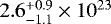 cm−2 for SW and NH =
 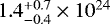 cm−2 for N. The fit suggests that the hypothetical N nucleus is absorbed by a Thomson depth of unity, in agreement with a suspected Compton-thick AGN. According to the fit, 87 per cent of the observed 4−8 keV flux comes from the SW component while the N component, which is faint at lower energies, rises sharply towards 10 keV and exceeds SW at ~ 12 keV upwards (see Fig. 2b). The observed 4−8 keV and 10−30 keV fluxes and the intrinsic continuum source luminosities in the 2−10 keV bands for the SW and N components, estimated from the fit, are given in Table 2. Intrinsically, the hidden N nucleus appears to be a factor of 2 more luminous than the SW nucleus.
The measured Fe K line flux found in the above fit is (4.1 ± 1.0) × 10−6 ph cm−2 s−1; there are contributions from both nuclei. According to Ikeda et al. (2009), EW = 0.18 keV is expected for an illuminated torus with NH = 2.6 × 1023 cm−2, as obtainedfor SW. The corresponding line intensity is 2.2 × 10⁻⁶ ph cm−2 s−1. The rest of the line flux ((1.9 ± 1.0) × 10−6 ph cm−2 s−1) can then beattributed to N. The corresponding EW with respect to the N continuum is EW ≃ 0.7 keV, which is expected for NH ≃ 1 × 1024 cm−2, in agreement with the estimated NH for N. The same spectral fit using absorption and reflection spectra with Fe line emission, computed by other codes, for example, MYTORUS (Murphy & Yaqoob 2009) instead of e-torus gives a consistent result.
The spectrum taken from the region of the N nucleus in the earlier Chandra observation shows marginal evidence of a strong 6.4 keV line (Iwasawa et al. 2011) with intensity of 1.4 ± 0.7 ph cm−2 s−1, which is comparable to the above estimate of the Fe line in N based on the NuSTAR. In addition to emission from a putative AGN, the strong starburst taking place in N could generate hot gas emitting high-ionization Fe (mainly Fe xxv) emission, which may contribute to the 6−7 keV image extension towards N seen by Chandra. There are strong cases for such high-ionization Fe emission in the ULIRG Arp 220 (Iwasawa et al. 2005, 2009; Teng et al. 2009, 2015) and the LIRG NGC 3690E (Ballo et al. 2004; Ptak et al. 2015). Assuming the high-ionization Fe emission is proportional to star formation rate, we estimated its line flux based on the measurements for Arp 220 and NGC 3690E, taking into account the source distances. This line flux is found to be (4− 8) × 10−7 ph cm−2 s−1, that is approximately 10−20% of the total line flux detected with NuSTAR.
3 Spectral variability
There are previous X-ray observations of Mrk 273 mainly at energies lower than 10 keV and the source flux is variable. According to the spectral decomposition, while the observed continuum flux below 10 keV is dominated by SW, the two nuclei may have comparable contributions to the Fe K line. Spectral variability, including the Fe line, accompanied by total X-ray brightness changes may provide a clue to the reality of two-component modelling. We used four other X-ray observations of Mrk 273 performed with the Chandra X-ray Observatory (Chandra), Suzaku, and XMM-Newton between 2000 and 2013 (Table 3, they are labelled c00, x02, s06, and x13). There are two XMM-Newton observations, one of which (x13) was carried out simultaneously with the NuSTAR observation (n13). The 4−10 keV data of the EPIC pn and two MOS cameras of XMM-Newton and Suzaku XIS and the 4−8 keV data of Chandra were used. Their spectra are shown in Fig. 3. The 4−8 keV X-ray source flux observed in c00 dropped significantly during x02 and s06 and then recovered during x13 and n13.
Among these previous observations, marginal detection in the 15−40 keV band with the Suzaku HXD-PIN during s06 (Teng et al. 2009) may have potential significance to our hypothesis. Our own analysis (with the 2009-Aug. version of hxdpinxbpi and the “tuned” ver. 2.0 background) obtained 15−40 keV flux of (4.3 ± 1.1) × 10−12 erg s−1 cm−2 (the error is statistical uncertainly only) and the spectral data are plotted in Fig. 4, along with the 3−10 keV XIS data taken in the same observation and the NuSTAR data. The source excess (~ 3%) is slightly larger than the systematic uncertainty of the background (~1.3% in 15−40 keV; Mizuno et al. 2008)and the detection remains marginal. Supposing this PIN measurement is real, Fig. 4 shows that the observed 15−40 keV flux is comparable between s06 and n13 (f15−40 = (3.3 ± 0.3) × 10−12 erg s−1 cm−2), whilst the Suzaku XIS flux below 10 keV is more than a factor of 2 fainter than that of NuSTAR (see Table 4). This uncorrelated variability above and below 10 keV suggests two distinct sources are present in the respective bands, subject to the reliability of the PIN detection, in agreement with the NuSTAR spectral decomposition (Fig. 2b). In the double source picture, the SW source is variable while the N source maintains similar brightness. The same spectral model fitted to the NuSTAR data (Model (iii) of Table 1) gives a good description of the Suzaku spectrum by changing only the continuum normalization for SW and the Fe line flux.
Now we look at spectral variability below 10 keV between the four observations via a simple modelling. All the spectra are modelled byan absorbed power law plus a narrow Gaussian for the Fe K line. We assume a power-law slope of Γ = 1.26 obtained from the NuSTAR spectrum (Sect. 2). The column density of cold absorber NH, power-law normalization and Fe line strength are left variable between the observations. If SW is solely responsible for the observed X-ray emission, the measured NH is the absorbing column towards the SW nucleus, while in the context of the double source model, it is a measure of spectral hardness in the 4−10 keV band of the summed spectrum of both nuclei. The spectral shown in Fig. 3 have been corrected for the detector response curve (Iwasawa et al. 2012) and when data from multiple detectors are available (XMM-Newton EPIC, and Suzaku XIS), they are averaged for the convenience of a visual comparison. Spectral fitting was performed for uncorrected data from the individual detectors jointly, using the detector responses and background to obtain the spectral parameters of interest. The absorbing column density, Fe line intensity, and 4−8 keV flux estimated from the spectral fits are shown in Table 4.
Among the four observations, the continuum source is bright in c00 and x13 and faint in x02 and s06. The variability results on NH and Fe line flux between the bright and faint states appear to be more consistent with the “SW + N” hypothesis than that of SW alone, as explained below.
The Fe line flux dropped when the 4−8 keV continuum flux was low (x02 and s06) and rose back when the continuum brightened (x13), suggesting that the line responds to the continuum illumination. However, the correlation plot (Fig. 5) shows a positive offset in line flux at zero continuum intensity. As the SW nucleus dominates the observed 4−8 keV continuum, the continuum variability should be driven by SW. The responding Fe line is therefore attributed to that from SW and the offset line flux (≃ 1.4 × 10⁻⁶ ph cm−2 s−1) can be considered to originate from N. This line flux decomposition roughly agrees with that from the EW argument for the NuSTAR data (Sect. 2). This interpretation relies on the condition that the Fe line emitter in SW lies sufficiently close to the central source so that it follows the continuum variability within the intervals between the observations (a few years, corresponding to a ~pc in physical scale).
Spectral fits to the NuSTAR data.
On the other hand, the inferred NH is larger when the 4−8 keV flux is low (Table 4). In the dual AGN scenario, this would be a natural consequence. When the 4−8 keV flux, which is largely due to SW, is lowered, a relative contribution of the more strongly absorbed N became larger because N appears to remain in similar flux level, as discussed above (see Fig. 4); this results in a harder spectrum that manifests itself as a larger absorbing column as measured. We assume that column densities obscuring the two nuclei remain the same, which may not necessarily hold. The variability of NH in absorbed AGN is not uncommon (e.g. Risaliti et al. 2002). However, since the absorbing clouds in the line of sight do not know what the continuum source does, NH variability should be independent of the continuum flux and any correlated behaviour with continuum brightness as seen here would not exist. A larger number of measurements are needed to test the randomness of NH variability.
In summary, the disconnected flux variability below and above 10 keV seen between s06 and n13 appears to support two distinct sources, as inferred by the NuSTAR spectral decomposition, indicating that the SW source is significantly variable while the N source is more stable between the observations. The Fe K line flux and the spectral hardness, as a function of source brightness, also behave as expected from the double source hypothesis, under reasonable conditions.
4 Discussion
If the SW nucleus alone accounts for the X-ray emission of Mrk 273 observed with NuSTAR, some extreme conditions are required to produce the unusually hard continuum slope and the excess Fe metallicity. For the former, for instance, a compact corona (thus injection of soft photons from the disc is minimized) with a large optical depth, for example, τ ~ 10, may be a requirement. Blazar-like jet emission, which could produce a hard X-ray spectrum, is unlikely because SW is a weak radio source (Condon et al. 1991). While SW as the sole X-ray source cannot be ruled out, the introduction of an additional, strongly absorbed X-ray source hypothesized in N, offers a more natural explanation for the NuSTAR spectrum with X-ray characteristics that are normal for AGN (Sect. 2) and various spectral variabilities (Sect. 3). U et al. (2013) also argued for a buried AGN in N, using the H2 outflow energetics and the photoionization condition inferred from the [Si vi]/Brγ ratio (see also Rodríguez Zaurín et al. 2014) in support of the putative Compton-thick AGN. It might be possible to test the two source hypothesis/scenario with Fe K narrowband imaging (Iwasawa et al. 2011) of improved data quality (new 200 ks Chandra data have been acquired recently; PI: S. Veilleux), but we probably have to wait for imaging with a future high-resolution hard X-ray telescope to be decisive.
The 2–10 keV absorption-corrected luminosity of the hypothetical N nucleus is estimated to be 1.3 × 1043 erg s−1, comparable to Seyfert nuclei. The bolometric AGN luminosity of N is then ~ 2 × 1044 erg s−1 when the bolometric correction of Marconi et al. (2004) is used. It is about two orders of magnitude below the total infrared luminosity, indicating that the AGN does not dominate the total energy production in Mrk 273. With a black hole mass of 1 × 10⁹ M⊙, the Eddington ratio is about 10−3. NGC 6240 is a well-known example of a double AGN system in LIRGs with two Compton-thick nuclei (Komossa et al. 2003). If proved true, the double AGN in Mrk 273 would be similar to those found in LIRGs Mrk 266 (Mazzarella et al. 2012)and IRAS 20210+1121 (Piconcelli et al. 2010), in which one of the two AGN in each system is Compton thick.
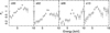 |
Fig. 3 X-rayspectra of Mrk 273 observed at the four epochs (Table 3). The data are plotted in flux density unit of 10−13 erg s−1 cm−2 keV−1. |
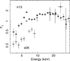 |
Fig. 4 Same as Fig. 3 but the Suzaku XIS (open circles) and PIN (open squares) data from s06 are plotted with the NuSTAR broadband data (filled squares). |
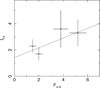 |
Fig. 5 Correlation diagram of the Fe K line and 4−8 keV continuum fluxes between the four observations. The 4−8 keV continuum flux and the Fe line intensity are in units of 10−13 erg s−1 cm−2 and 10−6 ph cm−2 s−1, respectively. |
Decomposed fluxes and luminosities.
X-ray observations of Mrk 273.
Variability between four obserations.
Acknowledgements
This research made use of data obtained from NuSTAR, Chandra X-ray Observatory, XMM-Newton and Suzaku, reduced and analysed by software provided by HEASARC, the Chandra X-ray Center, and the XMM-Newton Science Operation Centre. K.I. acknowledges support by the Spanish MINECO under grant AYA2016-76012-C3-1-P and MDM-2014-0369 of ICCUB (Unidad de Excelencia “María de Maeztu”). V.U. acknowledges funding support from the University of California Chancellor’s Postdoctoral Fellowship. Support for AMM is provided by NASA through Hubble Fellowship grant #HST-HF2-51377 awarded by the Space Telescope Science Institute, which is operated by the Association of Universities for Research in Astronomy, Inc., for NASA, under contract NAS5-26555.
References
- Anders, E., & Grevesse, N. 1989, Geochim. Cosmochim. Acta, 53, 197 [Google Scholar]
- Awaki, H., Koyama, K., Inoue, H., & Halpern, J. P. 1991, PASJ, 43, 195 [NASA ADS] [Google Scholar]
- Awaki, H., Terashima, Y., Higaki, Y., & Fukazawa, Y. 2009, PASJ, 61, S317 [NASA ADS] [CrossRef] [Google Scholar]
- Balestra, I., Boller, T., Gallo, L., Lutz, D., & Hess, S. 2005, A&A, 442, 469 [NASA ADS] [CrossRef] [EDP Sciences] [Google Scholar]
- Ballo, L., Braito, V., Della Ceca, R., et al. 2004, ApJ, 600, 634 [NASA ADS] [CrossRef] [Google Scholar]
- Barnes, J. E., & Hernquist, L. 1992, ARA&A, 30, 705 [NASA ADS] [CrossRef] [Google Scholar]
- Bondi, M., Pérez-Torres, M.-A., Dallacasa, D., & Muxlow, T. W. B. 2005, MNRAS, 361, 748 endrefcommentnewpage [NASA ADS] [CrossRef] [Google Scholar]
- Carilli, C. L., & Taylor, G. B. 2000, ApJ, 532, L95 [NASA ADS] [CrossRef] [PubMed] [Google Scholar]
- Colina, L., Arribas, S., & Borne, K. D. 1999, ApJ, 527, L13 [NASA ADS] [CrossRef] [PubMed] [Google Scholar]
- Condon, J. J., Huang, Z.-P., Yin, Q. F., & Thuan, T. X. 1991, ApJ, 378, 65 [NASA ADS] [CrossRef] [Google Scholar]
- Downes, D., & Solomon, P. M. 1998, ApJ, 507, 615 [NASA ADS] [CrossRef] [Google Scholar]
- Ghisellini, G., Haardt, F., & Matt, G. 1994, MNRAS, 267, 743 [NASA ADS] [CrossRef] [Google Scholar]
- Haardt, F., & Maraschi, L. 1993, ApJ, 413, 507 [NASA ADS] [CrossRef] [MathSciNet] [Google Scholar]
- Hopkins, P. F., Hernquist, L., Cox, T. J., et al. 2005, ApJ, 630, 705 [NASA ADS] [CrossRef] [Google Scholar]
- Ikeda, S., Awaki, H., & Terashima, Y. 2009, ApJ, 692, 608 [NASA ADS] [CrossRef] [Google Scholar]
- Iwasawa, K. 1999, MNRAS, 302, 96 [NASA ADS] [CrossRef] [Google Scholar]
- Iwasawa, K., Sanders, D. B., Evans, A. S., et al. 2005, MNRAS, 357, 565 [NASA ADS] [CrossRef] [Google Scholar]
- Iwasawa, K., Sanders, D. B., Evans, A. S., et al. 2009, ApJ, 695, L103 [NASA ADS] [CrossRef] [Google Scholar]
- Iwasawa, K., Mazzarella, J. M., Surace, J. A., et al. 2011, A&A, 528, A137 [NASA ADS] [CrossRef] [EDP Sciences] [Google Scholar]
- Iwasawa, K., Mainieri, V., Brusa, M., et al. 2012, A&A, 537, A86 [NASA ADS] [CrossRef] [EDP Sciences] [Google Scholar]
- Klöckner, H.-R., & Baan, W. A. 2004, A&A, 419, 887 [NASA ADS] [CrossRef] [EDP Sciences] [Google Scholar]
- Komossa, S., Burwitz, V., Hasinger, G., et al. 2003, ApJ, 582, L15 [NASA ADS] [CrossRef] [Google Scholar]
- Marconi, A., Risaliti, G., Gilli, R., et al. 2004, MNRAS, 351, 169 [NASA ADS] [CrossRef] [Google Scholar]
- Mazzarella, J. M., Iwasawa, K., Vavilkin, T., et al. 2012, AJ, 144, 125 [NASA ADS] [CrossRef] [Google Scholar]
- Mizuno, T., Fukazawa, Y., Takahashi, H., et al. 2008, JX ISAS Suzaku Memo [Google Scholar]
- Murphy, K. D., & Yaqoob, T. 2009, MNRAS, 397, 1549 [NASA ADS] [CrossRef] [Google Scholar]
- Nandra, K., & Pounds, K. A. 1994, MNRAS, 268, 405 [NASA ADS] [CrossRef] [Google Scholar]
- Piconcelli, E., Vignali, C., Bianchi, S., et al. 2010, ApJ, 722, L147 [NASA ADS] [CrossRef] [Google Scholar]
- Ptak, A., Heckman, T., Levenson, N. A., Weaver, K., & Strickland, D. 2003, ApJ, 592, 782 [NASA ADS] [CrossRef] [Google Scholar]
- Ptak, A., Hornschemeier, A., Zezas, A., et al. 2015, ApJ, 800, 104 [NASA ADS] [CrossRef] [Google Scholar]
- Risaliti, G., Elvis, M., & Nicastro, F. 2002, ApJ, 571, 234 [NASA ADS] [CrossRef] [Google Scholar]
- Rodríguez Zaurín, J., Tadhunter, C. N., Rupke, D. S. N., et al. 2014, A&A, 571, A57 [NASA ADS] [CrossRef] [EDP Sciences] [Google Scholar]
- Sanders, D. B., & Mirabel, I. F. 1996, ARA&A, 34, 749 [NASA ADS] [CrossRef] [Google Scholar]
- Scoville, N. Z., Evans, A. S., Thompson, R., et al. 2000, AJ, 119, 991 [NASA ADS] [CrossRef] [Google Scholar]
- Teng, S. H., Veilleux, S., Anabuki, N., et al. 2009, ApJ, 691, 261 [NASA ADS] [CrossRef] [Google Scholar]
- Teng, S. H., Rigby, J. R., Stern, D., et al. 2015, ApJ, 814, 56 [NASA ADS] [CrossRef] [Google Scholar]
- U, V., Medling, A., Sanders, D., et al. 2013, ApJ, 775, 115 [NASA ADS] [CrossRef] [Google Scholar]
- Ueda, Y., Akiyama, M., Hasinger, G., Miyaji, T., & Watson, M. G. 2014, ApJ, 786, 104 [NASA ADS] [CrossRef] [Google Scholar]
- Xia, X. Y., Xue, S. J., Mao, S., et al. 2002, ApJ, 564, 196 [NASA ADS] [CrossRef] [Google Scholar]
All Tables
All Figures
|
Fig. 1 Left: HST/ACS I (F814W) band image of Mrk 273. The image orientation is north up, east to the left. The box indicates the zoomed region in the right panel. Right: the nuclear region of Mrk 273 is shown. Positions of the three radio components, N, SW, and SE (Condon et al. 1991) are denoted by plus symbols. Much of the far-infrared emission arises from the N nucleus while Chandra imaging found the SW nucleus to be a primary hard X-ray source (see Iwasawa et al. 2011 for X-ray source identification). |
| In the text | |
|
Fig. 2 Panel a: count rate spectrum of Mrk 273 from NuSTAR plotted with the best-fit absorbed power-law model (Model (i) of Table 1 in histogram). The model includes a Gaussian line for the Fe K line at 6.4 keV. The data to model ratio is plotted in the bottom line. The best-fit slope is very hard (Γ = 1.26). Panel b: the same data plotted with the two source model, Model (iii). The best-fit models for the two absorbed continuum sources (labelled SW and N) and the total Fe K line (labelled Fe K) are drawn in light grey histograms. |
| In the text | |
|
Fig. 3 X-rayspectra of Mrk 273 observed at the four epochs (Table 3). The data are plotted in flux density unit of 10−13 erg s−1 cm−2 keV−1. |
| In the text | |
|
Fig. 4 Same as Fig. 3 but the Suzaku XIS (open circles) and PIN (open squares) data from s06 are plotted with the NuSTAR broadband data (filled squares). |
| In the text | |
|
Fig. 5 Correlation diagram of the Fe K line and 4−8 keV continuum fluxes between the four observations. The 4−8 keV continuum flux and the Fe line intensity are in units of 10−13 erg s−1 cm−2 and 10−6 ph cm−2 s−1, respectively. |
| In the text | |
Current usage metrics show cumulative count of Article Views (full-text article views including HTML views, PDF and ePub downloads, according to the available data) and Abstracts Views on Vision4Press platform.
Data correspond to usage on the plateform after 2015. The current usage metrics is available 48-96 hours after online publication and is updated daily on week days.
Initial download of the metrics may take a while.