| Issue |
A&A
Volume 611, March 2018
|
|
|---|---|---|
| Article Number | A81 | |
| Number of page(s) | 13 | |
| Section | Cosmology (including clusters of galaxies) | |
| DOI | https://doi.org/10.1051/0004-6361/201731447 | |
| Published online | 04 April 2018 | |
Bose–Einstein condensate haloes embedded in dark energy
1
Departamento de Física Teórica, Universidad de Zaragoza,
50009
Zaragoza,
Spain
e-mail: This email address is being protected from spambots. You need JavaScript enabled to view it.
2
BIFI, Instituto de Biofísica y Física de Sistemas Complejos, Universidad de Zaragoza,
50009
Zaragoza,
Spain
e-mail: This email address is being protected from spambots. You need JavaScript enabled to view it.
Received:
26
June
2017
Accepted:
8
December
2017
Abstract
Context. We have studied clusters of self-gravitating collisionless Newtonian bosons in their ground state and in the presence of the cosmological constant to model dark haloes of dwarf spheroidal (dSph) galaxies.
Aims. We aim to analyse the influence of the cosmological constant on the structure of these systems. Observational data of Milky Way dSph galaxies allow us to estimate the boson mass.
Methods. We obtained the energy of the ground state of the cluster in the Hartree approximation by solving a variational problem in the particle density. We have also developed and applied the virial theorem. Dark halo models were tested in a sample of 19 galaxies. Galaxy radii, 3D deprojected half-light radii, mass enclosed within them, and luminosity-weighted averages of the square of line-of-sight velocity dispersions are used to estimate the particle mass.
Results. Cosmological constant repulsive effects are embedded in one parameter ξ. They are appreciable for ξ > 10−5. Bound structures appear for ξ ≤ ξc = 1.65 × 10⁻⁴, what imposes a lower bound for cluster masses as a function of the particle mass. In principle, these systems present tunnelling through a potential barrier; however, after estimating their mean lifes, we realize that their existence is not affected by the age of the Universe. When Milky Way dSph galaxies are used to test the model, we obtain 3.5−1.0+1.3 × 10⁻²² eV for the particle mass and a lower limit of 5.1−2.8+2.2 × 10⁶ M⊙ for bound haloes.
Conclusions. Our estimation for the boson mass is in agreement with other recent results which use different methods. From our particle mass estimation, the treated dSph galaxies would present dark halo masses ~5–11 ×107 M⊙. With these values, they would not be affected by the cosmological constant (ξ < 10−8). However, dark halo masses smaller than 107 M⊙ (ξ > 10−5) would already feel their effects. Our model that includes dark energy allows us to deal with these dark haloes. Assuming quantities averaged in the sample of galaxies, 10−5 < ξ ≤ ξc dark haloes would contain stars up to ~8–15 kpc with luminosities ~9–4 ×10³ L⊙. Then, their observation would be complicated. The comparison of our lower bound for dark halo masses with other bounds based on different arguments, leads us to think that the cosmological constant is actually the responsible of limiting the halo mass.
Key words: dark matter / dark energy / galaxies: dwarf
© ESO 2018
1 Introduction
The quantum systems of interacting bosons are interesting in relation to the fundamental question of stability of matter (Lieb & Seiringer 2009), in astrophysics as potential candidates of dark matter (Jetzer 1992), and also because they can simulate condensates of the Bose–Einstein type (Griffin et al. 1996). Ruffini & Bonazzola (1969) studied the properties of a self-gravitating Newtonian sphere of bosons by means of variational method and established an upper bound for the ground state energy of this system, namely: E0 ≤−0.1626M3G2m2ℏ−2. Here, M is the mass of the sphere, G is the gravitational constant, m, the boson mass, and ℏ, the Planck’s constant. This result was in conflict with the lower bound for the same system established by Lévy-Leblond (1969): E0 ≥−0.125M3G2m2ℏ−2. This conflict worsened when Basdevant et al. (1990) significantly improved the lower bound; they obtained E0 ≥−0.0625M3G2m2ℏ−2. In 1989, we studied the same system in the Hartree approximation, and obtained an upper bound E0 ≤−0.05426M3G2m2ℏ−2 (Membrado et al. 1989), which brought peace with the mentioned lower bounds: the correction of a factor three had the answer.
Recently, Hui et al. (2017) have solved the time-independent Schrödinger–Poisson equation for its lowest eigenstates, assuming spherical symmetry. The energy per particle of the ground eigenstate that they obtained is the same we derived in Membrado et al. (1989). Our upper bound coincides with the total energy of the ground state they obtained when the phase of the wave function is position independent.
Using a simple method, Membrado & Pacheco (2012) estimated a limit for the existence of those Newtonian boson clusters in the presence of dark energy. We imposed that the critical distance where the attractive gravitational effect is balanced by the repulsion exerted by the cosmological constant must be greater than the cluster length scale.
Scalar fields fulfilling different potentials and masses ranging from 10−26 eV up to 10−23 eV have been proposed to model dark matter (see, for example: Lee & Koh 1996; Sahni & Wang 2000; Matos & Ureña-López 2000; Matos & Arturo Ureña-López 2001). We should also mention the work by Amendola & Barbieri (2006), who proposed that part of dark matter may be an ultra-light pseudo-Goldstone-boson with a mass m ≥ 10−23 eV, arising fromthe spontaneous breaking at a scale close to the Planck’s mass of an extended approximate symmetry.
It so happens that the standard cosmological constant and cold dark matter model (ΛCDM), at scale of individual galaxies smaller than 10 kpc, produces an excess of dwarf galaxies and singular galactic cores not supported by observations(see, e.g. Weinberg et al. 2015). Hu et al. (2000) showed that these problems could be solved by introducing fuzzy dark matter (FDM) instead CDM. This FDM would be constituted by ultra-light scalar particles with a mass in the order of 10−22 eV, initially in a Bose–Einstein condensate. For a thorough list of references on this subject, see Chavanis (2011). The physics that support this new model and its astrophysical consequences are reviewed and analysed by Hui et al. (2017).
In Membrado & Pacheco (2013), we applied a dark halo made of collisionless Newtonian bosons to the ultra-faint Milky Way satellite galaxy Segue 1 (Simon et al. 2011; Martinez et al. 2011). We saw that when taking its half-light radius, r1∕2, as the radius that covers 99% of the dark assembly mass, the Segue 1 mass at r1∕2 can be reproduced. Thus, we derived an upper bound for the boson mass, m < 10−20 eV.
Chen et al. (2017) applied Jeans analysis to the kinematic data of eight classical dwarf spheroidal (dSph) galaxies, assuming a soliton core profile (Schive et al. 2014) connecting to a Navarro–Frenk–White profile (Navarro et al. 1997) at larger radii. They obtain masses between  eV (for Draco) and
  eV (for Sextans).
Calabrese & Spergel (2016) applied the same model than Chen et al. (2017) to Draco II and Triangulum II, but using two observational limits: the half-light mass, M1∕2 (Wolf et al. 2010), and the maximum halo mass, Mmax ~ 2 × 10¹⁰ M⊙, based on the mass function of the Milky Way dwarf satellite galaxies (Giocoli et al. 2008). They find that if the stellar component is within the core, the particle mass would be about m ~ 3.7–5.6 ×10⁻²² eV.
In this paper, we have retaken and extended the calculation made in Membrado & Pacheco (2013) to 19 dSph galaxies. We have dealt with a sphere of self-gravitating bosons as in Membrado et al. (1989), but have assumed the presence of dark energy. The aim of this paper is: (1) to determine the effects of the cosmological constant; and (2) to estimate the boson mass.
The paper is organized as follows. In Sect. 2, we present a Hartree-like method which allows us to obtain the energy per unit mass of the ground state of a self-gravitating assembly of identical bosons in the presence of the cosmological constant. In this section, the Hartree method is stated as a variational problem in the particle density. The solutions for the particle number density are shown in Sect. 3. The virial theorem for these systems is treated in Sect. 4. In Sect. 5, we use clusters of self-gravitating collisionless Newtonian bosons to model dark haloes of dSph galaxies. Finally, our main conclusions are summarized in Sect. 6.
2 The single-boson energy equation in boson clusters embedded in dark energy
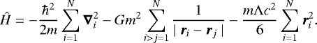
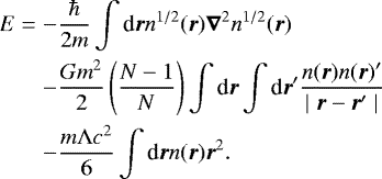
Let us consider an assembly of N self-gravitating identical bosons with mass m and dark energy. Assuming Newtonian gravity for matter and the cosmological constant model for dark energy, the Hamiltonian of the system is
 (1)
(1)
In Eq. (1), Λ is the cosmological constant; for the cosmological constant term, see, for example, Membrado & Pacheco (2012).
For the ground state of the system, ∣ψ⟩, its energy, E, is
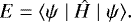 (2)
(2)
In the Hartree approximation, the particle density, n(r), at the point r is given by
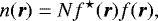 (3)
(3)
where ![Mathematical equation: $f = [n / N ]^{1/2}$](/articles/aa/full_html/2018/03/aa31447-17/aa31447-17-eq8.png) is the single-particle wave function (we note that f is real because corresponds to a bound state). Thus
is the single-particle wave function (we note that f is real because corresponds to a bound state). Thus
 (4)
(4)
Henceforth, we assume that N ≫ 1.
The minimum energy solution can be expressed as a variational problem. Thus, E, given by Eq. (4), must be minimized as a function of n(r) with the constraint
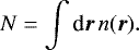 (5)
(5)
Hence, we deal with
![Mathematical equation: \begin{equation*}\delta ( E[n] + \lambda N[n]) = 0, \end{equation*}](/articles/aa/full_html/2018/03/aa31447-17/aa31447-17-eq11.png) (6)
(6)
where λ is the Lagrange multiplier. Assuming spherical symmetry and radius R, the variational problem given by Eq. (6) is of the kind
![Mathematical equation: \begin{equation*}\delta \int_0^R F[n] \textrm{d}r = 0, \end{equation*}](/articles/aa/full_html/2018/03/aa31447-17/aa31447-17-eq12.png) (7)
(7)
where  , a dot meaning differentiation with respect to r. Explicitly,
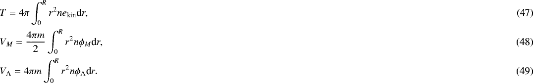
![Mathematical equation: \begin{equation*}F = 4\pi r^2 n \left[e_{\textrm{kin}} + {1\over 2} m \phi_{M} + m \phi_{{\UpLambda}} + \lambda\right]. \end{equation*}](/articles/aa/full_html/2018/03/aa31447-17/aa31447-17-eq14.png) (8)
(8)
In Eq. (8), ekin, ϕM, and ϕΛ are the kinetic energy per particle, the gravitational potential due to matter, and the gravitational potential due to dark energy, respectively. They are given by
![Mathematical equation: \begin{eqnarray}&&e_{\textrm{kin}} = -{\hbar^2\over 2m}\left[{\dot n\over nr} -{\dot n^2\over 4 n^2} + {\ddot n\over 2n}\right], \\ &&\phi_M = - G m \left[ {1\over r}\int_0^r n r'^2 \textrm{d}r' + \int_r^R n r' \textrm{d}r'\right], \\ &&\phi_{{\UpLambda}} = - {1\over 6} \UpLambda c^2 r^2. \end{eqnarray}](/articles/aa/full_html/2018/03/aa31447-17/aa31447-17-eq15.png)
The solution of the variational problem is shown in Appendix A. Thus, using Eq. (8) in (A.9), the boson number density, n(r), must fulfil
 (12)
(12)
It should be noticed that e in Eq. (12) is the energy of the single-particle wave function f; that is,
![Mathematical equation: \begin{equation*}\left[ -{\hbar^2\over 2 m}\vec{\nabla}^2 + m \phi_M + m \phi_{{\UpLambda}}\right] f = e f. \end{equation*}](/articles/aa/full_html/2018/03/aa31447-17/aa31447-17-eq17.png) (13)
(13)
We take
 (14)
(14)
as the length scale of a cluster of mass M that contains N identical bosons of mass m (i.e. M = Nm). This quantity allows us to define dimensionless variables η and x as

As the mass enclosed within a sphere of radius r is
 (17)
(17)
using Eqs. (15) and (16) we define the dimensionless mass
 (18)
(18)
fulfilling
 (19)
(19)
Hence, Eq. (5) reads as
 (20)
(20)
We also introduce the dimensionless parameters ϵ and ξ given by

In Eq. (21), ϵ is the dimensionless energy of the single-particle wave function. The parameter ξ, defined in Eq. (22), is a measure of the influence of the cosmological constant repulsive effect with respect to the attractive effect due to matter. From Eqs. (14) and (22), the mass of the cluster can be expressed as a function of m and ξ by
 (23)
(23)
Using Eqs. (14)–(16) and (21)–(22), Eq. (12) reads as
![Mathematical equation: \begin{eqnarray}&&\epsilon = \kappa(x) + \nu_M(x) + \nu_{{\UpLambda}}(x), \\ &&\kappa(x) = - \left[ {\eta' \over \eta x} - {\eta'^2\over 4 \eta^2} + {\eta''\over 2 \eta } \right ], \\ &&\nu_M(x) = -{\mu(x)\over x} - \int_{x}^{(R/b)} n(y) y \textrm{d}y, \\ &&\nu_{{\UpLambda}}(x) = - {\xi\over 6} x^2, \end{eqnarray}](/articles/aa/full_html/2018/03/aa31447-17/aa31447-17-eq26.png)
In Eq. (24), κ(x) is dimensionless kinetic energy per particle (an apostrophe means differentation with respect to x); νM (x) and νΛ (x) are dimensionless gravitational energies per particle due to matter and dark energy, respectively.
When the cosmological constant contribution is neglected, the solution of Eq. (24) must not have any node (1s state), so η(x →∞) → 0 (see Fig. 1 of Membrado et al. 1989). Such a solution has a classical turning point at x = x1, where k(x1) = 0 (see Fig. 1). From the single-particle wave function, f, the probability of finding the particle inside the volume of dimensionless radius x is given by μ(x) (see Eq. (18)). As μ(x1) = 0.83, the probability of finding it beyond the classical turning point cannot be considered as negligible.
When ξ≠0, the cosmological constant term of the gravitational energy makes the kinetic term be also zero at some x = x2, beyond the classical turning point (see right hand panels of Fig. 3). This means that there could be a tunnelling process through the potential barrier from x = x1 up to x = x2. The values of the wave function, f, at x = x1 and x = x2 will allow to estimate the mean life of the system.
In the absence of dark energy, the mass density decays as x−4; that is, it vanishes at an infinite distance from the origin. Considering the virial theorem of this system at x = ∞, the result is the canonical form 2T = −V, where T is kinetic energy, and V, gravitational energy (see Membrado et al. 1989). In the case of not using the endpoint at infinity, the canonical virial relation should have to be corrected by a surface term.
When the cosmological constant is taken into account, we see in Sect. 4 that 2T = −V + 2VΛ (the final term corresponds to the cosmological constant contribution) is fulfilled at x2. This means that surface terms are null there and indicates that x2 is the dimensionless radius of the system.
From Eqs. (24)–(27) together with Eq. (20), the dimensionless distance x2 and the classical turning point, x1, fulfil

Finally, the distance x0, where the attractive gravitational effect is balanced by the repulsion (i.e. where  ), fulfils
 (30)
(30)
If we assume that for x0 ≤ x ≤ x2, the contribution of η(x) to the particle number is very small (i.e. μ(x0) ≈ 1), and that x0 ≫ 1,
 (31)
(31)
in other words
 (32)
(32)
This distance r0 is the same as that derived assuming a point mass M (see, for example: Membrado & Pacheco 2012). In Membrado & Pacheco (2012), we concluded that for r > r0, the stability of any self-gravitational cluster of matter would be affected by the cosmological constant. In this work, we see that at x0, the potential energy per particle, vM + vΛ, shows a maximum. This should cause the system to lose particles by tunnelling. Hence, the instability would be manifested in this quantum system by the loss of bosons. The ratio between the mean life of the system and the Hubble time will inform us of the importance of this instability (see Sect. 3).
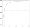 |
Fig. 1 For ξ = 0, gravitational energy, νM and single-particle energy, ϵ, as a functionof the dimensionless distance x. The classicalturning point x1 is marked. |
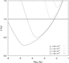 |
Fig. 2 Choice of a0 for different values of ξ (see text). |
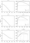 |
Fig. 3 Left panels: dimensionless particle number density, η, as a functionof x, for three values of ξ. The bottom panel corresponds to the critical value ξc. Right panels: dimensionless energies per particle for the same values of ξ shown in left panels (gravitational energy due to matter, νM; total gravitational energy, νM + νΛ; single-particle energy, ϵ), as a functionof the dimensionless distance x. The distances x1, x0 and x2 for ξc are marked in the bottom right panel. |
3 Solutions for the particle number density
Equation (24) is an integro-differential equation. Instead of solving it, we apply the dimensionless Laplacian operator, b2 ∇2, to Eq. (24) to obtain the following four-order differential equation
![Mathematical equation: \begin{eqnarray*} \eta '''' &=& 2\eta^2 \left[1 - {\xi\over \eta}\right] - {4 \eta ''' \over x} + {10 \eta ' \eta '' \over x \eta} - {6 \eta '^3 \over x \eta } + {3 \eta ' \eta '''\over n} \nonumber \\ && + {2 \eta ''^2\over\eta} - {7 \eta'^2 \eta''\over \eta^2} + {3\eta'^4\over \eta^3}.\end{eqnarray*}](/articles/aa/full_html/2018/03/aa31447-17/aa31447-17-eq32.png) (33)
(33)
It can be seen that η(x → 0) = ∑ anxn; therefore, the solution of Eq. (33) requires knowledge of a0, a1, a2, and a3. From Eqs. (24) and (33), we obtain a1 = 0 and ![Mathematical equation: $a_3 = (a_1/a_0)[(5/6)a_2 - (1/4)(a_1^2/a_0)]$](/articles/aa/full_html/2018/03/aa31447-17/aa31447-17-eq33.png) , respectively; hence a3 = 0, too. Thus, the problem is reduced to finding a0 and a2. For this subject, we chose a value for a0 and seek its corresponding a2 leading to a decreasing η(x) without any node up to x2. Finally, a0 is determined by imposing that N particles are contained up to x = x2.
, respectively; hence a3 = 0, too. Thus, the problem is reduced to finding a0 and a2. For this subject, we chose a value for a0 and seek its corresponding a2 leading to a decreasing η(x) without any node up to x2. Finally, a0 is determined by imposing that N particles are contained up to x = x2.
In Fig. 2, we show, for several values of ξ, the quantity μ(x2) (see Eq. (18)) as a function of a0 (the reader should remember that a2 is adequately fixed for each a0). In the figure, the line μ(x2) = 1 is also represented. Hence, the chosen value for a0 will be that fulfilling μ(x2) = 1. As can be seen from Fig. 2, for each ξ < ξc = 1.65 × 10⁻⁴, there are two values of a0 leading to μ(x2) = 1; the greatest a0, corresponding to the smallest ϵ, is chosen. As an example, let us consider the case ξ = 10−5. For this ξ, a0 = 6.811 × 10⁻³ and a0 = 3.827 × 10⁻⁵ fulfil μ(x2) = 1 for a2 = −1.7186 × 10⁻⁴ and a2 = −4.9123 × 10⁻⁸, respectively; these values lead to the dimensionless energies of the single-particle wave function, ϵ = −8.124 × 10⁻² and ϵ = −2.255 × 10⁻². As we are looking for minimum energy solution which was expressed as a variational problem in this work, the greatest value of a0 would lead to the ground state solution (the variational problem is just designed to determine the ground state, but not to excited states). In the case ξc = 1.65 × 10⁻⁴, only one a0 is allowed. For ξ > ξc, μ(x2) > 1 for any a0. This means that the cosmological constant imposes a limit for the existence of self-gravitating boson clusters. Thus, when the scale of the gravitational repulsive force due to the cosmological constant (Λc2bm), is greater than 1.65× 10⁻⁴ times the scale of the gravitational attraction force (GMm∕b2), self-gravitating boson assemblies can not be created. The condition ξ ≤ ξc imposes a constraint for the minimum mass of the cluster. Thus, from Eq. (23),
 (34)
(34)
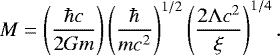
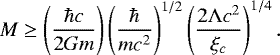
In this work, we have assumed that bosons are in Newtonian gravity. This means that (2GM∕b) ≪ c2. Hence, using Eq. (14), the mass of the cluster must fulfil
 (35)
(35)
This means that
 (36)
(36)
In Eq. (36), we have used Λ = 1.29 × 10−56 cm−2. This value is calculated from the energy density of dark energy, ρΛ, by Λ = (8πGρΛ∕c4). We have taken into account that ρΛ = ρ0ΩΛ, where 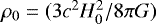 is the background energy density, H0 being the Hubble constant. Values for ΩΛ and H0 can be taken from Spergel et al. (2003); in this work we assumed ΩΛ = 0.73 and H0 = 71 km s−1 Mpc−1.
Profiles of η(x) for three values of ξ are presented in the left panels of Fig. 3. Values of a0 and a2 for the models are presented in Table 1. We have only shown density profiles for η(x) ≥ 10−8. For ξc, η(x2) = 4.7 × 10⁻⁷; and, for ξ = 10−5 and ξ = 10−6, dimensionless densities smaller than 10−8 do not already contribute to the bound particle number. The behaviour of η(x) in the neigbourhood of x2 can be seen in the bottom left panel (ξ = ξc). This behaviour is of the kind
![Mathematical equation: \begin{eqnarray}&&\eta(x\rightarrow x_2) \approx \eta(x_2)\left[1 +\alpha (x_2-x)^3\right], \\ &&\alpha = {\xi \over 9}x_2 - {1\over 3 x_2^2} > 0. \end{eqnarray}](/articles/aa/full_html/2018/03/aa31447-17/aa31447-17-eq38.png)
In the panel devoted to ξc, the profile of η(x) is finished at x = x2, where the potential barrier ends (the kinetic energy per particle is zero).
Once the particle density is known, νM(x) can be calculated from Eq. (26), and ϵ, from Eqs. (24)–(27). Then, x1 and x0 are obtained from Eqs. (29) and (30). In Table 2, x1, x0 and x2 are shown for different values of ξ. From this table, it can be seen that the greatest difference between x0 and that calculated from Eq. (31), appears for ξc, being smaller than 0.8%. This means that beyond x0, the contribution of the particle density to the number of bound particles can be considered as negligible.
In the right hand panels of Fig. 3, we present νM (x), νM (x) + νΛ(x), and ϵ for the same values of ξ treated in the left hand panels. Their profiles end at x = x2. In the figures, x1 and x0 can be observed, together with the potential barrier and the effect of the cosmological constant in the dimensionless gravitational energy per particle.
From the potential barrier, we were able to estimate the mean life of these systems, τc. This can be calculated from a timescale for the cluster, tc, and the transmission factor, T (see, for example, Matthews 1963, p. 96f). If τc is smaller than the age of the Universe, tu = 1.37 × 10¹⁰ years, these clusters should not exist at present. A timescale, tc, for the cluster is
 (39)
(39)
In Eq. (39), we have assumed non-relativistic bosons, and we have used the classical turning radius. Thus, using the transmission factor T = η(x2)∕η(x1), the mean life reads as
 (40)
(40)
Hence, using Eq. (14) in (40), bound boson clusters can exist if
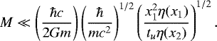 (41)
(41)
When Eq. (23) is taken into account in Eq. (41), the condition
 (42)
(42)
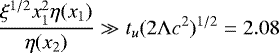
is derived. The minimum value of the left hand term of Eq. (42) happens for ξc (it is a decreasing function of ξ). For ξ = ξc = 1.65 × 10⁻⁴, x1 = 13.9, η(x1) = 2.38 × 10⁻⁴ and η(x2) = 4.69 × 10⁻⁷; thus,
![Mathematical equation: \begin{equation*}\left. { \xi^{1/2} x_1^2 \eta(x_1) \over \eta(x_2) }\right] _{\xi=\xi_c} = 1.26\times 10^3. \end{equation*}](/articles/aa/full_html/2018/03/aa31447-17/aa31447-17-eq43.png) (43)
(43)
Hence, the present existence of Newtonian boson clusters embedded in dark energy is not threatened by the age of the Universe.
Values of a0 and a2 for a different ξ.
Dimensionless distances x1, x0 and x2 for a different ξ.
4 The virial theorem
Taking the differential of Eq. (12) with respect to the radial co-ordinate, and after multiplying this result by the particle density,
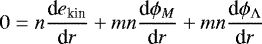 (44)
(44)
is obtained. Equation (44) is the equation of radial motion which shows the balance of strength per unit volume.
If spherical symmetry is assumed, the virial theorem is derived by first multiplying the radial motion equation by the radial co-ordinate and then integrating it over a volume. Thus, if the volume is that of a sphere of radius R, the virial theorem reads as
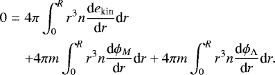 (45)
(45)
By taking R = bx2 as the radius of the system, the first term of Eq. (45) is equal to minus two times the kinetic energy of the system, T (see Appendix B; we note that, from Eq. (37), 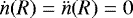 ); the second term is minus the gravitational energy due to matter, VM, calculated from the trace of the energy potential tensor of Chandrasekar (see, for example, Binney & Tremaine 1987, p. 67); the third term is two times the gravitational energy due to dark energy, VΛ (from using Eq. (11)). Thus,
 (46)
(46)
where
Equation (46) can be expressed as a function of dimensionless magnitudes,  , ṼM and ṼΛ given by
![Mathematical equation: \begin{eqnarray}&&\tilde{T} = - \int_0^{x_2} x^2 \left[{\eta'\over x} -{\eta'^2\over 4 \eta} + {\eta''\over 2}\right] \textrm{d}x, \\ &&\tilde {V}_M = -\int_0^{x_2} \eta \mu x \textrm{d}x, \\ &&\tilde {V}_{{\UpLambda}} = -{\xi \over 6} \int_0^{x_2} \eta x^4 \textrm{d}x .\end{eqnarray}](/articles/aa/full_html/2018/03/aa31447-17/aa31447-17-eq50.png)
They are related with T, VM and VΛ by
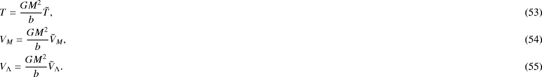
Equation (50) is obtained from Eq. (47) using Eqs. (9), (14)–(16) and (53). Equation (51) is obtained from the second term on the right hand side of Eq. (45); there, Eqs. (10), (14)–(16), (19), and (54) are used. Finally, Eq. (52) derives from Eq. (49), taking into account Eqs. (11), (14)–(16), (22), and (55). Thus,
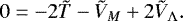 (56)
(56)
Values of  , ṼM and ṼΛ for three ξ-models are presented in Table 3.
Dimensionless total energies 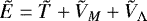 (57)
(57)
are also shown in Table 3. The total energy E, is then given by (see Eqs. (53)–(55))
 (58)
(58)
The energy, e, of the singleparticle wave function can be also obtained by multiplying Eq. (12) by the number density, n(r), and integrating it over the volume of the system. Thus,
 (59)
(59)
Then, using Eqs. (21) and (53)–(55), the dimensionless energy, ϵ, of the single particle wave function is
 (60)
(60)
Values of ϵ are also presented in Table 3. Finally, from Eqs. (56), (57) and (60), it can be seen that
 (61)
(61)
Dimensionless quantities appearing in the virial theorem and in the energy of a boson cluster.
5 Application to dark halos of dSph galaxies
Dwarf spheroidal galaxies are among the smallest and faintest galactic systems. However, their velocity dispersions suggest large mass-to-light ratios, being some of the most dark matter dominated objects in the Universe (e.g. Gilmore et al. 2007). Dwarf spheroidal galaxies have been found inside the virial radius of groups and clusters. These galaxies appear in halos of massive galaxies where tidal effects are present, so their star formation history is strongly dependent on their environment. It is generally considered that these gas-poor galaxies with old stellar population come from irregular dwarfs which have suffered processes of gas stripping and strangulation that limit further star formation.
Observational data from dSph galaxies reveal discrepancies with respect to predictions of ΛCDM models. High-resolution simulations in the standard ΛCDM cosmology (see, for example: Klypin et al. 1999; Moore et al. 1999; Diemand et al. 2007; Springel et al. 2008) predict a number ofsub-halos within the Local Group which is about two orders of magnitude higher than the total number of observed satellite galaxies (Kauffmann et al. 1993; Moore et al. 1999; Klypin et al. 1999). This result is known as the “missing satellites problem”. Simulations also lead to power-law density profiles for sub-halos (e.g. Moore et al. 1999; Navarro et al. 1997, 2004), against the more flattened profiles derived from observations (e.g. Burkert 1995; de Blok & Bosma 2002; Gentile et al. 2005; de Blok 2005). It has even been shown that tidal interactions are not able to give rise to the dSph galaxies of the Milky Way group from the most massive sub-halos in a ΛCDM Universe (Kazantzidis et al. 2004).
Moreover, dSph galaxies have also been found in isolated environments, far away from any massive galaxy (Makarov et al. 2012; Karachentsev et al. 2015). The evolution of these galaxies seems to be regulated by their own star formation rather than by their environment. It has been proposed that these objects were formed in the early Universe, before the reionization in small haloes M < 2 × 10⁸ M⊙, where an active star formation would deplete gas resources (see: Bovill & Ricotti 2009; Ricotti & Gnedin 2005). It should also be said that, as happen with sub-halos, standard ΛCDM model predicts a factor of ten more dwarf haloes in the field than the number of observed dwarf galaxies (Tikhonov & Klypin 2009).
Hu et al. (2000) showed that these problems might be solved, maintaining the advantages of the ΛCDM models, if the dark matter particle is an ultra-light scalar of m ~ 10−22 eV. This kind of dark matter is often called fuzzy dark matter. Initially, this particle would be in a cold Bose–Einstein condensate, similar to axion dark matter models (e.g. Marsh 2016). The wave properties of the dark matter would stabilize the gravitational collapse, giving rise to smoother cores and would suppress small-scale linear power. For a review of the FDM model see Suárez et al. (2014). Recently, Hui et al. (2017) describe the arguments that motivate FDM, review previous works and analyse several aspects of its behaviour.
In 2013, we dealt with dark haloes composed of degenerate fermions to reproduce rotation velocities of galaxies (Membrado & Pacheco 2013), and tried to use them to describe haloes of dispersion-supported dwarf stellar system. We chose the ultra-faint Milky Way satellite galaxy Segue 1 (Simon et al. 2011; Martinez et al. 2011). For this dSph galaxy, Simon et al. (2011) derived that the mass within its half-light radius, r1∕2 = 38 pc, was M1∕2 ≈ 6 × 10⁵ M⊙. We concluded that to adequately model the dark halo of Segue 1, it was necessary to have more compact selfgravitating spheres than those provided by degenerate fermions. We then thought on self-gravitating collisionless Newtonian boson cluster in which all bosons occupy the lowest lying one-particle Hartree orbital. Then, taking r1∕2 as the radius that covers 99% in mass of the dark assembly, we derived an upper bound for the boson mass, m < 10−20 eV.
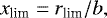
The goal of this section is to estimate the mass of a boson which would be able to describe dark halos of dSph galaxies. For this purpose, we used characteristic quantities of these galaxies: the edge of the galaxy, rlim; the 3D deprojected half-light radius, r1∕2 (i.e. the radius at which luminosity is half total luminosity); the mass M1∕2 enclosed within a sphere of radius r1∕2; the luminosity-weighted average of the square of the line-of-sight velocity dispersion,  ; and errors in M1∕2 and
  . For the stellar component, we assumed constant mass-to-light ratio and used a truncated King profile with a core radius rc calculated from r1∕2 and rlim. For simplicity, star mass contribution to system mass is neglected in any point. Two expressions are used to estimate m from the above quantities. One of themrelates M1∕2 and r1∕2 with M and m. The second one is the virial theorem for the star component which relates rlim and
  to M and m.
5.1 Formulae used to estimate the boson mass
From Eqs. (16) and (14),
 (62)
(62)
and, from Eq. (19),
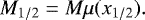 (63)
(63)
Hence,
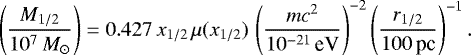 (64)
(64)
In Eq. (64), r1∕2 is expressed in hundreds of parsecs, and M1∕2 in units of 107 M⊙, as those deduced from observations of dSph galaxies (e.g. Wolf et al. 2010, who derived an accurate mass estimator for dispersion-supported stellar systems). In that equation, boson mass appears in units of 10−21 eV in order the numerical coefficient to be close to unity.
ShowingM in the same units that M1∕2, the length scale b reads as
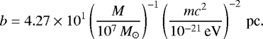 (65)
(65)
Thus, usingEq. (65) in (22), the dimensionless parameter ξ can be expressed as
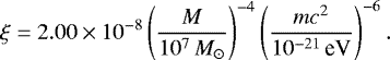 (66)
(66)
Hence, the repulsive effect of the cosmological constant imposes the constraint (from ξ ≤ ξc = 1.65 × 10⁻⁴)
 (67)
(67)
The numerical coefficient in Eq. (67) is five times greater than that derived in Membrado & Pacheco (2012); there, it was imposed that the distance r0 (see Eq. (32)) where the gravitational effect is balanced by the repulsion must be greater than the length scale, b (see Eq. (14)).
Hui et al. (2017) found similar results to those given by Eq. (67) by imposing two different arguments. One argues that dark halo mean density inside half-mass radius must be greater than two hundred times the critical density of the Universe; the other is based on the Jeans length. Within the considerable uncertainties in their results, they give a minimum mass halo of (1–2) × . This bound is 0.3–0.6 times lower than that of Eq. (67). According to this result, the cosmological constant is what actually imposes the lower bound for the mass of these systems.
The virial theorem that we used for the stellar component (assuming spherical symmetry and steady and static conditions) comes from multiplying the radial Jeans equation (see, for example, Binney & Tremaine 1987, p. 198) by 4πr3 and integrating from r = 0 up to r = rlim, where surface terms are neglected. Thus
 (68)
(68)
In Eq. (68), σ is the total velocity dispersion of stars; M(r) is the mass at distance r from the system centre; M⋆, the stellar mass enclosed within a sphere of radius rlim; and, for any quantity Q,
 (69)
(69)
ρ⋆ (r) being stellar mass density at r.
In our study, ρ⋆(r) is approximated by a truncated King profile (King 1962, Eqs. (27) and (29)). Its core radius, rc, is chosen to fulfil
 (70)
(70)
where
![Mathematical equation: \begin{eqnarray}&&F(r) = {1\over z^2}\left[{\cos^{-1}(z)\over z} -(1-z^2)^{1/2}\right], \\ &&z = \left[{1+ (r/r_c)^2\over 1 + (r_{\textrm{lim}}/r_c)^2}\right]^{1/2}. \end{eqnarray}](/articles/aa/full_html/2018/03/aa31447-17/aa31447-17-eq72.png)
For  , we take three times the luminosity-weighted average of the square of the line-of-sight velocity dispersion,
  . Thus, using Eqs. (14), (16), (19) and (18) and the truncated King profile in (68),
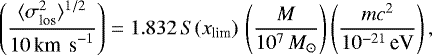 (73)
(73)
where
 (74)
(74)
![Mathematical equation: \begin{equation*} S(x_{\textrm{lim}}) = \left[\int_0^{x_{\textrm{lim}}} F(bx) \mu(x) x \textrm{d}x \over \int_0^{x_{\textrm{lim}}} F(bx) x^2 \textrm{d}x\right]^{1/2}.\end{equation*}](/articles/aa/full_html/2018/03/aa31447-17/aa31447-17-eq77.png) (75)
(75)
In order Eq. (73) to have a numerical coefficient close to unity,  is presented in tens of km s−1.
5.2 Procedure followed to estimate m
Now, let us suppose that we are dealing with Ng galaxies. Then, Nd = 2 Ng is the number of data, and Np = Ng + 1, the number of unknown parameters. In the following, for the galaxy i, we denote data by M1∕2;i and  , and dark halo mass parameter by Mi.
For a particle mass parameter m, we calculated the best-fitting dark halo parameters. Our procedure is as follows:
- 1.
For each galaxy i, numerical values from our model (M) at r1∕2;i of the dark halo mass
![Mathematical equation: $[M_{1/2;\,i}]^{\textrm{M}}$](/articles/aa/full_html/2018/03/aa31447-17/aa31447-17-eq80.png) and of the velocity dispersion
and of the velocity dispersion ![Mathematical equation: $[\langle\sigma_{\textrm{los};\,i}^2\rangle^{1/2}]^{\textrm{M}}$](/articles/aa/full_html/2018/03/aa31447-17/aa31447-17-eq81.png) are calculated from m and Mi: particle mass and dark halo mass fix the length scale bi and ξi from Eqs. (65) and (66), respectively; the dimensionless density profile, ηi(x), is then obtained by solving Eq. (33); this allows us to calculate μi(x1∕2;i) from Eq. (18), with x1∕2;i = r1∕2;i∕bi.
are calculated from m and Mi: particle mass and dark halo mass fix the length scale bi and ξi from Eqs. (65) and (66), respectively; the dimensionless density profile, ηi(x), is then obtained by solving Eq. (33); this allows us to calculate μi(x1∕2;i) from Eq. (18), with x1∕2;i = r1∕2;i∕bi. ![Mathematical equation: $[M_{1/2;\,i}]^{\textrm{M}}$](/articles/aa/full_html/2018/03/aa31447-17/aa31447-17-eq82.png) is then determined from Eq. (64), and
is then determined from Eq. (64), and ![Mathematical equation: $ [\langle\sigma_{\textrm{los};\,i}^2\rangle^{1/2}]^{\textrm{M}} $](/articles/aa/full_html/2018/03/aa31447-17/aa31447-17-eq83.png) from Eq. (73), with xlim;i = rlim;i∕bi.
from Eq. (73), with xlim;i = rlim;i∕bi. - 2.
χ2 is calculated as
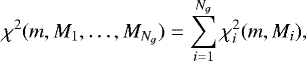 (76)
(76)with
![Mathematical equation: \begin{eqnarray*}\chi^2_i(m,M_i) &=&\left( [M_{1/2;\,i}]^{\textrm{M}} - M_{1/2;\,i} \over \UpDelta^{\pm}_{M_{1/2;\,i}} \right)^2 \nonumber \\&& + \left( [\langle\sigma_{\textrm{los};\,i}^2\rangle^{1/2}]^{\textrm{M}} - \langle\sigma_{\textrm{los};\,i}^2\rangle^{1/2} \over \UpDelta^{\pm}_{\langle\sigma_{\textrm{los};\,i}^2\rangle^{1/2}}\right)^2.\end{eqnarray*}](/articles/aa/full_html/2018/03/aa31447-17/aa31447-17-eq85.png) (77)
(77)For any quantity Q in Eq. (77),
 are errors in Q. If
 ![Mathematical equation: $[Q]^{\textrm{M}} > Q$](/articles/aa/full_html/2018/03/aa31447-17/aa31447-17-eq87.png) ,
,  is taken; otherwise,
  .
. - 3.
The best-fitting dark halo parameters are those which minimize Eq. (76); that is, those which minimize
 given by Eq. (77). We denote the minimum value of
 by
by  , and the dark halo parameter which leads to it by M0;i(m); that is,
 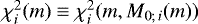 . The minimum value of
  is denoted by χ2(m), which appears for
  ; that is,
  . Thus,
 (78)
(78)The best estimate of m is the particle mass for which χ2(m) takes its minimum value. It happens for m0; that is,
 .
.We can also derive a range of values of m in which there is a 68% chance of finding the true mass in it. This range of values are determined by the condition
 (79)
(79) being solution of
 (80)
(80)(Γ(x) is the Gamma function and γ(x, y), the incomplete gamma function).
5.3 Boson mass estimation from dSph galaxy data
In this work we have dealt with 19 Milky Way (MW) dSph galaxies (eight classical and eleven post-Sloan Digital Sky Survey (SDSS)). Data for r1∕2, rlim, M1∕2,  and errors in M1∕2 and
  have been taken from the work by Wolf et al. (2010). The core radius, rc, of the truncated King profile for the stellar component of each galaxy is obtained by imposing Eq. (70).
In Fig. 4, we show χ2(m)∕(Nd − Np) obtained from data of the eight classical MW dSph, and that obtained from including those of eleven post-SDSS MW dSph as well. In both cases, the minimum of χ2 appears for m0c2 = 3.5 × 10⁻²² eV. In the first case,  , while in the second case,
  . This value m0 is in agreement with the result by Hui et al. (2017) who state that the most significant observational consequences occur if the candidate mass is in the range 1–10 ×10−22 eV.
This estimation of m0 used in Eq. (67) leads to the lower bound (LB) for the dark halo mass
 (81)
(81)
The model for m = m0 and M = MLB presents a length scale b = 0.69 kpc. The classical turning point is found at x1 = 13.9, that is, at r1 = 9.6 kpc, containing 79% total dark halo mass, M(r1) = 4.0 × 10⁶ M⊙. The sphere containing 99% halo mass has a dimensionless radius x99 = 30.6, which represents r99 = 21.1 kpc. The dark halo ends at x2 = 42.7; that is r2 = 29.4 kpc. It should be expected that such large halo would suffer tidal effects in the Milky Way group, but it could be found as an isolated galaxy in regions far away from large galaxies.
For Ng = 8,  ; then, applying Eq. (79) to the results shown in Fig. 4 from classical dSph,
  eV. When post-SDSS dSph are also considered, Ng = 19 and
  ; so, Eq. (79) together with Fig. 4 lead to
  eV. Differences between both mass ranges appear to be due to the large errors in M1∕2 given by Wolf et al. (2010) for the post-SDSS MW dSph galaxies. We could say that the data from the classical dSph are those which roughly set the best estimate of m; when more dSph data with larger errors are adding, the estimate does not significantly change but errors increase. In this sense, we note that when the χ2 fit is only done with eleven post-SDSS dSph, the best estimate is m0c2 = 1.7 × 10⁻²¹ eV, with
  , but the range of values of m with a 68% chance of finding the true mass extends up to m0c2 = 2 × 10⁻²³ eV (for m0c2 = 3.5 × 10⁻²² eV, χ2 ∕10 = 6.6∕10).
We should also say that Lyman-α forest, favours mc2 ≥ 10–20 ×10−22 eV, though it is discussed in the literature whether more sophisticated models of recognization could go in favour of smaller masses (Hui et al. 2017). Nevertheless, it must be borne in mind that these bounds are not derived from FDM simulations; they come from CDM simulations in which a cut-off in the linear power spectrum would account for quantum effects. To derive reliable bounds for Lyman-α forest, it would require a self-consistent fuzzy dark matter simulations.
In Table 4, we show several quantities obtained from the model that minimize χ2, for the galaxies treated in this work. From this table:
- 1.
All dSph galaxies present ξ ≪ ξc. Hence, the cosmological constant does not affect to the structure of their dark haloes. It should be noticed that though dark halo masses are between nine and twenty times the lower bound given by Eq. (81), a factor 10 in M applied to Eq. (66) makes ξ to decrease 104 times.
- 2.
Dark halo masses, M0, that minimize χ2 range from 4.7 × 10⁷ M⊙ (Hercules) up to 1.1 × 10⁸ M⊙ (Willman I). As one notes, there is only a factor of 2.3 between these two masses.
- 3.
With respect to length scale b, it ranges from 31.1 pc (Willman I) up to 74.8 pc (Hercules).
- 4.
It is actually surprising that the ultra-faint dSph galaxies Segue I and Willman I show the more massive dark haloes. But we note that there is no relation between galaxy luminosity and dark halo mass. In fact, although there are not great differences between dark haloes of the dSph galaxies treated (as much, a factor of 2.4 in mass or length scale), the stellar component differs appreciably from one to another galaxy.
- 5.
Galaxies present great differences with respect to values of the dimensionless half-light radius, r1∕2∕b, and the dimensionless limit radius of galaxy luminosity, rlim∕b (and hence, with respect to the dimensionless core radius, rc∕b (see Eq. (70)).
- 6.
There are five dSph galaxies with r1∕2∕b much smaller than the dimensionless classical turning point of the dark component, x1 = 11.9 (Willman, Segue I, Canes Ventici II, Leo IV and Coma Berenices show r1∕2∕b < 2.2). And, only three galaxies show r1∕2∕b > x1 (Ursa Minor, Sextans and Formax that shows r1∕2∕b = 21). The mean value of r1∕2∕b is 6.2, close to half x1.
- 7.
For seven galaxies, their edge of luminosity does not reach x1 (Willman, Segue I, Coma Berenices, Canes Ventici II, Ursa Major II, Leo IV and Leo II). However, there are other five (Sculptor, Ursa Minor, Canes Venatici I, Sextans and Fornax) that have it further than the sphere containing 99% dark halo mass, x99 = 19.9 (Membrado et al. 1989). In any case, the mean value of rlim∕b is close to that value, ⟨rlim∕b⟩ = 21.9.
- 8.
The quotient M1∕2∕M0 gives the percentage of dark halo mass up to half-light radius, r1∕2. It presents great differences among the galaxies studied. They range from 0.3% for Willman I up to 99.4% for Fornax, showing a mean value of 31.1%.
- 9.
Mass-to-light ratios also differ appreciably (for luminosity values, L, see Wolf et al. 2010). At half-light radius, the quotient M1∕2∕(L∕2), ranges from 9.0 (Fornax) up to 3140 (Ursa major II), with ⟨M1∕2∕(L∕2)⟩ = 712.7.
- 10.
With respect to values of M1∕2 and
 derived from the model minimizing χ2, we can see that they are in agreement with data presented by Wolf et al. (2010), except for two dSph galaxies. Sculptor exceeds 12% in M1∕2 while the upper error represents 7%; and Sextans, 24% and 16%, respectively. Sculptor is also 3% down in
  while error is 2%.
Now, we could estimate tidal force effects exerted by the Milky Way group on dSph galaxies. A rough estimation of a tidal radius, rT, can be derived from the equation (see e.g. Membrado & Pacheco 2013)
![Mathematical equation: \begin{eqnarray*} && \left[{G M_{\textrm{MW}}[R] \over R^2} - {\UpLambda c^2 R \over 3}\right]+ \left[{GM_{DS}[r_T]\over r^2_T} - {\UpLambda c^2 r_T \over 3}\right] \nonumber \\ &&\quad \approx \left[{GM_{\textrm{MW}}[R - r_T] \over (R - r_T)^2} - {\UpLambda c^2 (R - r_T) \over 3}\right].\end{eqnarray*}](/articles/aa/full_html/2018/03/aa31447-17/aa31447-17-eq114.png) (82)
(82)
This equation is the balance of strengths per unit mass in the direction that joins the centres of the dSph and the MW. The first term in brackets on the left hand side denotes the rotation of the dSph around the MW; MMW[R] stands for the mass of the MW group at a distance R (dark halo and galaxy masses are included) where the dSph galaxy is located. The other terms in brackets are gravitational strengths per unit mass due: (1) to the dSph mass up to rT, MDS[rT], and to the cosmological constant at a distance rT from the centre of the dSph; and (2) to the MW group mass and to the cosmological constant at a distance R − rT from the centre of the MW.
For the mass of the Milky Way group as a function of the distance from the MW centre, we have used that proposed by Membrado & Pacheco (2016):
![Mathematical equation: \begin{equation*}M_{\textrm{MW}}[R] = M_{\textrm{MW}}[R_s]\left(R/R_s\right)^{p}, \end{equation*}](/articles/aa/full_html/2018/03/aa31447-17/aa31447-17-eq115.png) (83)
(83)
with Rs = 514 kpc, p = 0.631, and MMW[Rs] = 3.8 × 10¹¹ M⊙. In Membrado & Pacheco (2016), we proposed two equations (discrete model) containing surface terms to estimate galaxy sample masses. When the surface terms are neglected, these equations provide the so-called virial and projected masses. In that work, the galaxies studied by Karachentsev (2005) were used. The parameters for MMW[R] were chosen to reproduce the harmonic radius of the Milky Way group and the mean separation between galaxies and the MW, derived from the discrete model (199 kpc and 214 kpc, respectively).
We haveestimated rT for the eight classical dSph. The distances to those galaxies given by Karachentsev (2005) have been used. For their masses, we use Eq. (19), that is MDS[r] = M0 μ(r∕b), with the M0’s presented in Table 4. We have seen that for the classical dSph galaxies, rT ∕b ranges from 75.4 (Sextans) up to 236.8 (Leo I). These dimensionless distances are beyond the dimensionless distance enclosing 99% of the mass (x99 = 19.9). From these results, we conclude that tidal effects on the eight classical dSph galaxies would be negligible.
It can also be estimated the mass, Mm[R], of a dSph galaxy that orbiting around the MW and located at a distance R fulfils rT = r99. DSph galaxies with masses smaller than Mm[R] could suffer disruption by tidal forces. A value for its crossing time can be obtained by
![Mathematical equation: \begin{equation*}t_{\textrm{cross}} [R]\approx R\,\left[{G M_{\textrm{MW}}[R] \over R} - {\UpLambda c^2 R^2\over 3}\right]^{-1/2}. \end{equation*}](/articles/aa/full_html/2018/03/aa31447-17/aa31447-17-eq116.png) (84)
(84)
As examples: Mm[200 kpc] = 1.07 × 10⁷ M⊙, H0 tcross[200 kpc] = 0.22, where H0 is the Hubble function at present; Mm[400 kpc] = 7.4 × 10⁶ M⊙, H0 tcross[400 kpc] = 0.53. Hence, a dSph with the lower limit mass, MLB = 5.1 × 10⁶ M⊙, could not be orbiting around the MW. If these galaxies exist, they should be isolated, far away from any massive galaxy.
We have also compared cosmological constant contributions to the gravitational force in the host halo and in the classical dSph galaxies. In the dark halo of the Milky Way group, the nearest dSph galaxy, Ursa Minor, is located at 63 kpc, while the farthest one, Leo I, is found at 250 kpc. At these distances, the repulsive contributions represent 0.4% and 5.5% the attractive contributions. At the tidal radii of Ursa Minor (4.9 kpc) and of Leo I (13.6 kpc), Λ contribution represents 0.1% and 3.5% the mass contribution to the gravitational strength. Hence, it could be said that for the classical dSph galaxies, repulsive to attractive forces ratio is even a bit smaller at their tidal radii than at their locations in the Milky Way Group halo.
As has been seen, MW dSph galaxies show different luminosity component profiles which do not depend on dark halo mass. Despite this variety, by simplicity, we could address our attention to a profile family leading to the same M1∕2∕M, M1∕2∕(L∕2) and rlim ∕b, in order to see how the luminosity component changes for different ξ. We have chosen their mean values from the sample of MW dSph galaxies; that is, M1∕2∕M = 0.311, M1∕2∕(L∕2) = 713 and rlim ∕b = 21.9. Results are presented in Table 5.
The quantities shown in Table 5 are derived as follows. After assuming m = 3.5 × 10⁻²² eV, Eq. (66) gives the dark halo mass, M, for each ξ; then, Eq. (65) provides the length scale b. The value chosen for M1∕2∕M, allows us to fix M1∕2. The use of Eq. (63), together with (18), the dimensionless densities η given in Fig. 3, and Eq. (16) determine r1∕2. The edge of the luminosity, rlim comes from assuming the value of rlim∕b. The core radius rc is calculated from Eq. (70). The velocity dispersion  is then obtained using Eq. (73). Finally, luminosity comes from assuming the value of M1∕2∕(L∕2). The radius enclosing 99% of the dark halo mass, r99, is also presented in this table.
From this table, we can see that, from ξ = 10−6 up to ξc, the edge of the luminosity component, rlim, ranges from 4 to 15 kpc. This large values, together with small numbers of stars, would make the identification of dSph galaxy members difficult.
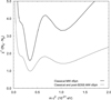 |
Fig. 4 Normalized χ2 from the eight classical MW dSph, and from 19 dSph galaxies which include the classical and the post-SDSS MW dSph, as a function of the boson mass, m. |
Several quantities derived from the model which minimizes χ2 for classical (upper panel) and post-SDSS MW dSph galaxies (bottom panel).
Several quantities of dark and luminosity components for different ξ.
6 Conclusions
- 1.
We have included dark energy of the cosmological background in the structure of a cluster composed by self-gravitating collisionless Newtonian bosons. Dark energy is assumed to be the cosmological constant, and bosons are treated in their ground state. The structure of the system is derived by solving a variational problem in the particle number density. The model is used to describe dark haloes of dSph galaxies, and is tested in 19 Milky Way dSph galaxies.
- 2.
The magnitude of the effects of the cosmological constant on the structure of these systems only depends on the value of one parameter. This parameter, ξ, is the quotient between two gravitational force scales: one, repulsive, due to the cosmological constant, and the another, attractive, due to matter.
- 3.
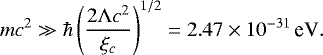
The influence of the cosmological constant on bound structures is only appreciable for 10−5 < ξ ≤ ξc = 1.65 × 10⁻⁴. For ξ > ξc, bound assemblies can not be created due to the repulsion exerted by the cosmological constant. Hence, ξc imposes a lower bound for the system mass which is function of the particle mass. This lower limit is approximately five times greater than that estimated by us in Membrado & Pacheco (2012), where a more simple argument were used. From ξc, it is also derived that assemblies are Newtonian if the particle mass is much greater than 2.5 × 10⁻³¹ eV.
- 4.
The solution for ξ = 0 has a classical turning point where the kinetic energy per particle is null. However, when 0 < ξ ≤ ξc, the cosmological constant makes the kinetic energy to have a second zero beyond the classical turning point. This means that there is tunnelling through a potential barrier. We have estimated the mean life of these systems, concluding that their existence is not affected by the age of the Universe.
- 5.
We have developed the virial theorem for these systems to check the solutions of the variational problem. We have found that the energy of the system is not a third of the product of the energy per particle and the number of particles, as happens when cosmological constant is neglected: now, four thirds of the potential energy due to the cosmological constant must be added.
- 6.
The model is tested by using four characteristic data from 19 Milky Way dSph galaxies (eight classical and eleven post-Sloan Digital Sky Survey), taken from the work by Wolf et al. (2010): galaxy radius, rlim; 3D deprojected half-light radius, r1∕2; luminosity-weighted averages of the square of line-of-sight velocity dispersions,
 ; and mass M1∕2 enclosed up to r1∕2. Mass distribution from our model allows us to relate r1∕2 and M1∕2 with the halo total mass, M, and the particle mass, m; and, the virial theorem for the stellar component, rlim and
  with M and m. The stellar component is approximated by a truncated King profile.
 - 7.
We have calculated χ2 taking into account errors in M1∕2 and in
 . From χ2, we find that when classical dSph are considered, the range of values of m in which there is a 68% chance of finding the true mass, is
  eV. These values are in the range 1–10 ×10−22 eV proposed by Hui et al. (2017) if the dark matter is composed by fuzzy dark matter (ultralight bosons). When post-SDSS galaxies are included,
  eV are obtained. We should say that discrepancies between both ranges are due to large M1∕2 errors inpost-SDSS dwarfs.
 - 8.
The best estimate of particle mass, m0 = 3.5 × 10⁻²² eV, leads to a lower limit for bound dark haloes of MLB = 5.1 × 10⁶ M⊙. Hui et al. (2017) have also derived a lower bound, but based on arguments about the mass density at half-light radius (greater than two hundred times the critical density) and on the Jeans length; within the considerable uncertainties and assuming m0, their value would be about 1.5–3 ×10⁶ M⊙. These results would make us conclude that the repulsion of the cosmological constant could impose the minimum mass for these dark haloes. In our calculations, surface terms of the virial theorem at x2 are null; that is, quantum pressure at x2 is zero. This is due to the fact that at x2, n′ = n″ = 0. This result is for isolated dSph galaxies and without taking into account their environments. Nevertheless, it should be said that simulations indicate that quantum pressure would affect the survivability of the smallest halos (see, for example: Mocz et al. 2017). Hence, the minimum mass of dSph galaxies would be also limited by quantum pressure.
- 9.
The 19 dSph galaxies show values of ξ from 1.6 × 10⁻⁸ (Carina) up to from 6.9 × 10⁻¹⁰ (Willman I). This means that the cosmological constant effects are negligible in the structure of these galaxies. However, their total halo masses range from 4.7 × 10⁷ M⊙ (Hercules) up to 1.1 × 10⁸ M⊙ (Willman I); that is ~10–20 times the lower bound for dark halo masses. This is because ξ α M−4. The influence of the cosmological constant begins to be relevant for dark halo masses smaller than 107 M⊙ (ξ > 10−5) up to the lower limit imposed by the cosmological constant repulsion (5.1 × 10⁶ M⊙). However, we note once again that for these low halo masses there are other mechanisms that could dominate over the dark energy repulsion regarding the disruption of halos, such as quantum pressure or dynamical friction. In this respect, we have estimated that the minimun mass of a dSph galaxy in the Milky Way group that does not suffer tidal effects would be about 7 × 10⁶ M⊙. Less massive dSph galaxies would have to be isolated, and far away from any massive galaxy.
- 10.
Assuming M∕M1∕2 = 0.311, M1∕2∕(L∕2) = 713, and rlim∕b = 21.9, corresponding to mean values of those quantities from the 19 galaxies, 10−5 < ξ ≤ ξc dark haloes would contain stellar components inside ~8–15 kpc with luminosities ~9–4 ×10³ L⊙. With these characteristics, their detection could be rather difficult.
Appendix A: The variational problem
We are dealing with a variational problem of the kind given by Eq. (7); that is, with
![Mathematical equation: \begin{equation*}\int_0^R \delta F[n] \textrm{d}r = 0, \end{equation*}](/articles/aa/full_html/2018/03/aa31447-17/aa31447-17-eq123.png) (A.1)
(A.1)
where  , and R, the radius of the system. Assuming a profile for n(r), we increase a quantity δn(r). Thus,

Hence, at each point, F[n] will be modified by an amount δF[n] given by
 (A.5)
(A.5)
And, taking into account that

Eq. (A.5) reads as
![Mathematical equation: \begin{eqnarray*} \delta F &=& \delta n \left[ {\partial F\over \partial n} - {\textrm{d}\over {\textrm{d}} r}\left(\partial F\over \partial \dot n\right) + {\textrm{d}^2\over {\textrm{d}} r^2}\left(\partial F\over \partial \ddot n\right) \right] \nonumber \\ && + {\textrm{d}\over {\textrm{d}}r}\left\{ \delta n \left[{\partial F\over \partial\dot n} - {\textrm{d}\over {\textrm{d}}r}\left({\partial F\over \partial\ddot n}\right)\right] + {\textrm{d} \delta n \over {\textrm{d}}r} \left[{\partial F\over \partial \ddot n}\right] \right\}.\end{eqnarray*}](/articles/aa/full_html/2018/03/aa31447-17/aa31447-17-eq128.png) (A.8)
(A.8)
Thus, using Eq. (A.8) in Eq. (A.1), and assuming δn(0) = δn(R) = 0, and δṅ (0) = δṅ(R) = 0, the condition
 (A.9)
(A.9)
must be fulfilled at any point.
Appendix B: Kinetic contribution to the virial theorem
The first term of Eq. (45), which we call T1, can be expressed as
![Mathematical equation: \begin{equation*}T_1 = 4\pi \int_0^R r^3 n {\textrm{d} \over {\textrm{d}}r}\left[{n r^2 e_{\textrm{kin}}\over n r^2}\right] \textrm{d}r. \end{equation*}](/articles/aa/full_html/2018/03/aa31447-17/aa31447-17-eq130.png) (B.1)
(B.1)
Hence,
![Mathematical equation: \begin{equation*}{T_1} = 4 \pi\int_0^R \left[ r {\textrm{d} ( n r^2 e_{\textrm{kin}}) \over {\textrm{d}}r} - r^3 e_{\textrm{kin}} {\textrm{d} n\over {\textrm{d}}r} - 2 n r^2 e_{\textrm{kin}} \right] \textrm{d}r,\end{equation*}](/articles/aa/full_html/2018/03/aa31447-17/aa31447-17-eq131.png) (B.2)
(B.2)
and using the expression of ekin given by Eq. (9) in the first and second term of the integral (B.2),
![Mathematical equation: \begin{equation*}{T_1} = 4\pi \left\{-{\hbar^2\over 4 m}\left[ r^2 \dot n + r^3 \ddot n - r^3 {\dot n^2\over n} \right]_0^R -2\int_0^R n r^2 e_{\textrm{kin}} \textrm{d}r \right\}. \end{equation*}](/articles/aa/full_html/2018/03/aa31447-17/aa31447-17-eq132.png) (B.3)
(B.3)
The first term on the right hand side of Eq. (B.3) is a surface term. When ṅ (R) = 0 and  ,
,
 (B.4)
(B.4)
T being the kinetic energy of the system.
References
- Amendola, L., & Barbieri, R. 2006, Phys. Lett. B, 642, 192 [NASA ADS] [CrossRef] [Google Scholar]
- Basdevant, J. L., Martin, A., & Richard, J. M. 1990, Nucl. Phys. B, 343, 60 [NASA ADS] [CrossRef] [Google Scholar]
- Binney, J., & Tremaine, S. 1987, Galactic Dynamics (Princeton: Princeton Univ. Press) [Google Scholar]
- Bovill, M. S., & Ricotti, M. 2009, ApJ, 693, 1859 [NASA ADS] [CrossRef] [Google Scholar]
- Burkert, A. 1995, ApJ, 447, L25 [NASA ADS] [CrossRef] [Google Scholar]
- Calabrese, E., & Spergel, D. N. 2016, MNRAS, 460, 4397 [NASA ADS] [CrossRef] [Google Scholar]
- Chavanis, P.-H. 2011, Phys. Rev. D, 84, 043531 [NASA ADS] [CrossRef] [Google Scholar]
- Chen, S.-R., Schive, H.-Y., & Chiueh, T. 2017, MNRAS, 468, 1338 [NASA ADS] [CrossRef] [Google Scholar]
- de Blok, W. J. G. 2005, ApJ, 634, 227 [NASA ADS] [CrossRef] [Google Scholar]
- de Blok, W. J. G., & Bosma, A. 2002, A&A, 385, 816 [NASA ADS] [CrossRef] [EDP Sciences] [Google Scholar]
- Diemand, J., Kuhlen, M., & Madau, P. 2007, ApJ, 667, 859 [NASA ADS] [CrossRef] [Google Scholar]
- Gentile, G., Burkert, A., Salucci, P., Klein, U., & Walter, F. 2005, ApJ, 634, L145 [NASA ADS] [CrossRef] [Google Scholar]
- Gilmore, G., Wilkinson, M. I., Wyse, R. F. G., et al. 2007, ApJ, 663, 948 [NASA ADS] [CrossRef] [Google Scholar]
- Giocoli, C., Tormen, G., & van den Bosch, F. C. 2008, MNRAS, 386, 2135 [NASA ADS] [CrossRef] [Google Scholar]
- Griffin, A., Snoke, D. W., & Stringari, S. 1996, Bose–Einstein Condensation (Cambridge University Press) [Google Scholar]
- Hu, W., Barkana, R., & Gruzinov, A. 2000, Phys. Rev. Lett., 85, 1158 [NASA ADS] [CrossRef] [PubMed] [Google Scholar]
- Hui, L., Ostriker, J. P., Tremaine, S., & Witten, E. 2017, Phys. Rev. D, 95, 043541 [NASA ADS] [CrossRef] [PubMed] [Google Scholar]
- Jetzer, P. 1992, Phys. Rep., 220, 163 [NASA ADS] [CrossRef] [Google Scholar]
- Karachentsev, I. D. 2005, AJ, 129, 178 [NASA ADS] [CrossRef] [Google Scholar]
- Karachentsev, I. D., Makarova, L. N., Makarov, D. I., Tully, R. B., & Rizzi, L. 2015, MNRAS, 447, L85 [NASA ADS] [CrossRef] [Google Scholar]
- Kauffmann, G., White, S. D. M., & Guiderdoni, B. 1993, MNRAS, 264, 201 [NASA ADS] [CrossRef] [Google Scholar]
- Kazantzidis, S., Mayer, L., Mastropietro, C., et al. 2004, ApJ, 608, 663 [NASA ADS] [CrossRef] [Google Scholar]
- King, I. 1962, AJ, 67, 471 [NASA ADS] [CrossRef] [Google Scholar]
- Klypin, A., Kravtsov, A. V., Valenzuela, O., & Prada, F. 1999, ApJ, 522, 82 [Google Scholar]
- Lee, J.-W., & Koh, I.-G. 1996, Phys. Rev. D, 53, 2236 [NASA ADS] [CrossRef] [Google Scholar]
- Lévy-Leblond, J.-M. 1969, J. Math. Phys., 10, 806 [NASA ADS] [CrossRef] [Google Scholar]
- Lieb, E. H., & Seiringer, R. 2009, The Stability of Matter in Quantum Mechanics (Cambridge University Press) [Google Scholar]
- Makarov, D., Makarova, L., Sharina, M., et al. 2012, MNRAS, 425, 709 [NASA ADS] [CrossRef] [Google Scholar]
- Marsh, D. J. E. 2016, Phys. Rep., 643, 1 [NASA ADS] [CrossRef] [Google Scholar]
- Martinez, G. D., Minor, Q. E., Bullock, J., et al. 2011, ApJ, 738, 55 [NASA ADS] [CrossRef] [Google Scholar]
- Matos, T., & Arturo Ureña-López, L. 2001, Phys. Rev. D, 63, 063506 [NASA ADS] [CrossRef] [Google Scholar]
- Matos, T., & Ureña-López, L. A. 2000, Classical and Quantum Gravity, 17,L75 [NASA ADS] [CrossRef] [Google Scholar]
- Matthews, P. T. 1963, Introduction to Quantum Mechanics (McGraw-Hill), International Series in Pure and Applied Physics [Google Scholar]
- Membrado, M., & Pacheco, A. F. 2012, Europhys. Lett., 100, 39004 [NASA ADS] [CrossRef] [Google Scholar]
- Membrado, M., & Pacheco, A. F. 2013, A&A, 551, A68 [NASA ADS] [CrossRef] [EDP Sciences] [Google Scholar]
- Membrado, M., & Pacheco, A. F. 2016, A&A, 590, A58 [NASA ADS] [CrossRef] [EDP Sciences] [Google Scholar]
- Membrado, M., Pacheco, A. F., & Sañudo, J. 1989, Phys. Rev. A, 39, 4207 [NASA ADS] [CrossRef] [PubMed] [Google Scholar]
- Mocz, P., Vogelsberger, M., Robles, V. H., et al. 2017, MNRAS, 471, 4559 [NASA ADS] [CrossRef] [Google Scholar]
- Moore, B., Ghigna, S., Governato, F., et al. 1999, ApJ, 524, L19 [Google Scholar]
- Navarro, J. F., Frenk, C. S., & White, S. D. M. 1997, ApJ, 490, 493 [NASA ADS] [CrossRef] [Google Scholar]
- Navarro, J. F., Hayashi, E., Power, C., et al. 2004, MNRAS, 349, 1039 [NASA ADS] [CrossRef] [Google Scholar]
- Ricotti, M., & Gnedin, N. Y. 2005, ApJ, 629, 259 [NASA ADS] [CrossRef] [Google Scholar]
- Ruffini, R., & Bonazzola, S. 1969, Phys. Rev., 187, 1767 [NASA ADS] [CrossRef] [Google Scholar]
- Sahni, V., & Wang, L. 2000, Phys. Rev. D, 62, 103517 [NASA ADS] [CrossRef] [MathSciNet] [Google Scholar]
- Schive, H.-Y., Chiueh, T., & Broadhurst, T. 2014, Nat. Phys., 10, 496 [CrossRef] [Google Scholar]
- Simon, J. D., Geha, M., Minor, Q. E., et al. 2011, ApJ, 733, 46 [NASA ADS] [CrossRef] [Google Scholar]
- Spergel, D. N., Verde, L., Peiris, H. V., et al. 2003, ApJS, 148, 175 [NASA ADS] [CrossRef] [Google Scholar]
- Springel, V., Wang, J., Vogelsberger, M., et al. 2008, MNRAS, 391, 1685 [NASA ADS] [CrossRef] [Google Scholar]
- Suárez, A., Robles, V. H., & Matos, T. 2014, in Accelerated Cosmic Expansion, eds. C. Moreno González, J. E. Madriz Aguilar, & L. M. Reyes Barrera, Astrophysics and Space Science Proceedings, 38, 107 [NASA ADS] [CrossRef] [Google Scholar]
- Tikhonov, A. V., & Klypin, A. 2009, MNRAS, 395, 1915 [NASA ADS] [CrossRef] [MathSciNet] [Google Scholar]
- Weinberg, D. H., Bullock, J. S., Governato, F., Kuzio de Naray, R., & Peter, A. H. G. 2015, Proc. Natl. Acad. Sci., 112, 12249 [Google Scholar]
- Wolf, J., Martinez, G. D., Bullock, J. S., et al. 2010, MNRAS, 406, 1220 [NASA ADS] [Google Scholar]
All Tables
Dimensionless quantities appearing in the virial theorem and in the energy of a boson cluster.
Several quantities derived from the model which minimizes χ2 for classical (upper panel) and post-SDSS MW dSph galaxies (bottom panel).
All Figures
|
Fig. 1 For ξ = 0, gravitational energy, νM and single-particle energy, ϵ, as a functionof the dimensionless distance x. The classicalturning point x1 is marked. |
| In the text | |
|
Fig. 2 Choice of a0 for different values of ξ (see text). |
| In the text | |
|
Fig. 3 Left panels: dimensionless particle number density, η, as a functionof x, for three values of ξ. The bottom panel corresponds to the critical value ξc. Right panels: dimensionless energies per particle for the same values of ξ shown in left panels (gravitational energy due to matter, νM; total gravitational energy, νM + νΛ; single-particle energy, ϵ), as a functionof the dimensionless distance x. The distances x1, x0 and x2 for ξc are marked in the bottom right panel. |
| In the text | |
|
Fig. 4 Normalized χ2 from the eight classical MW dSph, and from 19 dSph galaxies which include the classical and the post-SDSS MW dSph, as a function of the boson mass, m. |
| In the text | |
Current usage metrics show cumulative count of Article Views (full-text article views including HTML views, PDF and ePub downloads, according to the available data) and Abstracts Views on Vision4Press platform.
Data correspond to usage on the plateform after 2015. The current usage metrics is available 48-96 hours after online publication and is updated daily on week days.
Initial download of the metrics may take a while.