| Issue |
A&A
Volume 610, February 2018
|
|
|---|---|---|
| Article Number | L2 | |
| Number of page(s) | 4 | |
| Section | Letters to the Editor | |
| DOI | https://doi.org/10.1051/0004-6361/201732262 | |
| Published online | 14 February 2018 | |
Letter to the Editor
Discovery of 105 Hz coherent pulsations in the ultracompact binary IGR J16597–3704
1
Dipartimento di Fisica, Università degli Studi di Cagliari,
SP Monserrato-Sestu km 0.7,
09042
Monserrato, Italy
e-mail: This email address is being protected from spambots. You need JavaScript enabled to view it.
2
Department of Physics and Astronomy, Michigan State University,
East Lansing,
MI, USA
3
ISDC, Department of Astronomy, University of Geneva,
Chemin d’Écogia 16,
1290
Versoix, Switzerland
4
University of Alberta, Physics Dept.,
CCIS 4-181,
Edmonton
AB T6G 2E1, Canada
5
Physics and Astronomy, University of Southampton,
Southampton,
Hampshire
SO17 1BJ, UK
6
Anton Pannekoek Institute for Astronomy, University of Amsterdam,
Science Park 904,
1098 XH,
Amsterdam, The Netherlands
7
Department of Physics, Box 41051, Science Building, Texas Tech University,
Lubbock,
TX
79409-1051, USA
8
Università degli Studi di Palermo, Dipartimento di Fisica e Chimica,
via Archirafi 36,
90123
Palermo, Italy
9
INAF, Osservatorio Astronomico di Cagliari,
Via della Scienza 5,
09047
Selargius, CA, Italy
10
INAF, Osservatorio Astronomico di Roma,
Via di Frascati 33,
00044
Monteporzio Catone, Roma, Italy
Received:
8
November
2017
Accepted:
28
November
2017
Abstract
We report the discovery of X-ray pulsations at 105.2 Hz (9.5 ms) from the transient X-ray binary IGR J16597–3704 using NuSTAR and Swift. The source was discovered by INTEGRAL in the globular cluster NGC 6256 at a distance of 9.1 kpc. The X-ray pulsations show a clear Doppler modulation that implies an orbital period of ~46 min and a projected semi-major axis of ~5 lt-ms, which makes IGR J16597–3704 an ultracompact X-ray binary system. We estimated a minimum companion mass of 6.5 × 10⁻¹⁰ M⊙, assuming a neutron star mass of 1.4 M⊙, and an inclination angle of <75° (suggested by the absence of eclipses or dips in its light curve). The broad-band energy spectrum of the source is well described by a disk blackbody component (kT ~ 1.4 keV) plus a comptonised power-law with photon index ~2.3 and an electron temperature of ~30 keV. Radio pulsations from the source were unsuccessfully searched for with the Parkes Observatory.
Key words: binaries: general / stars: neutron / X-rays: binaries / accretion, accretion disks
© ESO, 2018
1 Introduction
So far, 19 accreting millisecond X-ray pulsars (AMXP) were discovered in low-mass X-ray binaries, with spin periods ranging from 1.7 to 6.1 ms (e.g. Burderi & Di Salvo 2013; Patruno et al. 2017). The short periods of these sources are the result of the long-lasting mass transfer from the companion star through Roche-lobe overflow (Alpar et al. 1982), a scenario that was observationally confirmed by the discovery of transitional binary pulsars (see Papitto et al. 2013, and references therein). Almost a third of the total sample of AMXPs is classified as ultracompact binary systems, which have extremely short orbital periods (Porb < 1 h; Galloway et al. 2002; Markwardt et al. 2002; Kirsch et al. 2004; Krimm et al. 2007; Altamirano et al. 2010; Sanna et al. 2017b). The rest of the sample have Porb < 12 h, except for Aql X–1 (Porb ~ 19 h; Welsh et al. 2000). The distribution of short orbital periods suggests that typical AMXP companion star have masses below 0.2 M⊙ (Patruno & Watts 2012).
We report here on the discovery of millisecond X-ray pulsations from IGR J16597–3704, a transient source discovered by INTEGRAL on 2017 October 21 (Bozzo et al. 2017a) that is localised within the globular cluster NCG 6256 at 9.1 kpc (Bozzo et al. 2017b; Valenti et al. 2007). The best-known position of the source is at RA = 16h59m32.9007s ± 0.0021s, Dec = −37°07′14.22′′± 0.18′′ (Tetarenko et al. 2017).
2 Observations and data reduction
2.1 NuSTAR
NuSTAR (Harrison et al. 2013) observed IGR J16597–3704 (Obs.ID. 90301324001) on 2017 October 26 at 12:16 UTC for an elapsed time of ~84 ks, corresponding to a total exposure of ~42 ks. We performed standard screening and filtering of the events using the NuSTAR data analysis software (NUSTARDAS) version 1.5.1. We extracted source events from the two focal plane modules (FMPA and FMPB) within a circular region of radius 100″ for the light curve and 60″ for the spectrum, centred on the source position. Similar regions, but located away from the source, were used to extract the background products. Response files were generated using the NUPRODUCTS pipeline, and the photon arrival times were barycentre-corrected by using the BARYCORR tool. No Type I bursts were recorded during the observation.
2.2 INTEGRAL
We considered all the public available INTEGRAL science windows for IBIS/ISGRI (20–100 keV, Lebrun et al. 2003; Ubertini et al. 2003) that were performed in the direction of IGR J16597–3704 during the outburst (i.e. revolutions 1876 and 1878, covering from 2017 October 21 at 04:40 to October 27 at 14:51, UTC). During this period, the source was not detected by JEM-X (Lund et al. 2003) because of the large off-axis position (Bozzo et al. 2017a). All the INTEGRAL public data were analysed using version 10.2 of the OSA software (Courvoisier et al. 2003). IGR J16597–3704 was detected in the total IBIS/ISGRI 20–40 keV mosaic at 10 σ. We extracted a single ISGRI spectrum using the entire available exposure time (53 ks).
2.3 Swift
We used one Swift/XRT (Gehrels et al. 2004) observation of IGR J16597–3704 taken on 2017 October 25 at 07:51 (UTC) in WT mode (1 ks). We processed the XRT data with XRTPIPELINE version 0.13.4, extracted source and background spectra using XSELECT, and produced an ancillary response file for the spectrum with XRTMKARF. We used circular extraction regions with radii of 20 pixels (~47″) for both the source and background, considering only grade 0events to avoid low-energy calibration issues.
2.4 Radio observations with Parkes
IGR J16597–3704 was observed for 2.9 h on 2017 November 3 at the Parkes radio telescope with the aim of searching for radio pulsations. The data were collected using the BPSR backend over a bandwidth of 400 MHz (reduced to 315 after interference removal) centred at 1382 MHz and split into 1024 frequency channels. The signal was two-bit sampled every 64 μs. Data were folded using the X-ray ephemeris of Table 1 and searched over dispersion measures DM < 700 pc cm–3 (the nominal DM expected for NGC 6256 ranges from 250 to 450 pc cm–3; Taylor & Cordes 1993; Cordes & Lazio 2002; Schnitzeler 2012; Yao et al. 2017). Data were also folded with different trial values in TNOD, while the uncertainty on the other parameters was neglected as it would affect the width of the folded profile by <10%. No radio pulsation were found down to a flux density of 0.05 mJy.
Orbital parameters and spin frequency of IGR J16597–3704 estimated from the NuSTAR data without a frequency derivative (left) and including a frequency derivative (right).
3 Data analysis
3.1 Timing analysis
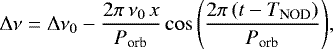
To search for coherent signals, we extracted a power density spectrum (PDS) from the NuSTAR observation by averaging together nine power spectra produced over 4096 s of data (Fig. 1). The PDS shows a highly significant (>100 σ) broad double-peaked signal with a central frequency of ~105.175 Hz and a width of ~1.5 × 10⁻³ Hz. Moreover, two prominent spikes at ~210 and ~315 Hz (harmonically related to the strongest peak) are also clearly visible. To produce an orbital solution for the neutron star (NS), we created PDSs every 512 s and inspected them for significant features in the 1.5 ×10⁻³ Hz interval around the central frequency value reported above. We modelled the observed spin frequency variation of the signal with respect to the central spin frequency as the binary orbital Doppler shift:
 (1)
where ν0 is the spin frequency, x is the projected semi-major axis of the NS orbit in light seconds, Porb is the orbital period, and TNOD is the time of passage through the ascending node. We found Porb = 2751(2) s, x = 0.0052(2) lt-s, TNOD = 58052.4898(5) (MJD), and ν0 = 105.17582(4) Hz.
(1)
where ν0 is the spin frequency, x is the projected semi-major axis of the NS orbit in light seconds, Porb is the orbital period, and TNOD is the time of passage through the ascending node. We found Porb = 2751(2) s, x = 0.0052(2) lt-s, TNOD = 58052.4898(5) (MJD), and ν0 = 105.17582(4) Hz.
We then corrected the photon time of arrivals for the binary motion by applying the orbital ephemeris that has previously been reported through the recursive formula
 (2)
where t is the photon emission time, tarr is the photon arrival time at the solar system barycentre, and the second term on the left side of Eq. (2) represents the projection along the line of sight of the distance between the NS and the barycentre of the binary system in light seconds assuming almost circular orbits (eccentricity e ≪ 1). We epoch-folded segments of ~250 s in 16 phasebins at the frequency ν0 = 105.17582(4) Hz obtained above. Each pulse profile was modelled with a sinusoid of unitary period to determine the corresponding amplitude and the fractional part of the epoch-folded phase residual. We selected only profiles with the ratio of the amplitude of the sinusoid to its 1 σ uncertainty larger than three. The second and third harmonic components were only significantly detected in less than 10% of the total number of intervals.
(2)
where t is the photon emission time, tarr is the photon arrival time at the solar system barycentre, and the second term on the left side of Eq. (2) represents the projection along the line of sight of the distance between the NS and the barycentre of the binary system in light seconds assuming almost circular orbits (eccentricity e ≪ 1). We epoch-folded segments of ~250 s in 16 phasebins at the frequency ν0 = 105.17582(4) Hz obtained above. Each pulse profile was modelled with a sinusoid of unitary period to determine the corresponding amplitude and the fractional part of the epoch-folded phase residual. We selected only profiles with the ratio of the amplitude of the sinusoid to its 1 σ uncertainty larger than three. The second and third harmonic components were only significantly detected in less than 10% of the total number of intervals.
To investigate the temporal evolution of the pulse phase delays, we used
 (3)
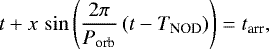
where T0 represents the reference epoch for the timing solution, Δν0 = (ν0 − ν‾) is the correction at the reference epoch of the spin frequency used to epoch-fold the data, ν˙ is the spin frequency derivative, and Rorb is the Roemer delay generated by the differential corrections to the ephemeris applied to correct the photon time of arrivals (e.g. Deeter et al. 1981). This process was iterated for each new set of orbital parameters obtained from the analysis until no significant differential corrections were found for the parameters of the model. Best-fit parameters with and without a spin frequency derivative are shown in Table 1. The measured derivative is several orders of magnitudes larger than typically observed in AMXPs, and we thus ascribe it to the NuSTAR internal clock drift, following a number of previous findings in the literature (Madsen et al. 2015; Sanna et al. 2017a,b,c). Figure 2 shows the pulse phase delays with the best-fitting model (top panel), and the corresponding residuals with respect to the model including a linear (middle panel) and a quadratic component (bottom panel) to fit the time evolution of pulse phase delays, respectively.
(3)
where T0 represents the reference epoch for the timing solution, Δν0 = (ν0 − ν‾) is the correction at the reference epoch of the spin frequency used to epoch-fold the data, ν˙ is the spin frequency derivative, and Rorb is the Roemer delay generated by the differential corrections to the ephemeris applied to correct the photon time of arrivals (e.g. Deeter et al. 1981). This process was iterated for each new set of orbital parameters obtained from the analysis until no significant differential corrections were found for the parameters of the model. Best-fit parameters with and without a spin frequency derivative are shown in Table 1. The measured derivative is several orders of magnitudes larger than typically observed in AMXPs, and we thus ascribe it to the NuSTAR internal clock drift, following a number of previous findings in the literature (Madsen et al. 2015; Sanna et al. 2017a,b,c). Figure 2 shows the pulse phase delays with the best-fitting model (top panel), and the corresponding residuals with respect to the model including a linear (middle panel) and a quadratic component (bottom panel) to fit the time evolution of pulse phase delays, respectively.
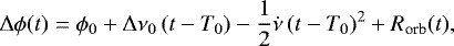
In Fig. 3 we show the best pulse profile obtained by epoch-folding the NuSTAR data with the parameters reported in Table 1 and sampling the signal in 100 phase bins. The peculiar pulse shape is well fitted with a combination of four sinusoids, where the fundamental, second, third, and fourth harmonics have fractional amplitudes of ~14%, ~4%, ~3.8%, and ~0.9%, respectively. The presence of harmonics of the fundamental frequency is consistent with the results shown in the PDS in Fig. 1.
Using the orbital binary parameters estimated from the NuSTAR timing analysis, we corrected the photon arrival times collected with Swift/XRT. We applied epoch-folding search techniques around the spin frequency reported in Table 1 with frequency steps of 10−5 Hz for a total of 101 steps. We significantly detected X-ray pulsations at the frequency ν = 105.1757(2) Hz, consistent within errors with the value obtained from the NuSTAR data.
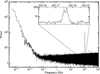 |
Fig. 1 Leahy-normalised (Leahy et al. 1983) PDS, produced by averaging 4096 s long segments of NuSTAR data. The fundamental frequency (~105 Hz) as well as the second and third harmonic are clearly visible in the power spectrum. The inset shows a zoom of the double-peaked profile of the fundamental frequency. |
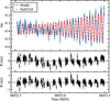 |
Fig. 2 Top panel: pulse phase delays as a function of time computed by epoch-folding ~250 s long intervals of NuSTAR data, together with the best-fit model (red dotted line, see text). Middle panel: residuals in ms with respect to the best-fit orbital solution including a linear model for the pulse phase delays. Bottom panel: residuals in ms with respect to the best-fit orbital solution including a quadratic model for the pulse phase delays. |
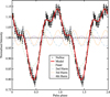 |
Fig. 3 Pulse profile (black points) obtained from the epoch-folded NuSTAR data. The best-fit model obtained by combining four sinusoids with harmonically related periods is also shown (red line). Two cycles of the pulse profile are shown for clarity. |
3.2 Spectral analysis
We performed a spectral analysis with Xspec 12.9.1n (Arnaud 1996) and fit near-simultaneous spectra in the 0.5–10 keV range for Swift/XRT, 3–78 keV for NuSTAR, and 20–100 keV for IBIS/ISGRI (Fig. 4). We assumed Wilms et al. (2000) elemental abundances and Verner et al. (1996) photo-electric cross-sections to model the interstellar medium. We allowed for a normalisation coefficient between instruments to account for cross-instrument calibration offsets and the possibility of source variation.
The spectra are well described ( /d.o.f. = 1.02/652) by an absorbed disk blackbody plus thermally comptonised continuum with seed photons from the blackbody radiation (const×tbabs×[diskbb+nthcomp] in Xspec). The measured absorption column density of (8.2 ± 1.0) × 1021 cm–2 is consistentwith that expected in the direction of the source (~9.5 × 1021 cm–2 ) using the cluster AV (Harris 1996, 2010 revision) and the appropriate conversion from AV to NH assuming Wilms abundances (Bahramian et al. 2015; Foight et al. 2016). We obtained from the fit an inner disk temperature of 1.42 ± 0.07 keV, a power-law photon index of
  , a blackbody seed photon temperature of 2.6 ± 0.1 keV, and a (poorly constrained) electron temperature of ~30 keV. We found no evidence for spectral lines (e.g. iron K-α) or reflection humps.
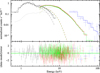 |
Fig. 4 Broad-band spectrum of IGR J16597–3704 (Swift in black, NuSTAR FPMA (FPMB) in red (green), and IBIS/ISGRI in blue). The dashed and dotted lines represent the disk-blackbody and comptonisation components of our model, respectively. |
4 Discussion
With the discovery of pulsations at ~105 Hz from IGR J16597–3704 and the measurement of its orbital period at almost 46 min, we identify the source as the 20th known AMXP and a new member of the ultracompact low-mass X-ray binaries. The X-ray spectrum of IGR J16597–3704 is typical for an AMXP in outburst (e.g. Falanga et al. 2013), and the non-detection of radio pulsations at the time of the Parkes observation is compatible with the fact that the X-ray outburst was still on-going. Assuming a typical pulsar spectral index of 1.6,the source previously detected at the VLA at 10 GHz (Tetarenko et al. 2017) would have a 1.4 GHz flux of 0.4 mJy. This would imply that the emission detected at the VLA is not pulsed and is most likely related to a radio jet.
The system mass function f(m2, m1, i) ~ 1.2 × 10⁻⁷ M⊙ and the lackof eclipses or dips in the X-ray light curve of the source allowus to constrain the mass of the donor star (m2 ). Considering an upper limit on the system inclination angle of i ≲ 75° (suggested by the absence of eclipses or dips in its light curve) and assuming a 1.4 M⊙ (2 M⊙) NS, we obtain m2 ≳ 0.0065 M⊙ (m2 ≳ 0.008 M⊙). This is consistent with the expected companion mass of ~0.01 M⊙ for an ultracompact NS binary in a 46-min orbital period (e.g. van Haaften et al. 2012). While the orbital properties of the system allow for a lower inclination angle and a higher mass, the requirement that the star must also fill its Roche lobe disfavours the higher mass solutions.
Given the measured unabsorbed flux of ~6.5 × 10⁻¹⁰ erg s–1 cm2 (0.5–100 keV), we estimate a source luminosity L = 6.5 × 1036 erg s–1 . Under the assumption that the torques on the accreting X-ray pulsar are in equilibrium, we make a rough estimate of the dipolar magnetic field of the NS:
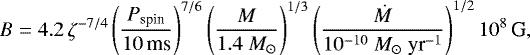 (4)
where ζ is a model-dependent dimensionless factor ranging between 0.1 and 1 that describes the relation between the magnetospheric radius and the Alfvén radius (see e.g. Ghosh & Lamb 1979; Wang 1996; Bozzo et al. 2009), Pspin represents the pulsar spin period in ms, M is the NS mass, and Ṁ is the rate of mass accreted onto the NS surface. Assuming an NS with R = 10 km and mass M = 1.4 M⊙, we obtain
(4)
where ζ is a model-dependent dimensionless factor ranging between 0.1 and 1 that describes the relation between the magnetospheric radius and the Alfvén radius (see e.g. Ghosh & Lamb 1979; Wang 1996; Bozzo et al. 2009), Pspin represents the pulsar spin period in ms, M is the NS mass, and Ṁ is the rate of mass accreted onto the NS surface. Assuming an NS with R = 10 km and mass M = 1.4 M⊙, we obtain  yr−1 and a dipolar magnetic field of 9.2 × 10⁸ < B < 5.2 × 10¹⁰ G. This is significantly larger than the average magnetic field of known AMXPs (see e.g. Mukherjee et al. 2015; Degenaar et al. 2017). Combined with the higher-than-average spin period of the source, this magnetic field suggests that IGR J16597–3704 is being observed in a relatively early stage of its recycling process. The mass required to spin up an old slowly rotating NS to ~105 Hz (of the order of 10−3 M⊙; e.g. Burderi et al. 1999) does not efficiently suppress the dipolar magnetic field, which limits the NS spin period. The large magnetic field combined with the moderately long spin period could be also responsible for the structured pulse profile, as well as for the lack of emission lines and reflection components in the energy spectrum.
Acknowledgments
We thank the NuSTAR, Swift, and Parkes teams for the rapid scheduling of the ToO observation of IGR J16597–3704. D. A. acknowledges support from the Royal Society. N. D. is supported by a Vidi grant awarded by The Netherlands organization for scientific research (NWO). We acknowledge financial contribution from the agreement ASI-INAF I/037/12/0, and the International Space Science Institute (ISSI) Bern, which funded and hosted the international team “The disk-magnetosphere interaction around transitional millisecond pulsars”. The Parkes radio telescope is part of the Australia Telescope National Facility which is funded by the Australian Government for operation as a National Facility managed by CSIRO. C. O. H. and G. R. S. are supported by NSERC Discovery Grants. A. P. acknowledges funding from the EUs Horizon 2020 Framework Programme for Research and Innovation under the Marie Skłodowska-Curie Individual Fellowship grant agreement 660657-TMSP-H2020-MSCA-IF-2014.
References
- Alpar, M. A., Cheng, A. F., Ruderman, M. A., & Shaham, J. 1982, Nature, 300, 728 [NASA ADS] [CrossRef] [Google Scholar]
- Altamirano, D., Patruno, A., Heinke, C. O., et al. 2010, ApJ, 712, L58 [NASA ADS] [CrossRef] [Google Scholar]
- Arnaud, K. A. 1996, in Astronomical Data Analysis Software and Systems V, eds. G. H. Jacoby, & J. Barnes, ASP Conf. Ser., 101, 17 [NASA ADS] [Google Scholar]
- Bahramian, A., Altamirano, D., Heinke, C., et al. 2015, ATel, 7242, 1 [NASA ADS] [Google Scholar]
- Bozzo, E., Stella, L., Vietri, M., & Ghosh, P. 2009, A&A, 493, 809 [NASA ADS] [CrossRef] [EDP Sciences] [Google Scholar]
- Bozzo, E., Grinberg, V., Wilms, J., et al. 2017a, ATel, 10880 [Google Scholar]
- Bozzo, E., Grinberg, V., Wilms, J., et al. 2017b, ATel, 10881 [Google Scholar]
- Burderi, L., & Di Salvo, T. 2013, Mem. Soc. Astron. It., 84, 117 [NASA ADS] [Google Scholar]
- Burderi, L., Possenti, A., Colpi, M., Di Salvo, T., & D’Amico, N. 1999, ApJ, 519, 285 [NASA ADS] [CrossRef] [Google Scholar]
- Cordes, J. M., & Lazio, T. J. W. 2002, ArXiv e-prints [arXiv:astro-ph/0207156] [Google Scholar]
- Courvoisier, T., Walter, R., Beckmann, V., et al. 2003, A&A, 411, L53 [NASA ADS] [CrossRef] [EDP Sciences] [Google Scholar]
- Deeter, J. E., Boynton, P. E., & Pravdo, S. H. 1981, ApJ, 247, 1003 [NASA ADS] [CrossRef] [Google Scholar]
- Degenaar, N., Pinto, C., Miller, J. M., et al. 2017, MNRAS, 464, 398 [NASA ADS] [CrossRef] [Google Scholar]
- Falanga, M., Kuiper, L., Poutanen, J., et al. 2013, ArXiv e-prints [arXiv:1302.2843] [Google Scholar]
- Foight, D. R., Güver, T., Özel, F., & Slane, P. O. 2016, ApJ, 826, 66 [NASA ADS] [CrossRef] [Google Scholar]
- Galloway, D. K., Chakrabarty, D., Morgan, E. H., & Remillard, R. A. 2002, ApJ, 576, L137 [NASA ADS] [CrossRef] [Google Scholar]
- Gehrels, N., Chincarini, G., Giommi, P., et al. 2004, ApJ, 611, 1005 [NASA ADS] [CrossRef] [Google Scholar]
- Ghosh, P., & Lamb, F. K. 1979, ApJ, 232, 259 [NASA ADS] [CrossRef] [Google Scholar]
- Harris, W. E. 1996, AJ, 112, 1487 [NASA ADS] [CrossRef] [Google Scholar]
- Harrison, F. A., Craig, W. W., Christensen, F. E., et al. 2013, ApJ, 770, 103 [NASA ADS] [CrossRef] [Google Scholar]
- Kirsch, M. G. F., Mukerjee, K., Breitfellner, M. G., et al. 2004, A&A, 423, L9 [NASA ADS] [CrossRef] [EDP Sciences] [Google Scholar]
- Krimm, H. A., Markwardt, C. B., Deloye, C. J., et al. 2007, ApJ, 668, L147 [NASA ADS] [CrossRef] [Google Scholar]
- Leahy, D. A., Darbro, W., Elsner, R. F., et al. 1983, ApJ, 266, 160 [NASA ADS] [CrossRef] [Google Scholar]
- Lebrun, F., Leray, J. P., Lavocat, P., et al. 2003, A&A, 411, L141 [NASA ADS] [CrossRef] [EDP Sciences] [Google Scholar]
- Lund, N., Budtz-Jørgensen, C., Westergaard, N. J., et al. 2003, A&A, 411, L231 [NASA ADS] [CrossRef] [EDP Sciences] [Google Scholar]
- Madsen, K. K., Harrison, F. A., Markwardt, C. B., et al. 2015, ApJS, 220, 8 [NASA ADS] [CrossRef] [Google Scholar]
- Markwardt, C. B., Swank, J. H., Strohmayer, T. E., in ’t Zand, J. J. M., & Marshall, F. E. 2002, ApJ, 575, L21 [Google Scholar]
- Mukherjee, D., Bult, P., van der Klis, M., & Bhattacharya, D. 2015, MNRAS, 452, 3994 [NASA ADS] [CrossRef] [Google Scholar]
- Papitto, A., Ferrigno, C., Bozzo, E., et al. 2013, Nature, 501, 517 [NASA ADS] [CrossRef] [PubMed] [Google Scholar]
- Patruno, A., & Watts, A. L. 2012, ArXiv e-prints [arXiv:1206.2727] [Google Scholar]
- Patruno, A., Haskell, B., & Andersson, N. 2017, ApJ, 805, 106 [NASA ADS] [CrossRef] [Google Scholar]
- Sanna, A., Di Salvo, T., Burderi, L., et al. 2017a, MNRAS, 471, 463 [NASA ADS] [CrossRef] [Google Scholar]
- Sanna, A., Papitto, A., Burderi, L., et al. 2017b, A&A, 598, A34 [NASA ADS] [CrossRef] [EDP Sciences] [Google Scholar]
- Sanna, A., Pintore, F., Bozzo, E., et al. 2017c, MNRAS, 466, 2910 [NASA ADS] [CrossRef] [Google Scholar]
- Schnitzeler, D. H. F. M. 2012, MNRAS, 427, 664 [NASA ADS] [CrossRef] [Google Scholar]
- Taylor, J. H., & Cordes, J. M. 1993, ApJ, 411, 674 [NASA ADS] [CrossRef] [Google Scholar]
- Tetarenko, A. J., Bahramian, A., Sivakoff, G. R., et al. 2017, ATel, 10894 [Google Scholar]
- Ubertini, P., Lebrun, F., Di Cocco, G., et al. 2003, A&A, 411, L131 [NASA ADS] [CrossRef] [EDP Sciences] [Google Scholar]
- Valenti, E., Ferraro, F. R., & Origlia, L. 2007, AJ, 133, 1287 [NASA ADS] [CrossRef] [Google Scholar]
- van Haaften, L. M., Nelemans, G., Voss, R., Wood, M. A., & Kuijpers, J. 2012, A&A, 537, A104 [NASA ADS] [CrossRef] [EDP Sciences] [Google Scholar]
- Verner, D. A., Ferland, G. J., Korista, K. T., & Yakovlev, D. G. 1996, ApJ, 465, 487 [NASA ADS] [CrossRef] [Google Scholar]
- Wang, Y.-M. 1996, ApJ, 465, L111 [NASA ADS] [CrossRef] [Google Scholar]
- Welsh, W. F., Robinson, E. L., & Young, P. 2000, AJ, 120, 943 [NASA ADS] [CrossRef] [Google Scholar]
- Wilms, J., Allen, A., & McCray, R. 2000, ApJ, 542, 914 [NASA ADS] [CrossRef] [Google Scholar]
- Yao, J. M., Manchester, R. N., & Wang, N. 2017, ApJ, 835, 29 [NASA ADS] [CrossRef] [Google Scholar]
All Tables
Orbital parameters and spin frequency of IGR J16597–3704 estimated from the NuSTAR data without a frequency derivative (left) and including a frequency derivative (right).
All Figures
|
Fig. 1 Leahy-normalised (Leahy et al. 1983) PDS, produced by averaging 4096 s long segments of NuSTAR data. The fundamental frequency (~105 Hz) as well as the second and third harmonic are clearly visible in the power spectrum. The inset shows a zoom of the double-peaked profile of the fundamental frequency. |
| In the text | |
|
Fig. 2 Top panel: pulse phase delays as a function of time computed by epoch-folding ~250 s long intervals of NuSTAR data, together with the best-fit model (red dotted line, see text). Middle panel: residuals in ms with respect to the best-fit orbital solution including a linear model for the pulse phase delays. Bottom panel: residuals in ms with respect to the best-fit orbital solution including a quadratic model for the pulse phase delays. |
| In the text | |
|
Fig. 3 Pulse profile (black points) obtained from the epoch-folded NuSTAR data. The best-fit model obtained by combining four sinusoids with harmonically related periods is also shown (red line). Two cycles of the pulse profile are shown for clarity. |
| In the text | |
|
Fig. 4 Broad-band spectrum of IGR J16597–3704 (Swift in black, NuSTAR FPMA (FPMB) in red (green), and IBIS/ISGRI in blue). The dashed and dotted lines represent the disk-blackbody and comptonisation components of our model, respectively. |
| In the text | |
Current usage metrics show cumulative count of Article Views (full-text article views including HTML views, PDF and ePub downloads, according to the available data) and Abstracts Views on Vision4Press platform.
Data correspond to usage on the plateform after 2015. The current usage metrics is available 48-96 hours after online publication and is updated daily on week days.
Initial download of the metrics may take a while.