| Issue |
A&A
Volume 610, February 2018
|
|
|---|---|---|
| Article Number | A87 | |
| Number of page(s) | 5 | |
| Section | Cosmology (including clusters of galaxies) | |
| DOI | https://doi.org/10.1051/0004-6361/201732181 | |
| Published online | 09 March 2018 | |
Evidence of a truncated spectrum in the angular correlation function of the cosmic microwave background
1
Department of Physics, The Applied Math Program, and Department of Astronomy, The University of Arizona,
AZ
85721, USA
e-mail: This email address is being protected from spambots. You need JavaScript enabled to view it.
2
Instituto de Astrofísica de Canarias,
38205
La Laguna,
Tenerife, Spain
3
Departamento de Astrofísica, Universidad de La Laguna,
38206
La Laguna,
Tenerife, Spain
Received:
26
October
2017
Accepted:
21
December
2017
Abstract
Aim. The lack of large-angle correlations in the fluctuations of the cosmic microwave background (CMB) conflicts with predictions of slow-roll inflation. But while probabilities (≲0.24%) for the missing correlations disfavour the conventional picture at ≳3σ, factors not associated with the model itself may be contributing to the tension. Here we aim to show that the absence of large-angle correlations is best explained with the introduction of a non-zero minimum wave number kmin for the fluctuation power spectrum P(k).
Methods. We assumed that quantum fluctuations were generated in the early Universe with a well-defined power spectrum P(k), although with a cut-off kmin ≠ 0. We then re-calculated the angular correlation function of the CMB and compared it with Planck observations.
Results. The Planck 2013 data rule out a zero kmin at a confidence level exceeding 8σ. Whereas purely slow-roll inflation would have stretched all fluctuations beyond the horizon, producing a P(k) with kmin = 0 – and therefore strong correlations at all angles – a kmin ≠ 0 would signal the presence of a maximum wavelength at the time (tdec) of decoupling. This argues against the basic inflationary paradigm, and perhaps even suggests non-inflationary alternatives, for the origin and growth of perturbations in the early Universe. In at least one competing cosmology, the Rh = ct universe, the inferred kmin corresponds to the gravitational radius at tdec.
Key words: cosmic background radiation / cosmology: observations / cosmology: theory / early Universe / inflation / large-scale structure of Universe
© ESO, 2018
1 Introduction
The Wilkinson Microwave Anisotropy Probe (WMAP; Bennett et al. 2003; Spergel et al. 2003) and Planck (Planck Collaboration XII 2014) have resoundingly confirmed the existence of several anomalies seen on very large scales by the Cosmic Background Explorer (COBE; Wright et al. 1996; Hinshaw et al. 1996). The most prominent among these is the lack of any significant correlation measured at angles ≳60∘. Its possible impact on the basic inflationary paradigm (Guth 1981; Linde 1982) has spurred a prolonged debate concerning whether it is due to a real physical phenomenon or unrecognized observational systematic effects.
The absence of large-angle correlations may simply be due to cosmic variance (Bennett et al. 2013; Copi et al. 2015), although probabilities for the missing correlations are typically ≲0.24%, disfavouring the basic inflationary picture at better than 3σ (see also Kim & Naselsky 2011; Melia 2014; Gruppuso et al. 2016). This anomaly may also be due to subtleties in the foreground subtraction or unrecognized instrumental systematics (Bennett et al. 2013), but this is far from settled.
The absence of large-angle correlations in the high-fidelity cosmic microwave background (CMB) maps poses one of the most serious challenges to the basic inflationary paradigm and, with it, to the internal self-consistency of the standard model. Since no theoretical corrections can improve the fit (Planck Collaboration XII 2014), the largest angular scales are probing different physics than the anisotropies seen at angles smaller than ~2∘ which, in contrast, are highly consistent with the predictions of the standard model.
In parallel with this dichotomy between the small- and large-angle correlations, WMAP and Planck have also revealed an unexpectedly weak power in the low-ℓ multipoles (see Eq. (6) below) compared with the corresponding power at higher ℓ’s (see e.g. Bennett et al. 2011). This anomaly may or may not be related to the absence of angular correlation at angles ≥60∘ (Copi et al. 2007, 2015). Arguments have been made on both sides, although, if unrelated, the existence of two such anomalies significantly exacerbates the tension with the predictions of standard inflationary cosmology (see also Efstathiou 2004). The power deficit at large angular scales manifests itself in several ways, however, not just via these two particular facets, so its impact on the interpretation of the CMB fluctuations is extensive. A thorough consideration of the broader issues associated with the low angular power may be found in several recent publications by the Planck Collaboration XXIII (2014) and Planck Collaboration XVI (2016). In this paper, our focus is specifically on the interpretation of the angular correlation function, which may now be studied at an unprecedented level of precision.
Previous attempts at modifying the basic inflationary paradigm to address this issue have relied on the inflaton field evolving through an early fast-rolling stage, producing a characteristic scale when the wave number associated with the transition from fast to slow roll exited the horizon (Contaldi et al. 2003; Destri et al. 2010; Gruppuso et al. 2016). However, given the relative imprecision of the data available then (compared to the exquisite measurements provided most recently by Planck), the existence of such a scale could be established at no more than ~ 2σ.
In one such attempt to determine whether the power spectrum is truncated, Niarchou et al. (2004) adopted a functional form (first introduced by Contaldi et al. 2003)
![Mathematical equation: \begin{equation} P(k) = P_0(k)[1-\mathrm{e}^{-(k/k_\mathrm{c})^\alpha}],\label{eq1} \end{equation}](/articles/aa/full_html/2018/02/aa32181-17/aa32181-17-eq1.png) (1)where
(1)where
 (2)
(2)
is the usual primordial power-law spectrum, kc is a characteristic wave number, and α = 1.8, and carried out a Bayesian model comparison based on the CMB power spectrum itself (rather than the angular correlation function) to demonstrate that the WMAP data available at that time preferred an attenuated P(k) with kc ≈ (5–6) × 10−4 Mpc−1 . If the last scattering surface occurred at zcmb ~ 1080 (according to the standard model), for which the expansion factor in a flat Universe was a(zcmb) = 1∕(1 + zcmb) ≈ 9.25 × 10⁻⁴, this characteristic wave number would have corresponded to a physical fluctuation size λmax ~ 10 Mpc. But for reasons we describe shortly, this use of the entire spectrum does not emphasize the large-angle anomalies, and Niarchou et al. (2004) concluded that a cut-off model such as Eq. (1) is preferred over one without a kc at only the ~1.4σ level.
In this paper, we address the observed lack of angular correlation at large angles with a clear, unobstructed focus on the possible existence of a cut-off in the fluctuation spectrum as seen primarily at angles ≫1∘, bolstered by the unprecedented accuracy of the Planck 2013 measurements. This distinctly different approach to the resolution of this anomaly avoids an unnecessary reliance on inflation, which may or may not have actually happened. A clear emergence of a non-zero kmin in the Planck data would motivate the search for new physics in both inflationary and non-inflationary scenarios. We note that the horizon problem plaguing Λ cold dark matter (CDM) manifests itself only in models with an early period of deceleration, so inflation is not required in all Friedmann–Robertson–Walker cosmologies. For example, it is not present in models, such as the Rh = ct universe (Melia 2007, 2016, 2017; Melia & Shevchuk 2012), in which opposite sides of the sky reached thermal equilibrium following the Big Bang (Melia 2013). In this paper, we seek to uncover compelling evidence in favour of such new physics beyond conventional, slow-roll inflation.
2 Theoretical background
To implement the introduction of a kmin, we assume that quantum fluctuations were generated in the early Universe with a well-defined power spectrum P(k), and that these seeds subsequently grew linearly towards tdec. But unlike the conventional picture, we find that the most important property of P(k) that alleviates the anomaly is a non-zero value of the minimum wave number kmin, possibly due to an early transition from fast to slow roll, or generic to a variety of non-inflationary scenarios. The Rh = ct universe, which has been studied extensively in recent years, meets these criteria, therefore we know of at least one alternative cosmology with the necessary characteristics (Melia 2016).
In the current ΛCDM, the fluctuations would have grown to all observable scales as a result of the rapid expansion during inflation, hence kmin = 0. In contrast, a non-inflationary expansion would have had kmin ≠ 0 if the fluctuation growth was restricted to a finite range of wavelengths. Again resorting to Rh = ct as an example, kmin could have corresponded to 2π times the Hubble radius Rh(tdec) at tdec. A similar correspondence would have applied to the formation of structure from topological defects (Brandenberger 1994). The results of our analysis should be independent of any specific model and relevant to any modified mechanism of inflation or to any non-inflationary cosmology that possesses a non-zero minimum wave number in its power spectrum P(k).
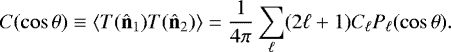
We follow convention and assume that a Gaussian random field in the plane of the sky describes the microwave temperature T(n̂) in every direction n̂, and write itas an expansion in spherical harmonics Ylm(n̂). The corresponding random coefficients alm have zero mean, hence the angular correlation function linking directions n̂1 and n̂2 depends only on θ ≡ n̂1⋅n̂1, which we expand in terms of Legendre polynomials as follows:
 (3)
(3)
The coefficients are statistically independent, therefore
 (4)
(4)
and statistical isotropy guarantees that the constant of proportionality depends only on ℓ,
 (5)
(5)
The expansion coefficient in Eq. (3),
 (6)
(6)
is known as the angular power of multipole ℓ.
In the ideal case of full-sky coverage, C(cos θ) provides a complementary means of analysing CMB observations instead of the angular power spectrum Cℓ . In principle, C(cos θ) contains the same information as the angular power spectrum, but it provides an easier understanding of the anisotropic structures and may serve as a complementary means of spherical-harmonic analysis, which is the most commonly used method. Some authors (Smoot et al. 1992; Hinshaw et al. 1996; Kashlinsky et al. 2001; Copi et al. 2015; López-Corredoira & Gabrielli 2013) have already attempted a direct determination of the anisotropies correlation function directly in angular space.
Several physical influences contribute to Cℓ , some preferentially at large angles (i.e. θ ≫ 1–2∘), others, suchas baryon acoustic oscillations (BAO), predominantly on smaller scales (Meiksin et al. 1999; Seo & Eisenstein 2005; Jeong & Komatsu 2006; Crocce & Scoccimarro 2006; Efstathiou et al. 2007; Padmanabhan & White 2009). The 2013 release of the Planck temperature power spectrum (Planck Collaboration XII 2014) up to ℓ = 30 is shown in Fig. 1, along with two theoretical fits that we discuss shortly. In this figure, Dℓ ≡ℓ(ℓ + 1)Cℓ∕2π. The well-known dichotomy between effects at large and small angles allows us to greatly simplify the calculation of Cℓ for the purpose of this paper. At large angles, corresponding to ℓ ≲ 30, the dominant physical process producing the anisotropies is the Sachs–Wolfe (SW) effect (Sachs & Wolfe 1967), representing metric perturbations associated with scalar fluctuations in the matter field. This effect relates the anisotropies observed in the temperature today to inhomogeneities of the metric fluctuation amplitude on the surface of last scattering. For the power-law spectrum of perturbations in Eq. (2), and assuming only SW, the angular power (Eq. (6)) reduces to the integral expression (Bond & Efstathiou 1984; Hu & Sugiyama 1995)
 (7)
(7)
where jℓ is the spherical Bessel function of order ℓ, and cΔτdec is the comoving radius of the last scattering surface written in terms of the conformal time difference between t0 and tdec. The normalization constant N is typically determined by optimizing the fit to the data in Fig. 1, although in this paper we also show the impact of optimizing N for C(cos θ). We stress that the key difference between the conventional approach and the novel idea we are introducing here is the appearance of a non-zero lower limit, kmin, to the integral in Eq. (7). As we see shortly, it is this kmin that accounts for the absence of CMB angular correlations at angles ≳60∘, representing a characteristic spatial scale apparently equal to 2π times the gravitational radius Rh(tdec) = c∕H(tdec) at decoupling.
From the WMAP and Planck observations, we infer that the power spectrum in Eq. (2) is very nearly scale free with n ≈1 (Planck Collaboration XII 2014). Therefore, selecting this value in Eq. (7), and defining the variable
 (8)
(8)
we may recast the expression for Cℓ in the form
 (9)
(9)
The constant umin is 2π times the number of proper maximum wavelengths λmax (corresponding to kmin) in the proper distance to the last scattering surface at tdec . Its value allows us to determine the angular size θmax of the largest fluctuation on this surface, using the expression
 (10)
(10)
where a(t) is the expansion factor. Therefore using the standard definition of the angular-diameter distance, this simply reduces to the form θmax = 2π∕umin.
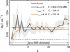 |
Fig. 1 Power spectrum (black) estimated with the NILC method (Planck Collaboration XII 2014), with 1σ Fisher errors (grey shaded). The Planck Λ CDM best fit model, including solely the Sachs–Wolfe (SW) effect, is shown in blue. The red curve for umin ≠ 0, andthe dashed curve for umin = 0, also based solely on SW, are optimized based on the best fit to C(cos θ) shown in Fig. 2. The SW effect dominates at large angles ≫ 1– 2∘ , corresponding to ℓ ≲ 30, while local physical effects, e.g. BAO, dominate for ℓ ≳ 30. |
3 Discussion
The CMB angular correlation function C(θ) based on the Planck 2013 release (Planck Collaboration XII 2014) has been calculated by averaging all temperature pairs in the sky separated by angles θ inside bins of size 1∘. We used the component-separated CMB map resulting from the Needlet Internal Linear Combination (NILC) algorithm, downloaded from the Planck Legacy Archive (PLA1). This map was smoothed to an angular resolution of 1∘ and degraded to HEALPix2 (Górski et al. 2005) Nside = 64 (pixel size 0.92∘). In order to avoid foreground contamination from residual Galactic emission or point sources, we excluded from our analysis all pixels affected by the multiplication of the Commander, SEVEM, and SMICA masks, which keeps 67% of the sky; we did not take into account the NILC mask because it removes a significantly smaller fraction of the sky. The 1σ error bars were computed through a comparison of the angular correlation function calculated for 200 randomly rotated maps based on the original distribution.
The calculated angular power Cℓ for multipoles 2 ≤ ℓ ≤ 30 is shown for the conventional ΛCDM (blue curve) in Fig. 1, optimized to fit the Planck 2013 release. Also, for comparison, we show in this figure a fit for umin = 0 (dashed) optimized using C(cos θ) in Fig. 3 instead of the angular-power spectrum. In Fig. 1, the theoretical curves take into account only SW, ignoring the physical influences (such as BAO) that would dominate on small angular scales (i.e. at ℓ ≳ 30). It is well known that the latter depend, at most, only weakly on the cosmology, and are therefore degenerate among different models (Scott et al. 1995).
The fit for umin≠0 is optimized using C(cos θ) in Fig. 2. For the ΛCDM (blue) curve, we followed the conventional approach of first fitting the temperature spectrum to determine the normalization constant N in Eq. (9), which is then used together with Eq. (3) to produce the angular correlation function. It has been known since the early WMAP release (Spergel et al. 2003) that the ΛCDM curve is inconsistent with the measured C(cos θ), but when viewed here in comparison with the curve corresponding to umin≠0, its lack of adequate confirmation by the data is even more glaring. The red curve in Fig. 2 shows the best fit attainable with umin≠0. Based on the Planck 2013 data release, we find an optimized value umin = 4.34 ± 0.50, corresponding to a maximum fluctuation size θmax ≈ 83∘ in the plane of the sky. For comparison with the value of kc estimated earlier by Niarchou et al. (2004) using WMAP data, we determined for Λ CDM (in which zcmb = 1080) that this measurement of umin corresponds to a maximum fluctuation size λmax ~ 20 Mpc at decoupling, which is about twice the value corresponding to their characteristic wave number kc . Of course, with the benefit of using the more precise Planck data, and our focus on the large-angle anomalies rather than the entire CMB power spectrum, we also conclude that a cut-off in P(k) is favoured at a much higher level of significance than before, now in excess of ~ 8σ.
This σ = 0.5 error in the measurement of umin was obtained from a Monte Carlo analysis sampling the variation of C(cos θ) within the measurement errors. The C(cos θ) points are highly correlated, but our analysis circumvents this problem with the Monte Carlo procedure. First, we generated 100 mock CMBR catalogues [using standard cosmology with an angular function C0(cos θ)] and we measured the two-point correlation Ci(cos θ) in each case. From these, we obtained ΔCi(cos θ) ≡ Ci(cos θ) − Ci(cos θ) − C0(cos θ), and then calculated umin, i for C(cos θ) = CPlanck(cos θ) + ∆Ci(cos θ) for each realization i. Next, we examined the distribution of umin, i (which is roughly Gaussian) and determined its average value and the rms within which one finds 68 of the 100 values; this yields the quoted result umin = 4.34 ± 0.50. This is not equivalent to a simple χ2 fitting with the correlated error bars shown in Figs. 2 and 3. Such a simple χ2 procedure would instead have given  , i.e. a much smaller error for umin. This difference stems precisely from the fact that the C(cos θ) points are correlated. Therefore the 68% confidence limit for this value of umin suggests that a theoretical best fit to the measured angular correlation function with umin = 0 is rejected at 8.6 σ.
From Fig. 2 we see that there are several good reasons for preferring the umin = 4.34 fit over a model with umin = 0: (1) Planck has confirmed that C(cos θ) ≈ 0 at angles θ ≳ 60∘–70∘, in sharp contrast to the prediction of the conventional inflationary Λ CDM; (2) the model with umin = 4.34 correctly reproduces the minimum of C(cos θ) at ≈45∘–50∘; and (3) it actually fits the measured curve beyond ~ 50∘ quite well, which is fully consistent with the measurement errors.
Suppose we were to optimize C2 with umin = 0 based on the angular correlation data in Fig. 2, instead of the power spectrum in Fig. 1. This third case is shown as a dashed black curve in Fig. 3. Certainly, the fit to C(cos θ) has improved, although there is still significant tension with theory at θ≲ 20∘ and the best fit curve completely misses the minimum of C(cos θ) at θ~ 50∘. In addition,with this optimized value of C2 (i.e. 258.53 μK2), the theoretical angular power spectrum is now a very poor fit to the measured Dℓs shown in Fig. 1. By far, the best fit to the angular power spectrum and correlation function is realized when umin = 4.34 ± 0.50.
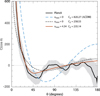 |
Fig. 3 Impact of umin on the angular correlation function with truncated inflation, or a non-inflationary cosmology. The conventional Λ CDM curve corresponds to umin = 0, i.e. an unconstrained inflationary power spectrum. The Planck measurement is shown as a black solid curve. |
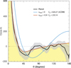 |
Fig. 2 Angular correlation function measured with Planck (dark solid curve) (Planck Collaboration XII 2014), and associated 1σ errors(grey), compared with the prediction of the conventional inflationary Λ CDM (blue). In this model one assumes that umin = 0 and then optimizes C2 using the power spectrum in Fig. 1. The red curve shows the prediction of truncated inflation, or a non-inflationary cosmology, with an optimized lower limit umin = 4.34 and C2 = 235.14. |
4 Conclusions
The S1∕2 statistic (Spergel et al. 2003) has traditionally been used to categorize the degree to which the measured angular correlation at large angles is deficient compared to theoretical predictions. This quantity is basically an integral of C(θ)2 over angles from (cos θ) = −1 to (cos θ) = 1/2. With Monte Carlo simulations, one can build a distribution of S1∕2 values, thereby assigning a probability that the observed angular correlation function could be drawn randomly as a result of cosmic variance from the predicted function. The p-values quoted earlier in this paper for conventional Λ CDM are estimated using this comparison.
Our analysis in this paper is superior to S1∕2 for several reasons. First, S1∕2 represents an integrated quantity, from θ ~ 60∘to 180∘, designed to find a deficiency in signal. Second, it completely ignores the comparison between theory and observation at angles ≲ 60∘, where the tension can be just a large as it is at θ ≳ 60∘. Both of these limitations with S1∕2 make it an inferior statistic to use in this work compared to our approach of actually fitting the C(θ) data by optimizing the value of umin. The fact that the conventional inflationary paradigm is disfavoured by these data in comparison to a model with kmin > 0 is supported by both approaches. But the optimization carried out in this paper goes significantly beyond this level by demonstrating that kmin = 0 is ruled out at a confidence level of ~8σ.
A k > kmin constraint on P(k) is inconsistent with purely slow-roll inflationary cosmology, which instead predicts that fluctuations would have exited and re-entered the horizon prior to decoupling, resulting in kmin = 0 and strong correlations at all angles. On the other hand, such a result is fully consistent with the predictions of the Rh = ct universe (Melia 2007, 2013; Melia & Shevchuk 2012), in which fluctuations might have emerged near the Planck scale, equal to the Hubble radius Rh at the Planck time. The kmin might therefore correspond to the horizon size at the surface of last scattering, since only fluctuations with λmax ~ 2πRh would have continued to grow towards tdec.
The fact that the measured CMB angular correlation function strongly favours modifying conventional inflation, or eliminating it all together, is an important validation of other recent results showing similar trends (Wei et al. 2016). Looking forward to the next generation of observations and simulations, the introduction of a non-zero kmin should be quite straightforward to implement. The introduction of a kmin will not affect many other kinds of observation. The optimized value we found here corresponds to a maximum fluctuation angle in the sky of about 83∘. As such, this will have no impact on the optimization of the power spectrum, since kmin affects only the far-left (i.e. ℓ ~ 1–10) portion of Dℓ in Fig. 1. By comparison, the first acoustic peak in the power spectrum is centred at ℓ ~ 200 corresponding to an angle of ~1∘. For similar reasons, such a large maximum fluctuation angle is unlikely to affect other measurements. At least for now, the focus with kmin should be on refining the measurement of the angular correlation function of the CMB.
From a simulational point of view, however, we have so far ignored the integrated Sachs Wolfe (ISW) effect, which arises owing to thepassage of light from the surface of last scattering to our location (Bond & Efstathiou 1984). The ISW is not negligible, although the early-time contribution is typically combined with SW at last scattering and is incorporated into Eq. (7). The late-time ISW is smaller, but nonetheless present, hence a complete accounting of the impact of kmin will eventually need to include its influence. We do not expect our results to change substantially.
Acknowledgments
We are very grateful to Ricardo Génova-Santos for help calculating the angular correlation function using the Planck 2013 data release. F.M. acknowledges partial support from the Chinese State Administration of Foreign Experts Affairs under grant GDJ20120491013. M.L.C. was supported by grant AYA2015-66506-P of the Spanish Ministry of Economy and Competitiveness.
References
- Bennett, C. L., Hill, R. S., Hinshaw, G., et al. 2003, ApJS, 148, 97 [NASA ADS] [CrossRef] [Google Scholar]
- Bennett, C. L., Hill, R. S., Hinshaw, G., et al. 2011, ApJS, 192, 17 [NASA ADS] [CrossRef] [Google Scholar]
- Bennett, C. L., Larson, D., Weiland, J. L. et al. 2013, ApJS, 208, 20 [Google Scholar]
- Bond, J. R., & Efstathiou, G. 1984, ApJ, 285, L45 [NASA ADS] [CrossRef] [Google Scholar]
- Brandenberger, R. H. 1994, IJMP-A, 9, 2117 [NASA ADS] [Google Scholar]
- Contaldi, C. R., Peloso, M., Kofman, L., & Linde, A. 2003, JCAP, 7, 002 [Google Scholar]
- Copi, C. J., Huterer, D., Schwarz, D. J., & Starkman, G. D. 2007, PRD, 75, 023507 [NASA ADS] [CrossRef] [Google Scholar]
- Copi, C. J., Huterer, D., Schwarz, D. J., & Starkman, G. D. 2015, MNRAS, 451, 2978 [NASA ADS] [CrossRef] [Google Scholar]
- Crocce, M., & Scoccimarro, R. 2006, PRD, 73, 063520 [Google Scholar]
- Destri, C., de Vega, H. J., & Sanchez, N. G. 2010, PRD, 81, 063520 [NASA ADS] [CrossRef] [Google Scholar]
- Efstathiou, D. J. 2004, MNRAS, 348, 885 [NASA ADS] [CrossRef] [Google Scholar]
- Eisenstein, D. J., Seo, H.-J., & White, M. 2007, ApJ, 664, 660 [NASA ADS] [CrossRef] [Google Scholar]
- Górski, K., Hivon, E., Banday, A. J., et al. 2005, ApJ, 622, 759 [NASA ADS] [CrossRef] [Google Scholar]
- Gruppuso, A., Kitazawa N., Mandolesi, N. P. N., Sagnotti, A. 2016, PDU, 11, 68 [NASA ADS] [Google Scholar]
- Guth, A. H. 1981, PRD, 23, 347 [Google Scholar]
- Hinshaw, G., Banday, A. J., Bennett, C. L., et al. 1996, ApJ, 464, L25 [NASA ADS] [CrossRef] [Google Scholar]
- Hu, W., & Sugiyama, N. 1995, ApJ, 444, 489 [NASA ADS] [CrossRef] [Google Scholar]
- Jeong, D., & Komatsu, E. 2006, ApJ, 651, 619 [NASA ADS] [CrossRef] [Google Scholar]
- Kashlinsky, A., Hernández-Monteagudo, A., & Atrio-Barandela, F. 2001, ApJ, 557, L1 [NASA ADS] [CrossRef] [Google Scholar]
- Kim, J., & Naselsky, P. 2011, ApJ, 739, 79 [NASA ADS] [CrossRef] [Google Scholar]
- Linde, A. 1982, PLB, 108, 389 [Google Scholar]
- López-Corredoira, M., & Gabrielli, A. 2013, Physica A, 392, 474 [NASA ADS] [CrossRef] [Google Scholar]
- Meiksin, A., White, M., & Peacock, J. A. 1999, MNRAS, 304, 851 [NASA ADS] [CrossRef] [Google Scholar]
- Melia, F. 2007, MNRAS, 382, 1917 [NASA ADS] [CrossRef] [Google Scholar]
- Melia, F. 2013, A&A, 553, A76 [NASA ADS] [CrossRef] [EDP Sciences] [Google Scholar]
- Melia, F. 2014, A&A, 561, A80 [NASA ADS] [CrossRef] [EDP Sciences] [Google Scholar]
- Melia, F. 2016, Front. Phys., 11, 118901 [Google Scholar]
- Melia, F. 2017, Front. Phys., 12, 129802 [CrossRef] [Google Scholar]
- Melia, F., & Shevchuk, A. 2012, MNRAS, 419, 2579 [NASA ADS] [CrossRef] [Google Scholar]
- Niarchou, A., Jaffe, A. H. & Pogosian, L. 2004, PRD, 69, 063515 [NASA ADS] [CrossRef] [Google Scholar]
- Padmanabhan, N., & White, M. 2009, PRD, 80, 063508 [NASA ADS] [CrossRef] [Google Scholar]
- Planck Collaboration XII 2014, A&A, 571, A12 [NASA ADS] [CrossRef] [EDP Sciences] [Google Scholar]
- Planck Collaboration XXIII 2014, A&A 571, A23 [NASA ADS] [CrossRef] [EDP Sciences] [MathSciNet] [PubMed] [Google Scholar]
- Planck Collaboration XVI 2016, A&A, 594, A16 [NASA ADS] [CrossRef] [EDP Sciences] [Google Scholar]
- Sachs, R. K., & Wolfe, A. M. 1967, ApJ, 147, 73 [NASA ADS] [CrossRef] [Google Scholar]
- Scott, D., Silk, J., & White, M. 1995, Science, 268, 829 [NASA ADS] [CrossRef] [PubMed] [Google Scholar]
- Seo, H.-J., & Eisenstein, D. J. 2005, ApJ, 633, 575 [NASA ADS] [CrossRef] [Google Scholar]
- Smoot, G. F., Bennett, C. L., Kogut, A., et al. 1992, ApJ, 396, L1 [NASA ADS] [CrossRef] [Google Scholar]
- Spergel, D. N., Verde, L., Peiris, H.V, et al. 2003, ApJS, 148, 175 [NASA ADS] [CrossRef] [Google Scholar]
- Wei, J.-J., Wu, X., & Melia, F. 2016, MNRAS, 463, 1144 [NASA ADS] [CrossRef] [Google Scholar]
- Wright, E. L., Bennett, C. L., Gorski, K., et al. 1996, ApJ, 464, L21 [NASA ADS] [CrossRef] [Google Scholar]
All Figures
|
Fig. 1 Power spectrum (black) estimated with the NILC method (Planck Collaboration XII 2014), with 1σ Fisher errors (grey shaded). The Planck Λ CDM best fit model, including solely the Sachs–Wolfe (SW) effect, is shown in blue. The red curve for umin ≠ 0, andthe dashed curve for umin = 0, also based solely on SW, are optimized based on the best fit to C(cos θ) shown in Fig. 2. The SW effect dominates at large angles ≫ 1– 2∘ , corresponding to ℓ ≲ 30, while local physical effects, e.g. BAO, dominate for ℓ ≳ 30. |
| In the text | |
|
Fig. 3 Impact of umin on the angular correlation function with truncated inflation, or a non-inflationary cosmology. The conventional Λ CDM curve corresponds to umin = 0, i.e. an unconstrained inflationary power spectrum. The Planck measurement is shown as a black solid curve. |
| In the text | |
|
Fig. 2 Angular correlation function measured with Planck (dark solid curve) (Planck Collaboration XII 2014), and associated 1σ errors(grey), compared with the prediction of the conventional inflationary Λ CDM (blue). In this model one assumes that umin = 0 and then optimizes C2 using the power spectrum in Fig. 1. The red curve shows the prediction of truncated inflation, or a non-inflationary cosmology, with an optimized lower limit umin = 4.34 and C2 = 235.14. |
| In the text | |
Current usage metrics show cumulative count of Article Views (full-text article views including HTML views, PDF and ePub downloads, according to the available data) and Abstracts Views on Vision4Press platform.
Data correspond to usage on the plateform after 2015. The current usage metrics is available 48-96 hours after online publication and is updated daily on week days.
Initial download of the metrics may take a while.