| Issue |
A&A
Volume 610, February 2018
|
|
|---|---|---|
| Article Number | A66 | |
| Number of page(s) | 10 | |
| Section | Galactic structure, stellar clusters and populations | |
| DOI | https://doi.org/10.1051/0004-6361/201732024 | |
| Published online | 02 March 2018 | |
NGC 6705 a young α-enhanced open cluster from OCCASO data★
1
Departament de Física Quàntica i Astrofísica, Universitat de Barcelona, ICC/IEEC,
08007
Barcelona, Spain
email: laiacf@fqa.ub.edu
2
INAF – Osservatorio Astronomico di Padova,
Padova, Italy
3
Leibniz-Institut für Astrophysik Potsdam (AIP),
Potsdam, Germany
4
Harvard-Smithsonian Center for Astrophysics,
Cambridge,
MA
02138, USA
5
INAF – Osservatorio Astrofisico di Arcetri,
50125
Firenze, Italy
6
ASI Science Data Center,
00133
Roma, Italy
7
Instituto de Astrofísica de Canarias,
La Laguna,
38205
Tenerife, Spain
8
Departamento de Astrofísica, Universidad de La Laguna,
38207
Tenerife, Spain
9
Space Telescope Science Institute,
Baltimore,
MD
21218, USA
Received:
2
October
2017
Accepted:
30
October
2017
Context. The stellar [α/Fe] abundance is sometimes used as a proxy for stellar age, following standard chemical evolution models for the Galaxy, as seen by different observational results. Aim. In this work, we aim to show that the open cluster NGC 6705/M 11 has a significant α-enhancement [α/Fe] > 0.1 dex, despite its young age (~300 Myr), challenging the current paradigm.
Methods. We used high resolution (R > 65 000) high signal-to-noise (~70) spectra of eight red clump stars, acquired within the OCCASO survey. We determined very accurate chemical abundances of several α elements, using an equivalent width methodology (Si, Ca and Ti), and spectral synthesis fits (Mg and O).
Results. We obtain [Si/Fe] = 0.13 ± 0.05, [Mg/Fe] = 0.14 ± 0.07, [O/Fe] = 0.17 ± 0.07, [Ca/Fe] = 0.06 ± 0.05, and [Ti/Fe] = 0.03 ± 0.03. Our results place these clusters within the group of young [α/Fe]-enhanced field stars recently found by several authors in the literature. The ages of our stars have an uncertainty of around 50 Myr, much more precise than for field stars. By integrating the cluster’s orbit in several non-axisymmetric Galactic potentials, we establish the M 11’s most likely birth radius as lying between 6.8–7.5 kpc from the Galactic centre, not far from its current position.
Conclusions. With the robust open cluster age scale, our results prove that a moderate [α/Fe]-enhancement is no guarantee for a star to be old, and that not all α-enhanced stars can be explained with an evolved blue straggler scenario. Based on our orbit calculations, we further argue against a Galactic bar origin of M 11.
Key words: Stars: abundances / open clusters and associations: individual: NGC 6705 (M 11)
Full Table 2 is only available at the CDS via anonymous ftp to cdsarc.u-strasbg.fr (130.79.128.5) or via http://cdsarc.u-strasbg.fr/viz-bin/qcat?J/A+A/610/A66
© ESO 2018
1 Introduction
The stellar [α/Fe] ratio has been widely used as an indirect age estimator because α-elements, for example O, Mg, Si, Ca, and Ti, are produced in short time scales by core collapse type II supernovae in comparison with iron, synthesized on longer timescales by type Ia supernovae (Matteucci 2001; Fulbright et al. 2007, among others). Therefore, as soon as type Ia supernovae, related to intermediate-mass binary systems with mass transfer, start to contribute to the iron enrichment, [α/Fe] inevitably decreases. In this scenario, an [α/Fe] enhancement means that the star was born in a gas mainly enriched by massive stars.
The correlation between [α/Fe] and age has been widely used in the literature to trace the different Galaxy components (e.g. Alves-Brito et al. 2010). From the analysis of HIPPARCOS stars in a local sphere with a radius of 25 pc, Fuhrmann (2011) assigned an age older than 10 Gyr to those stars with high [α/Fe] ratios and assumed that they belong to the chemical thick disc. However, recent analysis of larger samples outside the local volume has shown that [α/Fe] enhancement does not guarantee that a star is old. Chiappini et al. (2015) reported the existence of a young [α/Fe]-enhanced population from the analysis of a sample of 606 red giants observed by both CoRoT (Miglio et al. 2013) and APOGEE (Majewski et al. 2017). They showed that most of the stars follow the behaviour of α-element abundances predicted by standard evolution models. However, several young stars show unexpectedly high [α/Fe] abundances. Interestingly, most of these stars are located at small Galactocentric distances, around 6 kpc from the Galactic centre. Chiappini et al. (2015) also points out the fact that young α-enhanced stars are also present in other works available in the literature (e.g. Haywood et al. 2013; Bensby et al. 2014; Bergemann et al. 2014). Additionally, at least 14 stars with [α/Fe] > 0.13 and ages younger than 6 Gyr have been detected by Martig et al. (2015) in their analysis of the stars in common by both Kepler and APOGEE, known as APOKASC.
There are different possible scenarios to explain the origin of these young [α/Fe] enhanced stars. The first one is a possible ambiguity in determining ages from masses in asteroseismology, since higher masses are assigned to younger ages. As stated by Jofré et al. (2016) and Yong et al. (2016), α-rich stars may look young because they have accreted material from a binary companion or because they are a result of a binary merger (blue straggler). In this case, the mass would not reflect the real age of the progenitor star. In the case that these stars are genuinely young, they could have been formed from a recent gas accretion event. Another interpretation is that they could have been born in a region near the corotation of the bar where gas can be kept inert for a long time reflecting only type II supernovae ejecta. They could then have been kicked to their current location.
In this paper we focus on NGC 6705 (M 11), a young open cluster (OC) located in the inner disc (l, b) = (27.307∘, −2.776∘) at a Galactocentric distance of 6.8 kpc and very close to the plane at z = −90 pc (Dias et al. 2002). It has been extensively studied because it is among the most massive known OCs, containing several thousand solar masses(Santos et al. 2005). The age of NGC 6705 has been derived from isochrone fitting (e.g. Sung et al. 1999a; Santos et al. 2005; Beaver et al. 2013; Cantat-Gaudin et al. 2014b) and also from detached eclipsing binaries (Bavarsad et al. 2016). These studies all agree on an age of between ~0.2 and 0.3 Gyr. This OC has been targeted by two of the massive Galactic spectroscopic surveys, APOGEE and GES (Gilmore et al. 2012), with still controversial results about its chemical composition (Cantat-Gaudin et al. 2014b; Magrini et al. 2014, 2015, 2017; Tautvaišienė et al. 2015).
In the framework of the Open Cluster Chemical Abundances from Spanish Observatories survey (OCCASO; Casamiquela et al. 2016)we have obtained very high-resolution (R ~ 65 000–85 000), high signal-to-noise ratio (S∕N ≳ 70) spectra for eight stars in this cluster. We derived a mild α-enhancement which is still outside the expectations of standard chemical evolution models. In this paper, we present our chemical analysis of NGC 6705 and we discuss our results according to the chemical evolution models. The paper is organized as follows. In Sect. 2, the observational material used is presented. The spectroscopic analysis is detailed in Sect. 3, where we present stellar atmosphere parameters (Sect. 3.1) and chemical abundances (Sect. 3.2). An extensive comparison with literature is presented in Sect. 4. We compute the orbit of the cluster in the Galaxy under different assumptions in Sect. 5. A discussion of the results is given in Sect. 6, and the overall conclusions are presented in Sect. 7.
2 Observational material
OCCASO (see Casamiquela et al. 2016, hereafter referred to as Paper I, for a detailed description) is currently obtaining very high-resolution spectra (R ≿ 650 000) in the optical range (5000–8000 Å) for red clump stars in northern OCs. This survey systematically targets OCs that have at least six stars per cluster, and with a S∕N around 70. It is a natural complement to the GES-UVES observations of OCs from the north, and an optical counterpart for APOGEE.
The source NGC 6705 has been observed as part of the OCCASO survey. A total of eight stars have been observed with HERMES (Raskin et al. 2011) installed at Mercator Telescope (La Palma, Spain). Three of them were also observed with FIES (Telting et al. 2014) at Nordic Optical Telescope (La Palma, Spain) as part of a subsample designed for comparison between instruments. Details of the observed stars are listed in Table 1: coordinates, magnitude, instrument, S/N of the spectra, atmospheric parameters (see next section) and radial velocities. We also include the available membership information from previous studies: probabilities from proper motion and membership classification from radial velocity.
Radial velocities for the observed stars are presented in Paper I. All observed stars are compatible with being members from their radial velocities within 1σ. Since then, with new observational runs, we observed one more star (W1256) which has also a compatible radial velocity. The cluster mean radial velocity using the eight stars is 35 ± 1 km s−1.
In Fig. 1, we plot the position of the target stars in the colour-magnitude diagram from Sung et al. (1999b). We overplot a PARSEC isochrone (Bressan et al. 2012) with the age, metallicity, extinction and distance derived by Cantat-Gaudin et al. (2014b): age = 316 ± 50 Myr, Z = 0.019, E(B − V) = 0.40 ± 0.03, and V − MV = 11.45 ± 0.2 (d = 1950 ± 200 pc).
Details of the observed stars.
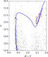 |
Fig. 1 Colour-magnitude diagram with the photometry from Sung et al. (1999b). Target stars are marked with red crosses.A PARSEC isochrone of age 316 Myr and Z = 0.019 shifted by V − MV = 11.45 (d = 1950 pc) and E(B − V) = 0.40 (Cantat-Gaudin et al. 2014b) is overplotted. |
3 Spectroscopic analysis using OCCASO data
3.1 Atmospheric parameters and iron abundance
Stellar atmospheric parameters and iron abundances for stars sampled by OCCASO were obtained by Casamiquela et al. (2017a, Paper II hereafter). Briefly, effective temperature Teff , surface gravity log g, microturbulence ξ, and iron abundances were derived using two independent methods: DAOSPEC (Cantat-Gaudin et al. 2014a; Stetson & Pancino 2008) + GALA (Mucciarelli et al. 2013) which uses the equivalent width (EW) methodology, and iSpec (Blanco-Cuaresma et al. 2014a) which uses the spectral synthesis fitting (SS) method. In both cases we adopted the MARCS atmosphere models from Gustafsson et al. (2008) computed assuming 1D-LTE, Grevesse et al. (2007) solar composition, and the standard α-enhancement at low metallicities. We used Version 5 of the master line list from GES (Heiter et al. 2015b) which covers the spectral range 4200 ≤ λ ≤ 9200 Å, and contains atomic information for 35 different chemical species. We refer the reader to Paper II for further details.
As explained in Paper II, the final stellar atmospheric parameters adopted for each star are the mean of the values obtained by these two methods. Obtained values in the plane Teff – log g are plotted in Fig. 2, and the same isochrone used in Fig. 1 is drawn as reference. The theoretical position of the red clump traced by this isochrone is well reproduced.
In Paper II, iron abundances were derived also with both methods separately but using the average Teff and log g described above. The average iron abundance of the cluster is [Fe/H]EW = 0.17 ± 0.04 and [Fe/H]SS = 0.04 ± 0.05, from the EW and the SS analysis, respectively. We refer the reader to Paper II for more details of the two calculations. In the current paper, we have used the value derived from EW since it is consistent with other determinations available in the literature.
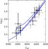 |
Fig. 2 Derived Teff and log g in Paper II. Grey points are the values of the stars observed with both FIES and HERMES. For these stars we also plot the mean values (in black). The same isochrone as in Fig. 1 is overplotted. |
3.2 Si, Ca, and Ti chemical abundances
The chemical abundances of Si, Ca, and Ti were obtained using the EW method. The EW analysis is performed in two steps. First, EWs are measured using DOOp (Cantat-Gaudin et al. 2014a), which is an automatic wrapper for DAOSPEC (Stetson & Pancino 2008). It finds absorption lines in a stellar spectrum, fits the continuum, measures EWs, identifies lines from a provided line list, and gives a radial velocity estimate. Obtained EWs are fed to GALA (Mucciarelli et al. 2013), which uses the set of Kurucz abundance calculation codes (Kurucz 2005; Sbordone et al. 2004) to derive chemical abundances. The lines that yield systematically discrepant abundances with respect to the mean abundance of the element are rejected. For this we used the spectra of all stars targeted by OCCASO (115 stars). This is a consistent procedure to discard blended features or lines with inaccurate atomic parameters, obtaining a robust sample of lines for chemical abundance determination from their EW.
The EWs obtained for the 11 analysed spectra are listed in Table 2. The uncertainties of the EW measurements are typically below 5%. For each spectrum we obtained the [X/Fe] ratio as the mean of the abundances derived from individual lines. These values are listed in Table 3. The errors in [X/Fe] for each star were estimated from the dispersion of the line abundances divided by the square root of the number of lines, quadratically summed to the error in [Fe/H].
Lines used to compute abundances of Si, Ca and Ti.
Final Si, Ca, Ti, Mg and O over Fe abundances of all the analysed stars.
3.3 Chemical abundances of O and Mg
To determine abundances of O and Mg we performed a SS analysis with Salvador (A. Mucciarelli, priv. comm.). Using this type of analysis we account for blends or hyperfine structure splitting, present in the lines of those elements. Salvador is a tool that fits individual lines from an observed spectrum with synthetic spectra. The spectra are synthesized using the set of Kurucz codes (Kurucz 2005; Sbordone et al. 2004) and the MARCS atmosphere models (Gustafsson et al. 2008) from the atmosphericparameters determined in Paper II in a window around a given spectral line. The region around the feature of interest is renormalized by the code using the ratio between the observed and the best-fit spectrum. Salvador allows the user to modify the normalization, the size of the window,and the abundances of the different chemical species involved with respect to the assumed by the model (used for blended lines).
Atomic information for the lines are indicated in Table 4. To determine the Mg abundances we used two lines at 5711.088, and 6318.717 Å, respectively. Their hyperfine structure splitting was taken into account in the line list. We used the mean of the two lines to derive the overall Mg abundance per spectrum. The mean of the errors determined for the two lines was used as error for [Mg/H], and we quadratically summed the error in [Fe/H] to determine σ[Mg/Fe]. The abundances for each line and spectra are listed in Table 5.
For oxygen we use the forbidden [O I] line at 6300.304 Å. It is well known that this feature is blended with a Ni I line (Allende Prieto et al. 2001), often neglected, but that has a high impact at solar and supersolar metallicities. The code has the option to fix an abundance variation of Ni to perform an accurate fit. So for each spectrum we set this to the Ni abundance derived with the EW methodology typically using around 25 lines. Since oxygen and carbon are bound together by the molecular equilibrium in stellar atmospheres, while determining the oxygen we have taken carbon abundances into account. We adopted the mean carbon abundance for the cluster to the value [C/H] = − 0.08 ± 0.06 derived by Tautvaišienė et al. (2015), to perform the fit with Salvador. The oxygen line could not be measured in W0686 because the large noise prevented us from properly determining the continuum. This was also the case for W1256, which has a sky line on top of it.
To compute the errors on the derived chemical abundances for each linewe took into account two sources of uncertainty: the errors due to the choice of the atmospheric parameters, and the errors due to the fit.
-
To account for the uncertainty due to the assumed atmospheric parameters (Teff, log g, and ξ) the abundances are calculated by altering each of them by ± 1σ. The uncertainty is the standard deviation of the obtained values.
-
The uncertainty due to the fit is evaluated by performing N Monte Carlo simulations of one line with a desired S/N. In other words, after the fitting procedure, the code takes the best-fit spectrum for that line, adds Poisson noise in order to simulate the provided S/N and repeats the fit. This process is repeated N times. We took N = 100 and the lowest S/N that we have (54). This procedure accounts for the error due to the S/N and partially to the continuum placement.
The resulting mean [X/Fe] abundances and their spread per spectrum and per star are listed in Table 3. The distribution of [X/Fe] vs. [Fe/H] per star is plotted in Fig. 3. We have noticed that the star W1256 has lower abundances (within 1σ) than the other members of the OC in all the elements [X/H]. Moreover this star has a lower probability of membership from proper motion than the other stars (77% from Table 1). For these reasons we excluded this star for the very detailed study in this paper, and we derived the average cluster abundances with seven stars.
Atomic parameters (oscillator strength and excitation potential) and references for the two Mg lines used, the O forbidden line, and the Ni blend.
Absolute abundances per spectrum of the two Mg lines used, and the O forbidden line.
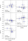 |
Fig. 3 Abundance ratios of Si, Ca, Ti, Mg, and O for the member stars in OCCASO data. Mean abundances (solid lines) and standard deviations (dotted lines) are overplotted in each panel. We have used the 7 member stars except for oxygen, which was calculated with 6 members (see text). |
3.4 Solar abundance scale
The definition of the solar abundance scale is key to calculating overall differential abundances with respect to the Sun. To define this scale we have derived Si, Ca, Ti, Mg, and O abundances in 16 solar spectra available in the Gaia FGK benchmark stars (GBS) high resolution spectral library (Blanco-Cuaresma et al. 2014b). These spectra have been acquired with different instruments and all of them have been smoothed to match the OCCASO resolution. We used the same line selection and model atmospheres as for the rest of OCCASO stars. We took the atmospheric parameters of the Sun derived in Heiter et al. (2015a).
The derived mean solar abundances for each element are: A(Si)⊙ = 7.48 ± 0.01, A(Ca)⊙ = 6.25 ± 0.02, A(Ti)⊙ = 4.91 ± 0.02, A(Mg)⊙ = 7.58 ± 0.01, and A(O)⊙ = 8.61 ± 0.04. The quoted errors are computed as the standard deviation of the 16 values. These values are consistent within 1–2σ with previous determinations of the solar abundance scale, such as Asplund et al. (2009): A(Si)⊙,A09 = 7.51 ± 0.01, A(Ca)⊙,A09 = 6.29 ± 0.02, A(Ti)⊙,A09 = 4.91 ± 0.03, A(Mg)⊙ = 7.53 ± 0.01, and A(O)⊙,A09 = 8.69 ± 0.05.
4 Comparison with the literature
Chemical abundances from high resolution spectra for NGC 6705 stars have been obtained by several authors including Gonzalez & Wallerstein (2000, GW2000); several analyses of the GES sample by Cantat-Gaudin et al. (2014b), (Magrini et al. 2014, 2015, 2017), and Tautvaišienė et al. (2015); and the latest APOGEE data releases (SDSS Collaboration 2017; Abolfathi et al. 2017). In this section we perform a star-by-star comparison for the stars in common with these studies. Finally, we compared the mean abundances that we derived for NGC 6705 with all these studies.
Gonzalez & Wallerstein (2000) analysed high-quality spectra, S∕N ≥ 85, for ten bright K giants in NGC 6705. They used the echelle spectrograph at CTIO 4m telescope (R ~ 24 000; 4200–10 000 Å) and the vacuum-sealed echelle spectrograph at APO 2.5 m telescope (R ~ 34 000; 5100–8800 Å). They derived chemical abundances using both SS and EW methods. In the framework of GES, 27 stars have been observed with UVES (R ~ 47 000; 4700–7000 Å). The spectra have been analysed independently by different teams using different methods (Smiljanic et al. 2014). Different data releases include additional data and results from different combination of the analysis methods. Finally, high resolution (R = 22 500) near infrared (H-band) spectra for several stars in the field of view of NGC 6705 have been obtained by APOGEE (Majewski et al. 2017). Atmospheric parameters and chemical abundances have been derived using the ASPCAP pipeline (García Pérez et al. 2016). There is not yet a dedicated paper to NGC 6705 from APOGEE data, for this reason, we have used the two sets of kinematical and chemical information related through SDSS data releases 13 (DR13; SDSS Collaboration 2017), and 14 (DR14; Abolfathi et al. 2017). Aside from the new data acquired between the two data releases, there are several changes in the data analysis of DR14 which include a new normalization scheme and a different treatment of the microturbulence (see Holtzman et al. 2017, for details).
4.1 Star-by-star comparison of stellar parameters
In total we have eight stars in common with GW2000, six stars with GES and three with APOGEE. In Fig. 4, we compare the values of Teff (top), log g (middle), and [Fe/H] (bottom) derived by the different authors with those obtained here. For each parameter, the mean differences and standard deviations between each sample and OCCASO are listed in Table 6 for an exhaustive comparison.
In each data release APOGEE provides two different sets of abundance values namely uncalibrated and calibrated, respectively.Uncalibrated values are those obtained directly by ASPCAP and used to perform the abundance analysis. The calibrated ones are derived using an empirical relation obtained from a sample of well characterized stars in the literature asa function of temperature, gravity and metallicity (see Nidever et al. 2015 for details). This relation is different in the different data releases. The two sets of values are significantly different, specially in log g, for which the uncalibrated ones yield large differences with OCCASO. We have limited our comparison to the calibrated parameters.
From the offsets and spreads found comparing OCCASO with the different authors in the literature we can draw some conclusions:
-
In general, Teff shows mild offsets and dispersions, that agree with the observational errors. However, as can be observed in Fig. 4, GW2000 values show a spread of 219 K, outside their large uncertainties of ~150 K. Moreover, they show a systematic trend: positive differences are observed for stars with Teff > 4700 K while for cooler stars the differences have opposite sign.
-
log g in GESiDR1 is on average 0.12 dex higher than in OCCASO, while in GESiDR2/3 and GESiDR4 show quite a good agreement with the values obtained by OCCASO. APOGEE derives larger surface gravities by 0.21 and 0.28 dex, in DR13 and DR14, respectively. This discrepancy for APOGEE log g values has already been reported in the literature (e.g. Holtzman et al. 2015). Finally, GW2000 yields a mean difference of 0.15 dex but again with a large dispersion of 0.65 dex. This may be explained by their large uncertainties in the log g determination of ~0.4 dex.
-
Except for GESiDR2/3 the [Fe/H] values of all the samples are in good agreement with the OCCASO ones even for GW2000, and in spite of the Teff and log g differences discussed above. The GESiDR2/3 values differ also with the other GES samples. The sets that are most similar to OCCASO results and with less dispersion are those of APOGEE and GESiDR4.
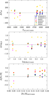 |
Fig. 4 Star-by-star comparison of OCCASO results for Teff , log g and [Fe/H] with previous high-resolution studies: APOGEE (SDSS Collaboration 2017; Abolfathi et al. 2017), GES (Magrini et al. 2014, 2017; Tautvaišienė et al. 2015), and Gonzalez & Wallerstein (2000). Differences are in the direction OCCASO-literature. Mean differences are listed in Table 6. |
Mean differences and standard deviations in atmospheric parameters and iron abundances between OCCASO (EW) and literature for the five references that have studied NGC 6705 with high-resolution spectroscopy.
4.2 Cluster mean abundances from literature
In this section we compare our mean abundances with those derived by the studies presented above. For all these comparisonswe have used the mean values and uncertainties obtained by each of them.
In the case of APOGEE, we retrieve stars in a radius of 16 arcmin around the cluster centre and with radial velocities in the range 32 < vr < 38 km s−1. This range has been selected from the analysis of OCCASO radial velocities in Paper I. We have rejected stars with radial velocity uncertainty larger than 0.5 km s−1 since they are potential spectroscopic binaries (Nidever et al. 2015). Since APOGEE Ti abundances are less reliable, we have excluded this element from our comparison (see Hawkins et al. 2016 for a detailed discussion). We have also excluded stars with Fe, Si, Ca, Mg, and O abundances discrepant with respect of the bulk of the cluster. We obtained a total of 11 potential member stars from the two data releases.
In Table 7, we list cluster mean abundance determinations by the cited studies in comparison with OCCASO results:
-
There is a very good agreement between the abundances obtainedhere and those derived by GW2000 in spite of the largeuncertainties involved in their analysis and the large differences in temperature and gravity discussed in the previous section.
-
In the case of APOGEE, there is a good agreement for [Fe/H] values. [Si/Fe] and [Ca/Fe] are slightly lower in APOGEE but the differences are well within the uncertainties. However, there is a difference in Mg of ~0.20 dex, and in O of 0.18 and 0.28 dex with APOGEE DR13 and DR14, respectively. We note that APOGEE retrieves O abundances from molecules, mainly CO and OH, while we used the forbidden [O I] atomic line.
-
In the case of GES, [Fe/H] in iDR1 and iDR4 are slightly lower than in the case of OCCASO but still within the uncertainties, but in iDR2/3 it is lower by 0.17 dex. In general, the values obtained by GES are always lower than those derived by OCCASO, except for [Mg/Fe] in iDR1 and iDR4, and [O/Fe] in iDR2/3, which is an interactive SS determination by Tautvaišienė et al. (2015).
To summarize, GW2000 shows an [α/Fe] enhancement similar to those derived in OCCASO. The same is true for APOGEE if we exclude Mg and O from the analysis. This behaviour is not observed in the case of GES except for [Mg/Fe] and [O/Fe] in iDR2/3 (Tautvaišienė et al. 2015; Magrini et al. 2015). Magrini et al. (2015), based on 27 stars, reported a high mean [α/Fe] with respect to chemical evolution models. They conclude that it is genuine, and they explore the possibility that this cluster has suffered from the effect of a local enrichment by a supernova type II.
Mean iron and α-element abundance calculated in this study: using OCCASO results (using 6 or 7 member stars, depending on the chemical species), and usingAPOGEE DR13 and DR14 results from SDSS Collaboration (2017); Abolfathi et al. (2017, 11 member stars).
5 Orbit computation
We studied whether the peculiarity in α element abundances shown by this OC could be partly explained by a very different birth and current Galactocentric radii (Sellwood & Binney 2002) (i.e. born in the inner Galaxy nearthe bar and then migrated outwards, see Sect. 1). To check that, we reconstructed the orbit of the cluster and integrated it backwards until the time of birth. To do so one basically needs: age, 3D position (l, b, and heliocentric distance d), 3D velocity (proper motions and radial velocity μacos δ, μδ , vr), and to assume a certain gravitational potential for the Milky Way2 . We used a gravitational potential that includes the Galactic bar and spiral arms resembling those of the Milky Way: a prolate bar from Pichardo et al. (2004), and the spiral arms from the PERLAS model in Pichardo et al. (2003). We refer to the cited references for details of the model and the parameters that best fit the Milky Way.
This method can carry large uncertainties: (i) errors coming from the assumed distances, motions and age; (ii) inaccuracies on the assumed model of the gravitational potential (e.g. axisymmetric, featuring the bar and/or spiral arms), and the free parameters involved in them; and (iii) for the old OCs the assumption of a static potential is not a correct approximation taking into account that typical pattern speeds of the dynamic structures can change in few Gyr. Since NGC 6705 is young, the uncertainties that come from assuming a static potential when integrating back the orbit are small.
In this section, we examine in detail the propagation of errors in the assumed motions, distance, and age. We also quantify the uncertainties that come from the choice of the model.
We used three sets of proper motions and distances specified in Table 8 to compute the orbits. Data1 uses the mean of eight stars from TGAS data (Cantat-Gaudin et al. 2018), data2 uses proper motions and distances from Dias et al. (2002), data3 uses the mean of 32 stars (Casamiquela et al. 2017b) from TGAS. In all cases we adopt vr = 34.5 ± 1.7 km s−1 (result from Paper I), and the age 316 ± 50 Myr (derived by Cantat-Gaudin et al. 2014b). For each dataset we sweep 91 different model parameters of the gravitational potential. We have explored values of: spiral arms mass (0, 0.03, 0.05 in units of disc mass, 8.56 × 10¹⁰ M⊙), spiral arms pattern speed (15, 20, 30 kms−1 kpc−1), mass of the bar (0, 0.6, 0.8 in units of bulge mass, 1.41 × 10¹⁰ M⊙), bar pattern speed (36, 46, 56 km s−1 kpc−1) and bar orientation respect to the Sun (20, 40 deg). For each model and set of input parameters we performed 100 realizations of the orbit integration assuming Gaussian errors in the motions, distance and age Fig. 5.
The results are:
-
1.
Each run of a model has a distribution of possible orbits given the assumed errors. An example for one of the models3 is plotted in, where we show the distribution of the current and birth radii, the minimum and maximum radius of the orbits. Here, the median and standard deviation of birth radius are 7.0 ± 0.7, 7.8 ± 2.5, 7.4 ± 0.8 kpc for data1, data2 and data3, respectively. In the three cases this model predicts that the cluster was born slightly outwards or almost at the current radius. The current radii computed for each datasets are very similar: 6.9 ± 0.2, 6.9 ± 0.1, 7.1 ± 0.2 kpc for data1, data2 and data3, respectively. Results of data1 and data3 are very similar, since the source of distance and proper motions is the same, though different membership selection make the birth radius differ by 0.2 kpc. Data2 results for birth, minimum and maximum radii are quite different, and they also show a larger spread and longer tails, because the errors are larger.
-
2.
The distribution of birth radius given by the 91 models and the three datasets are plotted in. It is seen that the three determinations of proper motions and distance lead to a significant difference in the computed orbits, and in particular in the radius at birth. We list the mean values of RGC,birth in Table 8. In the case of data1, in 66% of the models the radius at birth is between 6.9 < RGC,birth < 7.2 kpc (1σ from the median). For data2 60% of the cases lie within 1σ, 7.8 < RGC,birth < 8.0 kpc. In the case of data3 we obtain 7.3 < RGC,birth < 7.6 kpc in 63% of the models.
From those results, which take into account different models of the gravitational potential, different sources of the data and errors in the proper motions, radial velocity, distance and age, we can conclude that the Galactocentric radius at birth of NGC 6705 is between 6.8 < RGC,birth < 8.9 kpc. Since we have lower errors for data1 and data3, we can say that with high probability it would be between 5.4 < RGC,birth < 7.5 kpc, slightly inside the solar radius. Taking into account all the models and error realizations the birth radius is lower than 5 kpc in only 0.98%, 1.40%, 0.13% of the cases for data1, data2, and data3, respectively Fig. 6.
Three datasets of distances and proper motions, assumed in the computation of the birth radius.
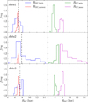 |
Fig. 5 Distributions of current and birth radii (left), and the maximum and minimum orbit radius (right), given by 100 realizations of the one of the models of the gravitational potential (see text). Each row shows the results for the three datasets specified in Table 8. The median birth radius is indicated with a dashed vertical line. |
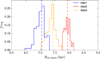 |
Fig. 6 Normalized distribution of the birth radius of the orbits given by 91 different models of the gravitational potential, and the three datasets of assumed observational parameters in Table 8. The median values of birth radius are plotted as vertical dashed lines. |
6 Discussion
From the results of OCCASO data in Sect. 3 we see that this cluster shows a clear overabundance in α elements: Si, Mg, and O show an enhancement of 0.13± 0.05, 0.14± 0.07, and 0.17 ± 0.07 respectively.Ca and Ti show more moderate values of 0.06± 0.05 and 0.03± 0.03, respectively.From comparison with other high-resolution studies (Sect. 4, Table 7): APOGEE finds similar values of [Fe/H] and [Si/Fe] as in OCCASO; in the different GES data releases a similar enhancement is derived in Si (iDR1), Mg and O (iDR2/3); and GW2000 finds mainly the same values of [Fe/H], [Si/Fe], [Ca/Fe] and [Ti/Fe]. Our resolution is much higher (R ~ 65 000–85 000) than in all previous studies, and this plays a major role when analysing spectra of metal-rich stars. On the other hand, as discussed by Magrini et al. (2015) for the GES results of this cluster, the α-enhancement in Si and Mg is genuine and not due to NLTE effects.
The literature is contradictory in the abundances of the different elements, but our results point towards a young metal-rich and α-enhanced OC, at least in some of the α-elements. Indeed, different enhancement levels for different α elements are expected on nucleosynthetic grounds, because the contribution of thermonuclear SN Type Ia to Si and Ca is expected to be more pronounced than for O or Mg (at least in standard SNIa models, e.g. Iwamoto et al. 1999, with small amounts of unburned material). This is exactly what our measurements seems to imply, with [O/Fe] > [Mg/Fe] > [Si/Fe] or [Ca/Fe], thus suggesting a protocluster cloud polluted with a larger fraction of type II SNe/type Ia SNe than the typical local gas.
As stated in Sect. 1 this feature is seen in some samples of field stars. Unlike the stars analysed by Chiappini et al. (2015), where the age has been inferred from the measurement of the mass (via the combination of seismic and spectroscopic information), and hence could be affected by later mass accretion or even merger in case of binary stars, the cluster age is much more robust. In the latter case, there is no doubt that the cluster is young, and its age is determined with unquestionable precision and accuracy, with an uncertainty of 50 Myr. Hence, this is a genuine young-alpha rich object, and could give some support to the claim of Chiappini et al. (2015) and Martig et al. (2015) that some of their stars could be indeed young, and that the evolved blue-straggler scenario (Jofré et al. 2016; Yong et al. 2016) does not explain the whole picture. In addition, the fact that NGC 6705 is located in the thin disc also supports the idea that the young α rich stars found in CoRoT inner-disc field could be thin disc stars despite their current position above the plane (z ~−300 pc).
Chiappini et al. (2015) argued, by computing the guiding radii of their analysed stars, that they find a preferential location towards the inner Galaxy, thus giving support to the idea that these stars have a common origin near the Galactic bar. From the results in Sect. 5, we see that the cluster was probably born roughly inside the solar radius, but far from the bar.
On the other hand, Magrini et al. (2015) attempts to explain this peculiarity comparing this cluster with the high-α metal-rich population (HAMR) found first by Adibekyan et al. (2011) and later confirmed by several authors. Comparing with simulations it is plausible for HAMR stars to be extreme migrators born in the inner bulge (R < 2 kpc) and that have migrated towards the solar neighbourhood (Adibekyan et al. 2013). In comparison with this cluster, the age of the HAMR stars is in general much older (in mean older than thin disc stars by about 3 Gyr).
Again, after our orbit analysis for NGC 6705 it seems unlikely that it has a common origin as the HAMR stars, so to be born in the very inner Galaxy. Of course, there are other effects that we are not taking into account in this type of analysis, such as diffusion by giant molecular clouds, transient spiral arms (Roškar et al. 2012) or resonance coupling between bar and spiral arms (Minchev & Famaey 2010), that can make the cluster migrate. But the young age of this cluster makes this option highly improbable.
There are other explanations that could apply in this case, such as a local self-enrichment by SN type II in a giant molecular cloud proposed by Magrini et al. (2015). Under their calculations an enrichment of more than 0.1 dex in [Mg/Fe], [O/Fe], and [Si/Fe] could be reached due to an SN type II explosion in the mass range 15–18 M⊙.
7 Conclusions
We have performed an abundance analysis of Fe, Si, Ca, Ti, Mg, and O from high-resolution spectroscopic data. First, we have derived abundances from seven (probable) members of NGC 6705 from OCCASO spectra. We compare results with those of APOGEE DR13 and DR14 for Ca, Si, Mg, and O. Finally, a comparison is shown among OCCASO and the different data releases of GES and APOGEE.
According to OCCASO results this OC is metal rich ([Fe/H] = 0.17 ± 0.04, Paper II) and it shows a clear α-enhancement in Si, Mg and O, and a mild enhancement above the errors in Ca and Ti. The mean [Fe/H] abundance found in OCCASO agrees very well with APOGEE, GESiDR1 and GESiDR4, it does not agree with GESiDR2/3. The mean [Si/Fe] within errors agrees with the APOGEE results and is higher than in the GES; [Ca/Fe] is higher in this work than in APOGEE and GES; [Ti/Fe] within errors agrees with GES, no results are analysed from APOGEE. The mean [Mg/Fe] agrees well within errors with GES and is higher than the results from APOGEE; the mean [O/Fe] agrees well with the precise GESiDR2 analysis result by Tautvaišienė et al. (2015), and is higher than all other results.
We have carried out a kinematic study of this cluster integrating its orbit back in time to derive its birthplace. We used three sets ofproper motions and distances, 91 assumptions for the gravitational potential free parameters, and we performed 100 realizations of each orbit assuming Gaussian errors in radial velocity, proper motion, distance and age. We conclude that the birth Galactocentric radius of NGC 6705 is probably between 6.8 < RGC,birth < 7.5 kpc. After our analysis it seems unlikely for NGC 6705 to be born near the bar, so its origin is probably different from that of the young α-enhanced stars of Chiappini et al. (2015). Another possibility could be a local self-enrichment of the giant molecular cloud by a type II SN. A more quantitative investigation should be performed to justify the latter case, so the explanation for the genuine α-enhancement of this cluster is still open.
Acknowledgments
We thank G. Tautvaišiene for refereeing this paper and for her suggestions that improved this work. This work is based on observations made with the Nordic Optical Telescope, operated by the Nordic Optical Telescope Scientific Association, and the Mercator Telescope, operated on the island ofLa Palma by the Flemish Community, both at the Observatorio del Roque de los Muchachos, La Palma, Spain, of the Instituto de Astrofísica de Canarias. This work is also based on observations collected at the Centro Astronómico Hispano Alemán (CAHA) at Calar Alto, operated jointly by the Max-Planck Institut für Astronomie and the Instituto de Astrofísicade Andalucía (CSIC). This research made use of the WEBDA database, operated at the Department of Theoretical Physics and Astrophysics of the Masaryk University, the SIMBAD database, operated at the CDS, Strasbourg, France, and the TOPCAT tool version 4.4. This work has made use of the VALD database, operated at Uppsala University, the Institute of Astronomy RAS in Moscow, and the University of Vienna. This work was supported by the MINECO (Spanish Ministry of Economy) – FEDER through grant ESP2016-80079-C2-1-R and ESP2014-55996-C2-1-R and MDM-2014-0369 of ICCUB (Unidad de Excelencia “María de Maeztu”). LC acknowledges financial support from the University of Barcelona under the APIF grant.
References
- Abolfathi, B., Aguado, D. S., Aguilar, G., et al. 2017, ApJS, submitted, [arXiv:1707.09322] [Google Scholar]
- Adibekyan, V. Z., Santos, N. C., Sousa, S. G., & Israelian, G. 2011, A&A, 535, L11 [NASA ADS] [CrossRef] [EDP Sciences] [Google Scholar]
- Adibekyan, V. Z., Figueira, P., Santos, N. C., et al. 2013, A&A, 554, A44 [NASA ADS] [CrossRef] [EDP Sciences] [Google Scholar]
- Allende Prieto, C., Lambert, D. L., & Asplund, M. 2001, ApJ, 556, L63 [NASA ADS] [CrossRef] [Google Scholar]
- Alves-Brito, A., Meléndez, J., Asplund, M., Ramírez, I., & Yong, D. 2010, A&A, 513, A35 [NASA ADS] [CrossRef] [EDP Sciences] [Google Scholar]
- Asplund, M., Grevesse, N., Sauval, A. J., & Scott, P. 2009, ARA&A, 47, 481 [NASA ADS] [CrossRef] [Google Scholar]
- Bavarsad, E. A., Sandquist, E. L., Shetrone, M. D., & Orosz, J. A. 2016, ApJ, 831, 48 [NASA ADS] [CrossRef] [Google Scholar]
- Beaver, J., Kaltcheva, N., Briley, M., & Piehl, D. 2013, PASP, 125, 1412 [NASA ADS] [CrossRef] [Google Scholar]
- Bensby, T., Feltzing, S., & Oey, M. S. 2014, A&A, 562, A71 [NASA ADS] [CrossRef] [EDP Sciences] [Google Scholar]
- Bergemann, M., Ruchti, G. R., Serenelli, A., et al. 2014, A&A, 565, A89 [NASA ADS] [CrossRef] [EDP Sciences] [Google Scholar]
- Blanco-Cuaresma, S., Soubiran, C., Heiter, U., & Jofré, P. 2014a, A&A, 569, A111 [CrossRef] [EDP Sciences] [Google Scholar]
- Blanco-Cuaresma, S., Soubiran, C., Jofré, P., & Heiter, U. 2014b, A&A, 566, A98 [CrossRef] [EDP Sciences] [Google Scholar]
- Bressan, A., Marigo, P., Girardi, L., et al. 2012, MNRAS, 427, 127 [NASA ADS] [CrossRef] [Google Scholar]
- Caffau, E., Ludwig, H.-G., Steffen, M., et al. 2008, A&A, 488, 1031 [NASA ADS] [CrossRef] [EDP Sciences] [Google Scholar]
- Cantat-Gaudin, T., Donati, P., Pancino, E., et al. 2014a, A&A, 562, A10 [NASA ADS] [CrossRef] [EDP Sciences] [Google Scholar]
- Cantat-Gaudin, T., Drew, J. E., Eisloeffel, J., et al. 2014b, A&A, 569, A17 [NASA ADS] [CrossRef] [EDP Sciences] [Google Scholar]
- Cantat-Gaudin, T., Vallenari, A., Sordo, R., et al. 2018, A&A, in press, DOI: 10.1051/0004-6361/201731251 [Google Scholar]
- Casamiquela, L., Carrera, R., Jordi, C., et al. 2016, MNRAS, 458, 3150 [NASA ADS] [CrossRef] [Google Scholar]
- Casamiquela, L., Carrera, R., Blanco-Cuaresma, S., et al. 2017a, MNRAS, 470, 4363 [NASA ADS] [CrossRef] [Google Scholar]
- Casamiquela, L., Jordana, N., Balaguer-Nunez, L., et al. 2017b, A&A, submitted [Google Scholar]
- Chiappini, C., Anders, F., Rodrigues, T. S., et al. 2015, A&A, 576, L12 [NASA ADS] [CrossRef] [EDP Sciences] [Google Scholar]
- Dias, W. S., Alessi, B. S., Moitinho, A., & Lépine, J. R. D. 2002, A&A, 389, 871 [NASA ADS] [CrossRef] [EDP Sciences] [Google Scholar]
- Fuhrmann, K. 2011, MNRAS, 414, 2893 [NASA ADS] [CrossRef] [Google Scholar]
- Fulbright, J. P., McWilliam, A., & Rich, R. M. 2007, ApJ, 661, 1152 [NASA ADS] [CrossRef] [Google Scholar]
- García Pérez, A. E., Allende Prieto, C., Holtzman, J. A., et al. 2016, AJ, 151, 144 [CrossRef] [Google Scholar]
- Gilmore, G., Randich, S., Asplund, M., et al. 2012, The Messenger, 147, 25 [NASA ADS] [Google Scholar]
- Gonzalez, G., & Wallerstein, G. 2000, PASP, 112, 1081 [NASA ADS] [CrossRef] [Google Scholar]
- Grevesse, N., Asplund, M., & Sauval, A. J. 2007, Space Sci. Rev., 130, 105 [NASA ADS] [CrossRef] [Google Scholar]
- Gustafsson, B., Edvardsson, B., Eriksson, K., et al. 2008, A&A, 486, 951 [NASA ADS] [CrossRef] [EDP Sciences] [Google Scholar]
- Hawkins, K., Masseron, T., Jofré, P., et al. 2016, A&A, 594, A43 [NASA ADS] [CrossRef] [EDP Sciences] [Google Scholar]
- Haywood, M., Di Matteo, P., Lehnert, M. D., Katz, D., & Gómez, A. 2013, A&A, 560, A109 [NASA ADS] [CrossRef] [EDP Sciences] [Google Scholar]
- Heiter, U., Jofré, P., Gustafsson, B., et al. 2015a, A&A, 582, A49 [NASA ADS] [CrossRef] [EDP Sciences] [PubMed] [Google Scholar]
- Heiter, U., Lind, K., Asplund, M., et al. 2015b, Phys. Scr., 90, 054010 [CrossRef] [Google Scholar]
- Holtzman, J. A., Shetrone, M., Johnson, J. A., et al. 2015, AJ, 150, 148 [NASA ADS] [CrossRef] [Google Scholar]
- Holtzman, J. A., Hasselquist, S., Johnson, J., et al. 2017, in AAS Meeting Abstr., 229, 216.01 [Google Scholar]
- Iwamoto, K., Brachwitz, F., Nomoto, K., et al. 1999, ApJS, 125, 439 [NASA ADS] [CrossRef] [MathSciNet] [Google Scholar]
- Jofré, P., Jorissen, A., Van Eck, S., et al. 2016, A&A, 595, A60 [CrossRef] [EDP Sciences] [Google Scholar]
- Johansson, S., Litzén, U., Lundberg, H., & Zhang, Z. 2003, ApJ, 584, L107 [NASA ADS] [CrossRef] [Google Scholar]
- Kurucz, R. L. 2005, Mem. Soc. Astron. It. Suppl., 8, 14 [Google Scholar]
- Kurucz, R. L. 2010, On-line database of observed and predicted atomic transitions, http://kurucz.harvard.edu/atoms/2808/gf2808.lines [Google Scholar]
- Magrini, L., Randich, S., Romano, D., et al. 2014, A&A, 563, A44 [NASA ADS] [CrossRef] [EDP Sciences] [Google Scholar]
- Magrini, L., Randich, S., Donati, P., et al. 2015, A&A, 580, A85 [NASA ADS] [CrossRef] [EDP Sciences] [Google Scholar]
- Magrini, L., Randich, S., Kordopatis, G., et al. 2017, A&A, 603, A2 [CrossRef] [EDP Sciences] [Google Scholar]
- Majewski, S. R., Schiavon, R. P., Frinchaboy, P. M., et al. 2017, AJ, 154, 94 [NASA ADS] [CrossRef] [Google Scholar]
- Martig, M., Rix, H.-W., Silva Aguirre, V., et al. 2015, MNRAS, 451, 2230 [NASA ADS] [CrossRef] [Google Scholar]
- Mathieu, R. D., Latham, D. W., Griffin, R. F., & Gunn, J. E. 1986, AJ, 92, 1100 [NASA ADS] [CrossRef] [Google Scholar]
- Matteucci, F., 2001, The chemical evolution of the Galaxy, Astrophys. Space Sci. Lib., 253, The chemical evolution of the Galaxy, [Google Scholar]
- McNamara, B. J., Pratt, N. M., & Sanders, W. L. 1977, A&AS, 27, 117 [NASA ADS] [Google Scholar]
- Mermilliod, J. C., Mayor, M., & Udry, S. 2008, A&A, 485, 303 [NASA ADS] [CrossRef] [EDP Sciences] [Google Scholar]
- Miglio, A., Chiappini, C., Morel, T., et al. 2013, MNRAS, 429, 423 [NASA ADS] [CrossRef] [Google Scholar]
- Minchev, I., & Famaey, B. 2010, ApJ, 722, 112 [NASA ADS] [CrossRef] [Google Scholar]
- Mucciarelli, A., Pancino, E., Lovisi, L., Ferraro, F. R., & Lapenna, E. 2013, ApJ, 766, 78 [NASA ADS] [CrossRef] [Google Scholar]
- Nidever, D. L., Holtzman, J. A., Allende Prieto, C., et al. 2015, AJ, 150, 173 [NASA ADS] [CrossRef] [Google Scholar]
- Pichardo, B., Martos, M., Moreno, E., & Espresate, J. 2003, ApJ, 582, 230 [NASA ADS] [CrossRef] [Google Scholar]
- Pichardo, B., Martos, M., & Moreno, E. 2004, ApJ, 609, 144 [NASA ADS] [CrossRef] [Google Scholar]
- Raskin, G., van Winckel, H., Hensberge, H., et al. 2011, A&A, 526, A69 [NASA ADS] [CrossRef] [EDP Sciences] [Google Scholar]
- Reid, M. J., Menten, K. M., Brunthaler, A., et al. 2014, ApJ, 783, 130 [NASA ADS] [CrossRef] [Google Scholar]
- Roškar, R., Debattista, V. P., Quinn, T. R., & Wadsley, J. 2012, MNRAS, 426, 2089 [NASA ADS] [CrossRef] [Google Scholar]
- Santos, Jr. J. F. C., Bonatto, C., & Bica, E. 2005, A&A, 442, 201 [NASA ADS] [CrossRef] [EDP Sciences] [Google Scholar]
- Sbordone, L., Bonifacio, P., Castelli, F., & Kurucz, R. L. 2004, Mem. Soc. Astron. It. Suppl., 5, 93 [Google Scholar]
- SDSS Collaboration, Albareti, F. D., Allende Prieto, C et al. 2017, ApJS, 233, 25 [CrossRef] [Google Scholar]
- Sellwood, J. A., & Binney, J. J. 2002, MNRAS, 336, 785 [NASA ADS] [CrossRef] [Google Scholar]
- Smiljanic, R., Korn, A. J., Bergemann, M., et al. 2014, A&A, 570, A122 [NASA ADS] [CrossRef] [EDP Sciences] [Google Scholar]
- Stetson, P. B., & Pancino, E. 2008, PASP, 120, 1332 [NASA ADS] [CrossRef] [Google Scholar]
- Sung, H., Bessell, M. S., Lee, H.-W., Kang, Y. H., & Lee, S.-W. 1999a, MNRAS, 310, 982 [NASA ADS] [CrossRef] [Google Scholar]
- Sung, H., Bessell, M. S., Lee, H.-W., Kang, Y. H., & Lee, S.-W. 1999b, MNRAS, 310, 982 [Google Scholar]
- Tautvaišienė, G., Drazdauskas, A., Mikolaitis, S., et al. 2015, A&A, 573, A55 [CrossRef] [EDP Sciences] [Google Scholar]
- Telting, J. H., Avila, G., Buchhave, L., et al. 2014, Astron. Nachr., 335, 41 [NASA ADS] [CrossRef] [Google Scholar]
- Yong, D., Casagrande, L., Venn, K. A., et al. 2016, MNRAS, 459, 487 [NASA ADS] [CrossRef] [Google Scholar]
Other parameters are needed, including Sun position and velocity: R0 = 8.34 kpc, (U, V, W)0 = (10.7, 15.6, 8.9) km s−1, and Galactic rotation 240 km s−1 (Reid et al. 2014).
All Tables
Atomic parameters (oscillator strength and excitation potential) and references for the two Mg lines used, the O forbidden line, and the Ni blend.
Absolute abundances per spectrum of the two Mg lines used, and the O forbidden line.
Mean differences and standard deviations in atmospheric parameters and iron abundances between OCCASO (EW) and literature for the five references that have studied NGC 6705 with high-resolution spectroscopy.
Mean iron and α-element abundance calculated in this study: using OCCASO results (using 6 or 7 member stars, depending on the chemical species), and usingAPOGEE DR13 and DR14 results from SDSS Collaboration (2017); Abolfathi et al. (2017, 11 member stars).
Three datasets of distances and proper motions, assumed in the computation of the birth radius.
All Figures
|
Fig. 1 Colour-magnitude diagram with the photometry from Sung et al. (1999b). Target stars are marked with red crosses.A PARSEC isochrone of age 316 Myr and Z = 0.019 shifted by V − MV = 11.45 (d = 1950 pc) and E(B − V) = 0.40 (Cantat-Gaudin et al. 2014b) is overplotted. |
| In the text | |
|
Fig. 2 Derived Teff and log g in Paper II. Grey points are the values of the stars observed with both FIES and HERMES. For these stars we also plot the mean values (in black). The same isochrone as in Fig. 1 is overplotted. |
| In the text | |
|
Fig. 3 Abundance ratios of Si, Ca, Ti, Mg, and O for the member stars in OCCASO data. Mean abundances (solid lines) and standard deviations (dotted lines) are overplotted in each panel. We have used the 7 member stars except for oxygen, which was calculated with 6 members (see text). |
| In the text | |
|
Fig. 4 Star-by-star comparison of OCCASO results for Teff , log g and [Fe/H] with previous high-resolution studies: APOGEE (SDSS Collaboration 2017; Abolfathi et al. 2017), GES (Magrini et al. 2014, 2017; Tautvaišienė et al. 2015), and Gonzalez & Wallerstein (2000). Differences are in the direction OCCASO-literature. Mean differences are listed in Table 6. |
| In the text | |
|
Fig. 5 Distributions of current and birth radii (left), and the maximum and minimum orbit radius (right), given by 100 realizations of the one of the models of the gravitational potential (see text). Each row shows the results for the three datasets specified in Table 8. The median birth radius is indicated with a dashed vertical line. |
| In the text | |
|
Fig. 6 Normalized distribution of the birth radius of the orbits given by 91 different models of the gravitational potential, and the three datasets of assumed observational parameters in Table 8. The median values of birth radius are plotted as vertical dashed lines. |
| In the text | |
Current usage metrics show cumulative count of Article Views (full-text article views including HTML views, PDF and ePub downloads, according to the available data) and Abstracts Views on Vision4Press platform.
Data correspond to usage on the plateform after 2015. The current usage metrics is available 48-96 hours after online publication and is updated daily on week days.
Initial download of the metrics may take a while.