| Issue |
A&A
Volume 610, February 2018
|
|
|---|---|---|
| Article Number | A25 | |
| Number of page(s) | 14 | |
| Section | Planets and planetary systems | |
| DOI | https://doi.org/10.1051/0004-6361/201731407 | |
| Published online | 19 February 2018 | |
Visible spectroscopy of the Sulamitis and Clarissa primitive families: a possible link to Erigone and Polana★
1
Instituto de Astrofísica de Canarias (IAC),
C/vía Láctea s/n,
38205
La Laguna,
Tenerife, Spain
e-mail: damog@iac.es
2
Departamento de Astrofísica, Universidad de La Laguna,
38205
La Laguna,
Tenerife, Spain
3
Observatório Nacional, Coordenação de Astronomia e Astrofísica,
20921-400
Rio de Janeiro, Brazil
4
GTC Project Office,
38205
La Laguna,
Tenerife, Spain
5
Physics Department, University of Central Florida,
PO Box 162385,
Orlando,
FL
32816-2385, USA
6
Florida Space Institute, University of Central Florida,
Orlando,
FL
32816, USA
Received:
20
June
2017
Accepted:
5
October
2017
The low-inclination (i < 8∘) primitive asteroid families in the inner main belt, that is, Polana-Eulalia, Erigone, Sulamitis, and Clarissa, are considered to be the most likely sources of near-Earth asteroids (101955) Bennu and (162173) Ryugu. These two primitive NEAs will be visited by NASA OSIRIS-REx and JAXA Hayabusa 2 missions, respectively, with the aim of collecting samples of material from their surfaces and returning them back to Earth. In this context, the PRIMitive Asteroid Spectroscopic Survey (PRIMASS) was born, with the main aim to characterize the possible origins of these NEAs and constrain their dynamical evolution. As part of the PRIMASS survey we have already studied the Polana and Erigone collisional families in previously published works. The main goal of the work presented here is to compositionally characterize the Sulamitis and Clarissa families using visible spectroscopy. We have observed 97 asteroids (64 from Sulamitis and 33 from Clarissa) with the OSIRIS instrument (0.5-0.9 μm) at the 10.4 m Gran Telescopio Canarias (GTC). We found that about 60% of the sampled asteroids from the Sulamitis family show signs of aqueous alteration on their surfaces. We also found that the majority of the Clarissa members present no signs of hydration. The results obtained here show similarities between Sulamitis-Erigone and Clarissa-Polana collisional families.
Key words: minor planets, asteroids: general / methods: data analysis / techniques: spectroscopic
The reduced spectra are only available at the CDS via anonymous ftp to cdsarc.u-strasbg.fr (130.79.128.5) or via http://cdsarc.u-strasbg.fr/viz-bin/qcat?J/A+A/610/A25
© ESO 2018
1 Introduction
Primitive asteroids are characterized by dark surfaces dominated by carbon compounds and are associated with carbonaceous chondrites, the most pristine meteorites in our records. These are usually composed of water-bearing minerals and organics, and so they carry the answer to the unsolved question on how water and life appeared on Earth. These life-forming materials present rather featureless spectra in visible to near-infrarred wavelengths, showing diagnostic absorption features in the 3 μm region. In particular, there is a hydration band centered around 2.7−2.9 μm and observed in infrared photometry and spectroscopy of many primitive asteroids, that is correlated with the 0.7 μm Fe2+ → Fe+3 oxidized iron absorption band observed in their visible spectra (Vilas & Gaffey 1989; Vilas 1994; Howell et al. 2011; Rivkin 2012). Aqueous alteration acts on primitive asteroids (C, B, and low albedo X-types, according to the DeMeo et al. (2009) classification scheme) by producing a low-temperature (<320 K) chemical alteration of the materials due to the presence of liquid water. This water acts as a solvent and generates hydrated materials like phyllosilicates, sulfates, oxides, carbonates, and hydroxides. Thus, the existence of hydrated materials on the surface of asteroids implies that, at some point, liquid water was present on these objects, produced by the melting of water ice by heating processes (Fornasier et al. 2014). Primitive asteroids have suffered minimal geological or thermal evolution, but have experienced an intense collisional evolution that affected their size, shape, and surface composition.
Collisional families are groups of fragments (“members”) generated by a disruptive collisional event of a larger parent body. Therefore, members of a family share similar orbital properties. Spectroscopic observations of the Vesta family (Binzel & Xu 1993) provided the first confirmation of the collisional origin of a family and since then the spectroscopic study of collisional families have steadily increased. In addition, having in mind that near-Earth asteroids (NEAs) come principally from the main asteroid belt (Bottke et al. 2002), collisional families are preferred as sources of NEAs as they generate a lot of small chunks when they are formed. Families placed near particular resonances in the main belt can effortlessly drive these chunks into the near-Earth space. Because of this, the inner asteroid belt (the region located between the ν6 resonance, near 2.15 AU, and the 3:1 mean-motion resonance with Jupiter, at 2.5 AU) is thought to be the primary source of the near Earth asteroid population (Bottke et al. 2002).
Two sample-return missions, NASA OSIRIS-REx (Lauretta et al. 2010) and JAXA Hayabusa2 (Tsuda et al. 2013) have targeted primitive NEAs: (101955) Bennu and (162173) Ryugu, respectively. These asteroids are believed to originate in the inner belt, where five possible sources have been identified: the four primitive collisional families Polana, Erigone, Sulamitis, and Clarissa, and a population of low-albedo and low-inclination background asteroids (Campins et al. 2010, 2013; Gayon-Markt et al. 2012; Bottke et al. 2015). The compositional characterization of the source regions of these two NEAs will enhance the science return of these missions.
With this objective in mind we started in 2010 a spectroscopic survey in the visible and the near-infrared to characterize the primitive collisional families in the inner belt and the low-albedo background population. This is the PRIMitive Asteroid Spectroscopic Survey (PRIMASS). It includes also primitive collisional families and dynamical populations of the outer main belt, as well as other groups of primitive asteroids, like the B-types. So far we have spectroscopically observed more than 400 asteroids.
We have already published some results on the characterization of these inner belt families. Results from visible spectroscopy for the Polana-Eulalia family complex and for the Erigone family can be found in de León et al. (2016) and Morate et al. (2016) respectively, mainly obtained with the 10.4 m Gran Telescopio Canarias (GTC), located at the El Roque de los Muchachos Observatory, in the island of La Palma (Spain). Results from near-infrared spectroscopy for the Polana-Eulalia complex can be found in Pinilla-Alonso et al. (2016). These were obtained using both the Telescopio Nazionale Galileo (TNG) and the NASA Infrared Telescope Facility (IRTF). We have also published results on the Hilda and Cybele groups in the outer main belt (De Prá et al. 2017).
To continue with our PRIMASS survey, we have observed and characterized the Sulamitis and Clarissa families by means of visible spectroscopy. These are the smallest families of the low-inclination (i < 8°) primitive families in the inner belt. We have carried out our study using visible spectra obtained with the GTC during the semesters 2015A, 2015B, and 2016A (January 2015–August 2016), following similar procedures for the data acquisition, reduction, and compositional analysis as those described in Morate et al. (2016). Details on the observations and on the data reduction are presented in Sect. 2. In Sect. 3 we present the analysis of the data, including taxonomical classification, computation of spectral slopes and analysis of aqueous alteration. In Sect. 4 we discuss the obtained results, and the conclusions are summarized in Sect. 5.
2 Observations and data reduction
The asteroids observed within this study have been selected using the dataset of families from Nesvorny (2015) in the Small Bodies Node of the NASA Planetary Data System. This dataset contains asteroid dynamical family memberships for 122 families calculated from synthetic proper elements, including high-inclination families, computed by David Nesvorný (Nesvorný et al. 2015) using his code based on the Hierarchical Clustering Method (HCM) as described in Zappala et al. (1990) and Zappala & Cellino (1994). The dataset also provides values for the absolute magnitude of the asteroids (Hv), as well as their synthetic proper elements used to compute family membership. According to this dataset, the Sulamitis and Clarissa families have 303 and 179 members, respectively. Table B.2 shows the orbital and physical information on the asteroids studied in this work, including proper semi-major axis (a), eccentricity (e), inclination (i), and absolute magnitude. Whenever available, we included the diameter (D) and geometric albedos (pV) extracted from the NEOWISE database (Mainzer et al. 2016).
Sulamitis and Clarisa collisional families are classified as primitive ones based on the information regarding visible albedo (and taxonomical classification of a few) of their members. From the 174 members of the Sulamitis family having visible albedo determinations, 170 show values of pV < 0.1. In the case of the Clarissa family, a total of 68 objects have pV determined, and 67 of them have also pV < 0.1. Selecting just objects with pV < 0.1 would be excessively conservative, leaving us without observable targets at some nights of the semesters (see Sect. 2.1 for more details). Therefore, our only constraint was the apparent visual magnitude of the objects, being in the range 18 < mV < 21, observing objects with and without a priori information on their albedo. An exception to this constraint are asteroids (752) Sulamitis and (302) Clarissa, which are the largest (and brightest) members of the families, and their expected parent bodies.
2.1 Observations
A total of 97 low-resolution visible spectra were obtained for the asteroids in the Sulamitis and Clarissa families (64 and 33 objects, respectively), using the Optical System for Imaging and Low Resolution Integrated Spectroscopy (OSIRIS) camera spectrograph (Cepa et al. 2000; Cepa 2010) at the 10.4 m GTC, located at the El Roque de los Muchachos Observatory (ORM) in La Palma, Canary Islands, Spain. See Sect. 2.1 in Morate et al. (2016) for further information about the OSIRIS instrument and specifications.
The instrument configuration and the observational procedure are the same that we used for the observations in Morate et al. (2016), except for the use of a 2.5″-width slit, instead of the 5″-width slit used in the previous work. Observational details are shown in Table B.1, including asteroid number, date of observation, starting time of the first exposition, exposure time, and visible magnitude (mV) at the moment of the observation. We also include the solar analog stars used to obtain the reflectance spectra.
Observations were done in service mode within GTC programs GTC18-15A, GTC48-15B, and GTC15-16A, on different nights from January 2015 to August 2016. Given the fact that the program is classified as a filler within the GTC schedule, night qualities were rather variable, covering a wide range of different weather conditions. The goal of these filler programs is to obtain high S/N spectra for targets that are relatively bright for a 10 m-class telescope in non-optimal weather conditions. These would include high seeing values (up to 2.0″), full moon, or some cirrus coverage. Because of this, spectra quality might vary from one night to another.
In addition, we obtained three spectra of (752) Sulamitis using the Intermediate Dispersion Spectrograph (IDS) at the 2.5 m Isaac Newton Telescope (INT), also located at the ORM in La Palma, as part of program C97 (2015), on July 22, 2015. The IDS instrument was used with a 4096 × 2048 pixels RED+2 CCD detector, having a scale plate of 0.44″/pixel, and a total of 2200 unvignetted pixels. The spectra were obtained using the R150V grism, which produces a dispersion of 4.03 Å/pixel, for a slit of 1.0″, covering the spectral range from 4000–10 000 Å. The R150V grism was used in combination of a 1.5″ slit. The observational procedure was the same as the one we used for the observations with the OSIRIS instrument at the GTC, described above.
2.2 Data reduction
To reduce the spectroscopic data obtained with the GTC we used a similar procedure as that described inMorate et al. (2016), using our own developed pipeline combining standard IRAF1 tasks and some Python routines. The process included bias and flat-field correction of the 2D-images, sky background subtraction and 1D-spectra extraction, and wavelength calibration using Xe+Ne+HgAr lamps. We used the same pipeline to reduce the INT spectrum of (752) Sulamitis.
To correct for telluric absorptions and to obtain relative reflectance spectra, at least one solar analog star from the Landolt catalog (Landolt 1992) was observed each night. Whenever possible, more than one solar analog star was observed in order to improve the quality of the final spectra and to minimize potential variations in spectral slope introduced by the use of one single star. In those cases, the reflectance spectra obtained for the asteroids against each solar analog were averaged to obtain the final result. These stars were observed using the same spectral configuration as that for the asteroids, and at similar airmass. The list of solar analogs used in this study is shown in Table 1, including an identification number ID (the same as the one appearing in the last column of Table B.1), their right ascension (α) and declination (δ), and their visible magnitude (V). From the total of 36 observation nights, in 16 of them more than one solar analog was observed. We computed the possible fluctuations in spectral slopes on these nights due to the use of different stars. The largest value we obtained for the slope variation was 0.8%/1000 Å. As we will explain in the next section, this will be the dominating error regarding the asteroid spectral slopes. The resulting spectra were normalized to unity at 0.55 μm (this is the central wavelength of the V Johnson filter, which is widely used as reference for normalization in the visible) and are shown in Figs. A.1 and A.2.
Right ascension, declination, and visible magnitude for the solar analog stars used to obtain the reflectance spectra of the observed asteroids.
3 Analysis and results
We have performed in-depth analysis on the obtained spectra. In the following sections we will describe how did we determine the taxonomy ofthe observed asteroids, how is the Yarkovsky effect affecting the family members, and, for the primitive objects in the sample, we have computed the spectral slopes, and we have looked for the absorption feature at 0.7 microns related to hydrated minerals on the surface of the asteroids. Finally, we compared our observations of (752) Sulamitis with the spectral data of this asteroid present in the literature.
3.1 Taxonomy determination
Once the data was reduced, we performed a taxonomic classification of the resulting spectra using the M4AST2 online tool. The procedure used by the M4AST tool to classify asteroid spectra is summarized in Popescu et al. (2012) and is based on the DeMeo et al. (2009) taxonomy, an extension to the near-infrared of the Bus & Binzel (2002) taxonomy in the visible. Most of the classes in the DeMeo et al. (2009) overlap the ones in Bus & Binzel (2002), but, since we are working only with visible spectra (0.5–0.9 μm), we have checked individually those cases in which the taxonomical classes were exclusive to the DeMeo et al. (2009) taxonomy and classified them according to Bus & Binzel (2002).
To obtain robust results, we selected the χ2 option (Bevington & Robinson 1992) available in the M4AST tool to test how well the spectra fitted to the templates. The best result was that corresponding to the smallest standard deviation. The taxonomical classification obtained for each asteroid is shown in the last column of Table B.2.
The classification procedure of the Sulamitis spectra provided a total of 32 C-type asteroids (including subclasses Ch and Cgh), 18 X-types (including one Xe-type), one B-type, seven T-types, and six objects with non-primitive classifications (three V-types, two A-types, and one Sr-type). In the case of the Clarissa family, we found 16 C-types (including one Cgh-type), five X-types, 11 B-types, and one V-type. These results are summarized in two pie charts (Fig. 1). As expected from the albedo information extracted from the NEOWISE database, the majority of the asteroids in both families belong to primitive taxonomical classes. From the seven asteroids classified as non-primitive, we found albedo information from WISE database for two of them: (70528) and (79143). Both objects are classified as V-types and have pV > 0.2, in agreement with their non-primitive nature.
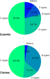 |
Fig. 1 Distribution of the taxonomical classes for the sample of 64 Sulamitis family asteroids (top panel) and the 33 Clarissa family asteroids (bottom panel) studied in this paper. The “Other” class includes all non-primitive taxonomies (S-types, V-types, and A-types). |
3.2 The Yarkovsky effect on the Sulamitis and Clarissa families
As described by Vokrouhlický et al. (2006), collisional families show signs of having experienced dynamical spreading via the Yarkovsky thermal forces (spread in values of semi-major axis). Figure 2 shows the distribution in the absolute magnitude and semi-major axis space (H, a) for the members of both families. Solid curves in this figure define the boundaries of the family, also known as the “Yarkovsky cone”, computed using the expression
 (1)
(1)
where Δa = a − ac, with ac defined as the center of the family. In practice, ac is often close to, or the same as, the semimajor axis of the largest member of the family. C is a constant, different for each family, defined in Bottke et al. (2015), where they show that C = 2.15 × 10⁻⁵ AU for the Sulamitis family, and C = 4.15 × 10⁻⁶ AU for the Clarissa family. This Yarkovsky cone is an “envelope” around the center of the family, indicating the furthest that a family member can drift as a function of its size. Objects outside this cone are likely family interlopers. In addition, objects having a different composition from that of the family, are also considered as interlopers. In the cases we are studying, there are three objects belonging to the Sulamitis family with a non-primitive taxonomy lying outside this cone (from a total of six non-primitive asteroids). Regarding the Clarissa family, the only non-primitive object observed lies outside the Yarkovksy cone. This behavior is something we would expect given the definition of the Yarkovsky envelope. However, since this definition is empirical, we can find both primitive objects outside this cone (objects that might have drifted away from the family more than expected) and non-primitive objects inside the envelope. If we suppose that the original body had an homogeneous composition, the latter would likely be spurious members, which fall inside the family because of the exclusively dynamical definition of the group.
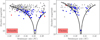 |
Fig. 2 Absolute magnitude (H) of the asteroids from the Sulamitis and Clarissa families as a function of their proper semi-major axes. Both families are shown in gray. The colored circles correspond to the objects observed in this study. Objects depicted in blue are primitive asteroids (C, X, B, T, and subclasses), while objects in red are non-primitive (A-, V-, and S-types). The family parent asteroids, (752) Sulamitis and (302) Clarissa, are represented as stars and are the largest objects in the families. |
3.3 Spectral slopes
Primitive asteroids have almost featureless, linear spectra. Therefore we started by computing their spectral slope S′, as defined by (Luu & Jewitt 1990), in the range from 0.55 to 0.90 μm, using the expression
 (2)
(2)
where d S∕dλ is the rate of change of the reflectance in the aforementioned wavelength range, and S0.55 is the reflectance at 0.55 μm. To compute S′, we applied a linear least-squares fit between 0.55 and 0.90 μm to the whole spectrum of every primitive asteroid. The values we used for d S∕d λ and S0.55 are, respectively, the slope of the aforementioned fit and its value at 0.55 microns3. S′ is measured in units of %∕1000 Å. The resulting values for the computed spectral slopes are shown in Table B.2. The variation in the slope due to the solar analog stars (see Sect. 2.2) is always larger than the 1σ standard deviation given by the linear fit. Therefore, the uncertainty in the slope will be 0.8%∕1000 Å for all cases.
Figure 3 shows the distribution of the computed slopes for several cases. In the upper-left panel we show the slope distributions for the two families studied in this paper: Sulamitis and Clarissa. We can see that the slope distributions are different, with the Sulamitis family showing redder slope on average. The upper-right panel shows the comparison between the slope distributions of the largest primitive families in the inner main belt, Polana and Erigone, as computed by de León et al. (2016) and Morate et al. (2016). Here we observe a similar behavior to that of the previous case, with the slope distribution of the Erigone family being redder than that of Polana. This led us to compare the “blue” families (Clarissa and Polana) on one panel, and the “red” families (Sulamitis and Erigone) on other panel, in an attempt to better visualize their apparent similarities. We can see in Fig. 3 that the difference between the slope distributions of Clarissa and Polana (lower-left) is considerably small, while Sulamitis and Erigone (lower-right) show very similar slope distributions. The mean values for the four slope distributions are 2.12 (Sulamitis), 1.81 (Erigone), 0.17 (Clarissa), and −0.48 (Polana) %∕1000 Å.
To quantify these similarities we run a two-sample Kolmogorov-Smirnov test (KS-test) over the two pairs of distributions (see Chap. 14 in Press 1992, and references within). We rejected the hypothesis of both samples coming from the same distribution if:
 (3)
(3)
where Dm,n is the Kolmogorov-Smirnov statistic, c(α) = 1.36 for a confidence level of α = 0.05, and m and n are the sizes of the compared samples. With these data, the critical value for the Sulamitis-Erigone test was Dcrit,Sul,Eri = 0.23, and the critical value for the Clarissa-Polana test was Dcrit,Cla,Pol = 0.29. When we run the KS-test, the results were DSul,Eri = 0.13, and DCla,Pol = 0.27. This means that we cannot reject the hypothesis of both samples coming from the same distribution in either case. Furthermore, if we compare any other pair of distributions among these four families, the results of the KS-test point out to samples coming from different distributions. Since this two-sample KS-test is used to check the difference between two one-dimensional cumulative distribution functions, we are plotting the functions for the four families in Fig. 4 for a graphical representation of this comparison.
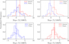 |
Fig. 3 Comparison of the spectral slope distributions of the primitive families in the inner main belt. The bin size is 0.87%/1000 Å. From left to right, top to bottom: sulamitis vs. Clarissa (this work), Polana vs. Erigone (the largest families, see Morate et al. 2016 for in-depth results), Clarissa vs. Polana, and Sulamitis vs. Erigone. Sulamitis and Erigone have been depicted in red, and Clarissa and Polana in blue. The vertical lines represent the mean values of the slope distributions. See text for more details. |
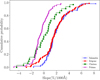 |
Fig. 4 Cumulative distribution function (CDF) of the slopes for the four primitive families of the inner main belt: Sulamitis and Clarissa (this work), Polana (de León et al. 2016), and Erigone (Morate et al. 2016). The Kolmogorov-Smirnov test compares the CDFs and gives an estimation of the differences. |
3.4 Aqueousalteration
A considerable number of main belt primitive asteroids show an absorption feature centered around 0.7 μm in their visible spectra (Vilas 1994; Fornasier et al. 1999, 2014; Carvano et al. 2003; Rivkin 2012; Morate et al. 2016), attributed to charge transfer transitions in oxidized iron, indicative of, or associated to, the presence of aqueous altered minerals on their surfaces (Vilas & Gaffey 1989; Vilas 1994; Barucci et al. 1998). This is the case for a significant fraction of the asteroids from the Sulamitis family (evident from a simple visual inspection of the obtained visible spectra, see Fig. A.1). In addition, previous spectroscopic observations in the visible of (752) Sulamitis (Bus & Binzel 2002; Lazzaro et al. 2004) have shown the presence of this aqueous alteration band. As in the case of (163) Erigone and the asteroids from the Erigone family, we study here this particular feature, following a similar procedure as that described in Morate et al. (2016).
The first step was to compute a fourth-order polynomial fit to the entire spectrum. Then, we removed the continuum of the absorption band. This continuum was obtained by fitting a straight line tangent to the polynomial fit in the local maxima (around 0.55 μm and 0.87 μm), which are the limits of the 0.7 μm absorption band. In some particular cases the polynomial fit did not present one of the two local maxima, although the absorption band was clearly seen in the spectra. For such cases, we just used the reflectance values in the regions delimiting the band (0.54−0.56 μm on the leftside and 0.86−0.88 μm on the right) and computed a straight line. Once the continuum was fitted, we removed it from the spectrum by dividing the reflectance data by the continuum straight line. After this, we iterated the above process once, in order to make an accurate correction of the continuum slope.
In order to compute the depth and the central wavelength position of the absorption band and their corresponding errors we run a Monte Carlo model with 1000 iterations, randomly removing 10% of the points from the spectrum at each iteration, then repeating the above described procedure. The central wavelength position corresponds to the position of the local minimum of the band after the continuum removal. The band depth is computed as the difference, in %, between a reflectance value of 1 and the reflectance value at this minimum. The final values for the band depth and central wavelength are computed as the mean values obtained for the full Monte Carlo run, and the errors are the corresponding 1σ standard deviations of the mean. We also computed the standard deviation of the fit residuals within the band (i.e., between 0.53 and 0.84 μm), and then we compared this result with the mean value obtained for the band depth. Whenever the computed band depth was larger (considering its associated error) than the computed residual, we considered that the band was real (positive detection). On the contrary, cases where the depth was smaller than the residual, were considered as negative detections (no band). Table B.2 shows the values for the computed band centers and depths, as well as the residual, and a flag indicating whether the asteroid presents the 0.7 μm absorption band (YES/NO). Those cases having the same value for the band depth and the residual are marked with an asterisk, and were visually inspected to decide if the band was real or not.
According to our detection method, we found that, at least, 35 asteroids (out of 58 primitive objects) from the Sulamitis family present an absorption band at 0.7 μm. This band is present regardless the specific primitive spectral class. Figure 5 shows the proportion of asteroids in the Sulamitis family showing the hydration band for each primitive class: ~ 69% for C-types (Vilas 1994 and Fornasier et al. 2014 found an incidence of 47.7% and 50.7% in C-type asteroids, respectively, in good agreement with our result), ~56% for X-types, and ~43% for T-types. There is only one asteroid classified as a B-type and it shows the hydration band. The mean values we found for both the band depth, 2.7 ± 1.2%, and the band center position, 7130 ± 170 , are in good agreement with those obtained by Fornasier et al. (2014): 2.9 ± 1.3% for the band depth and 6900 ± 170 for the band center of the hydrated objects in the inner belt studied in their work. In the case of asteroids in the Clarissa family only three asteroids from the 30 analyzed present the 0.7 μm absorption band, two B-types and one C-type.
Given that the hydration band detection method used in the present work is similar, but not equal, to the one used in Morate et al. (2016), we have run some tests to look for consistency between results. For this, we conducted the analysis presented here on the spectra from the Erigone family, finding the same detections with both methods. However, for future uses, we prefer the one presented in this work, since it is able to detect bands without the need of a previously imposed threshold, that is, it works in an almost unsupervised way.
3.5 Other observations of (752) Sulamitis
Two other visible spectra of asteroid (752) Sulamitis exist in the literature: one obtained on November 22, 1992 within the SMASS survey (Xu et al. 1995), and another obtained on January 26, 2001 as part of the S3 OS2 survey (Lazzaro et al. 2004). These two spectra, together with the two spectra presented in this work, are shown in Fig. 6, with a vertical offset for clarity.
We have run our codes to compute the slopes of the spectra. These slopes are computed using the procedure explained inSect. 3.3. The spectral slope shows random variations (see Fig. 6): it is at its maximum around six to seven degrees, then it diminishes around a phase angle of 17°, to rise again at 20°, and then going down again at 24°. Although it might be tempting to fit a straight line to these four points and suggest a decrease of the slope with phase angle, we have found no references in the literature regarding such phase bluing effect. On the contrary, phase angle induced effects can manifest themselves as phase reddening, which produces an artificial increase (reddening) of the spectral slope, according to Gradie et al. (1980); Gradie & Veverka (1986), and Clark et al. (2002). Positive slope variations with respect to the phase angle have been documented for primitive classes: Lumme & Bowell (1981) found a variation of 0.15 ± 0.12%/1000 Å/degree for C-types; Dahlgren et al. (1997) found a slope variation of 0.04 ± 0.03%/1000 Å/degree for D-types and 0.003 ± 0.05%/1000 Å/degree for P-types, although they consider this effect negligible. Anyway, given the errors in our slope points, we can neither confirm nor reject the presence of this effect on (752) Sulamitis.
We have also analyzed the presence of the hydration band, and we have found that depending on the observation, the band’s depth and center values are slightly different (see Table 2). A possible explanation could be the difference in phase anglesfor each of the observations. But, again, we do not find consistent correlations between the phase angle and the band depth or center. Up to now, there are no known studies relating this 0.7 micron band with the phase angle of the observation.
Finally, we performed a taxonomic analysis of these four spectra using the M4AST online tool. The results yielded two different classifications for the four spectra: the SMASS and the GTC spectra were classified as X-types (higher slopes, see Table 2), while the S3 OS2 and the INT spectra are classified as Cgh (smaller slopes). This points out the dependence of the taxonomyon the spectral slope, which is the main parameter for the taxonomic classification of primitive asteroids4. More observations of this asteroid, covering a wider range of phase angles, are needed in order to search for consistent changes in the spectral slope and the band presence to better understand this behavior.
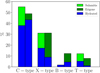 |
Fig. 5 Proportion of asteroids from each primitive class with respect to the total number of primitive asteroids found for each family. The percentage of asteroids showing the 0.7 μm absorption band within each class is shown in blue. We compare the results obtained for the Sulamitis family (this work, light green) with those obtained in Morate et al. (2016) for the Erigone family (dark green). |
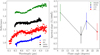 |
Fig. 6 Visible spectra of asteroid (752) Sulamitis currently available (left panel). The four spectra are normalized to unity at 0.55 μm and offset vertically for clarity. In the right panel we show the computed slope of the spectra as a function of phase angle at the moment of the observations. |
Information for the different spectra of (752) Sulamitis available in the literature, and also for the ones we have obtained.
4 Discussion
No previous spectroscopic studies had been performed until now on the Sulamitis nor the Clarissa primitive collisional families. Only the parent bodies, (752) Sulamitis and (302) Clarissa had been observed before: (752) was observed as part of the SMASS and the S3 OS2 surveys (Xu et al. 1995; Lazzaro et al. 2004) and (302) Clarissa was observed as part of the ECAS survey (Zellner et al. 1985). (752) Sulamitis shares the particular spectroscopic feature at 0.7 μm with most of its family members (about 60%), while the spectrum of (302) Clarissa does not show this hydration feature, as is the case for the large majority of its family members. The other two primitive low-inclination families located in the inner belt, Polana and Erigone, have been studied recently (Walsh et al. 2013; Dykhuis & Greenberg 2015; de León et al. 2016; Pinilla-Alonso et al. 2016; Morate et al. 2016). In the next paragraphs we discuss the results obtained here for the Sulamitis and Clarissa families, and we will compare those with the ones on the literature for Polana and Erigone.
The Sulamitis family presents a different distribution of taxonomical classes from that of the Clarissa family. In our sample, we found primarily C- and X-type objects (50.0% and 28.1% respectively), few T-types (10.9%), and just one B-type, plus six interlopers (V-, A-, and S-types), in agreement with the classification proposed in Nesvorný et al. (2015), where Sulamitis is classified as a C-type. On the contrary, in the Clarissa family, although there is a similar C-type proportion (48.5%), we found that B-types are more common (33.3%), with few X-types (15.2%) and only one S-type. This result differs from the classification presented in Nesvorný et al. (2015) for the Clarissa family, where it appears as an X-type (using SDSS photometric data), while our results from visible spectroscopy point to a C/B-type family. In addition, the slope distribution for the objects in the Sulamitis family is fairly redder than that of the Clarissa family, as can be seen in Fig. 3, mainly due to the larger fraction of X-types found in the former. These results confirm the primitive composition of both families. However, their surface compositions seem to be different.
When comparing the Sulamitis family slope distribution with the slope distribution obtained in Morate et al. (2016) for the Erigone family, we find that they are very similar (see lower-left panel of Fig. 3), with a mean spectral slope of 2.1 ± 1.8%∕1000 Å for the Sulamitis family, vs. a value of 1.8 ± 2.0%∕1000 Å for the Erigone family. The same happens when we compare the slope distributions of the Clarissa and Polana families and their mean spectral slopes: 0.2 ± 2.0%∕1000 Å for Clarissa vs. − 0.5 ± 1.3%∕1000 Å for Polana (de León et al. 2016). The KS-test we run on both pairs of distributions (Sulamitis vs. Erigone, and Clarissa vs. Polana), tells us that we cannot reject the hypothesis that one sample pair comes from one common distribution, and the other sample pair comes from another common distribution.
In addition, both family pairs (Sulamitis-Erigone and Clarissa-Polana) show a similar presence of the 0.7 μm aqueous alteration feature: Sulamitis and Erigone present, respectively, 60.3% (this work) and 57.7% (Morate et al. 2016)of primitive asteroid spectra with the hydration band (see Fig. 5 for a more in-depth comparison of the aqueous alteration presence between these families); on the other hand, Clarissa and Polana show, respectively, three (this work) and one (de León et al. 2016) spectra with the 0.7 μm absorption feature within the two studied samples, that is, there are two “wet” families (Erigone and Sulamitis), and two “dry” families (Polana and Clarissa).
The presence of a primitive collisional family, Sulamitis, located between 2.4 and 2.5 AU, and with the majority of its members showing the 0.7 μm hydration band, is in good agreement with the results presented by Fornasier et al. (2014), where they suggested that the aqueous alteration processes dominate in primitive asteroids located between 2.3 and 3.1 AU. Moreover, it is stated that the proportion of hydrated primitive objects (regardless the taxonomic class) in the region where the Sulamitis family is located is 64%, in good agreement with the proportion of hydrated objects we have found in our sample, 60.3% (35 out of 58).
As it was the case in Morate et al. (2016), we found no significant correlations between the band depths or the band centers and the taxonomical class, the orbital parameters, or the albedo of the objects. A similar lack of correlation is found by Carvano et al. (2003) and Fornasier et al. (2014) in their respective studies for asteroids through the whole main belt. Interestingly, these and other authors find that the percentage of hydrated asteroids is somehow correlated with their size, the aqueous alteration process being less effective for bodies smaller than 50 km, and dominating in the 50−240 km size range. We cannot search for correlations between hydration and size in our sample, as we are studying asteroids within collisional families having about the same size: the mean sizes of the objects studied in this work in the Sulamitis and the Erigone collisional families are 5.5 km and 4.2 km respectively. The presence of such large fraction of small asteroids showing the 0.7 μm absorption band can be explained by the fact that they are fragments of larger bodies that were aqueously altered: both (752) Sulamitis and (163) Erigone have diameters larger than 50 km and therefore the parent bodies of these two families were large enough to retain water ice in their interiors and produce internal heating sufficient to melt the ice.
Regarding the difference in the presence of the aqueous alteration for both families, it is most likely explained by their two parent bodies. Asteroid (302) Clarissa shows no signs at all of the hydration feature at 0.7 μm, while (752) Sulamitis shows evidence of aqueous alteration. Therefore, the presence of the hydration feature in the spectra of most of its family members is somewhat expected for the latter. This was also the case for asteroid (163) Erigone and the members of its collisional family (Morate et al. 2016). In this paper we proposed that space weathering could be acting on the surfaces of C-type asteroids by removing the aqueous alteration band: the older the family, the less the fraction of objects showing the 0.7 μm absorption feature. According to Bottke et al. (2015), the estimated ages for Clarissa, Erigone, Sulamitis, and Polana families are ~60 Myr, 130 ± 30 Myr, 200 ± 40 Myr, and 1400 ± 150 Myr, respectively. Therefore, we can rule out the space weathering explanation, since, according to these ages, Clarissa, the youngest member of this group, should present a higher number of hydrated asteroids if this hydration feature was present at any point during the family’s life.
To end the discussion, we would like to note that Sulamitis and Clarissa are two primitive families which share with the Erigone and Polana families, respectively, a) similar proportion of taxonomic classes; b) similar slope distribution; c) similar presence of the 0.7 μm aqueous alteration feature; and d) similar proper orbital elements, specifically semi-major axis and inclination (see Fig. 1 from Morate et al. 2016). Having this in mind, we would like to propose here the possibility of a link between these four families (two links, actually). One link between Erigone and Sulamitis (which, in addition, have similar ages), and another link between the Clarissa and Polana families. The question of whether they could be related in some way, for example cratering events or fragmentation of bigger asteroids Milani et al. (2014), is open for future discussion.
5 Conclusions
We studied a total of 97 visible spectra of asteroids in the Sulamitis and Clarissa primitive families. All spectra were obtained with the 10.4 m Gran Telescopio Canarias and had never been spectroscopically observed before (with the exception of the parent bodies). (752) Sulamitis was also observed with the 2.5 m Isaac Newton Telescope. We have sampled 64 out of the total of 303 asteroids in the Sulamitis family (~ 21% of the family) and 33 out of 179 in the case of Clarissa (~18%).
In terms of taxonomical distribution, in the case of the Sulamitis family we found that 50% of the asteroids are classified as C-type objects, 28% as X-types, 11% as T-types, and just one B-type, being the 9% of the objects in the sample spectral interlopers (three V-types, two A-types, and one Sr-type). The taxonomical distribution for the Clarissa family is clearly different from that ofSulamitis: we see a similar proportion of C-types (48%), but 33% of the objects are classified as B-types, 15% as X-types, and we found just one interloper.
The study of aqueous alteration performed on the Sulamitis primitive sample shows a high number of hydrated asteroids: 35 out of 58 (about60%). This percentage of aqueously altered asteroids is comparable with the results obtained by Morate et al. (2016) for the Erigone collisional family (about 58%). Moreover, the taxonomical distribution is very similar between Sulamitis and Erigone families. The Clarissa family, however, does not show almost any signs of hydration (just three objects in the sample present the aqueous alteration band). This result, together with its taxonomical and slope distribution is, again, comparable with the results obtained by de León et al. (2016) for the Polana family.
Given all the physical similarities found between these families, and given that they also share similar orbital properties, we hereby propose the possibility of the existence of a link between the Erigone and Sulamitis families, and also between the Polana and the Clarissa family. Future work should include a more detailed analysis on the dynamical evolution of these groups, in order to confirm or discard a possible common origin.
Acknowledgements
D.M. gratefully acknowledges the Spanish Ministry of Economy and Competitiveness (MINECO) for the financial support received in the form of a Severo-Ochoa PhD fellowship, within the Severo-Ochoa International PhD Program. D.M., J.d.L.and J.L. acknowledge support from the project AYA2012-39115-C03-03 and ESP2013-47816-C4-2-P (MINECO). J.d.L. acknowledges financial support from the Spanish MINECO under the 2015 Severo Ochoa Program MINECO SEV-2015-0548. M.D.P. acknowledges support from the CAPES (Brazil). H.C. acknowledges support from NASA’s Near-Earth Object Observations program and from the Center for Lunar and Asteroid Surface Science funded by NASA’s SSERVI program at the University of Central Florida. D.M. gratefully acknowledges Dr. Jorge Carvano for the discussions on the improvement of the detection method for the aqueous alteration features. The results obtained in this paper are based on observations made with the Gran Telescopio Canarias (GTC), installed in the Spanish Observatorio del Roque de los Muchachos of the Instituto de Astrofísica de Canarias, in the island of La Palma. The authors thank Marcel Popescu for the observing time to obtain the second spectrum of (752) on program C97-2015 on the Isaac Newton Telescope (INT).
Appendix A: Visible spectra
We present here the visible spectra of the asteroids from the Sulamitis and Clarissa collisional families studied in this paper. A total of 64 and 33 asteroids were observed from each family, respectively. Spectra are normalized to unity at 0.55 μm.
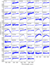 |
Fig. A.1 Visible spectra of the 64 observed asteroids from the Sulamitis family. |
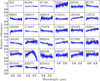 |
Fig. A.2 Visible spectra of the 33 observed asteroids from the Clarissa family. |
Appendix B: Additional tables
Observational circumstances for the asteroids presented in this work.
Orbital and physical parameters of the observed asteroids.
References
- Barucci, M. A., Doressoundiram, A., Fulchignoni, M., et al. 1998, Icarus, 132, 388 [NASA ADS] [CrossRef] [Google Scholar]
- Bevington, P. R., & Robinson, D. K. 1992, Data reduction and error analysis for the physical sciences (New York: McGraw-Hill) [Google Scholar]
- Binzel, R. P., & Xu, S. 1993, Science, 260, 186 [NASA ADS] [CrossRef] [Google Scholar]
- Bottke, W. F., Morbidelli, A., Jedicke, R., et al. 2002, Icarus, 156, 399 [NASA ADS] [CrossRef] [Google Scholar]
- Bottke, W. F., Vokrouhlický, D., Walsh, K. J., et al. 2015, Icarus, 247, 191 [NASA ADS] [CrossRef] [Google Scholar]
- Bus, S. J., & Binzel, R. P. 2002, Icarus, 158, 146 [NASA ADS] [CrossRef] [Google Scholar]
- Campins, H., Morbidelli, A., Tsiganis, K., et al. 2010, ApJ, 721, L53 [NASA ADS] [CrossRef] [Google Scholar]
- Campins, H., de León, J., Morbidelli, A., et al. 2013, AJ, 146, 26 [NASA ADS] [CrossRef] [Google Scholar]
- Carvano, J. M., Mothé-Diniz, T., & Lazzaro, D. 2003, Icarus, 161, 356 [NASA ADS] [CrossRef] [Google Scholar]
- Cepa, J. 2010, in Highlights of Spanish Astrophysics V, eds. J. M. Diego, L. J. Goicoechea, J. I. González-Serrano, & J. Gorgas, 15 [NASA ADS] [CrossRef] [Google Scholar]
- Cepa, J., Aguiar, M., Escalera, V. G., et al. 2000, in Optical and IR Telescope Instrumentation and Detectors, eds. M. Iye, & A. F. Moorwood, SPIE Conf. Ser., 4008, 623 [NASA ADS] [CrossRef] [Google Scholar]
- Clark, B. E., Helfenstein, P., Bell, J. F., et al. 2002, Icarus, 155, 189 [NASA ADS] [CrossRef] [Google Scholar]
- Dahlgren, M., Lagerkvist, C.-I., Fitzsimmons, A., Williams, I. P., & Gordon, M. 1997, A&A, 323, 606 [NASA ADS] [Google Scholar]
- de León, J., Pinilla-Alonso, N., Delbo, M., et al. 2016, Icarus, 266, 57 [NASA ADS] [CrossRef] [Google Scholar]
- DeMeo, F. E., Binzel, R. P., Slivan, S. M., & Bus, S. J. 2009, Icarus, 202, 160 [NASA ADS] [CrossRef] [Google Scholar]
- De Prá, M. N., Pinilla-Alonso, N., Carvano, J. M. F., et al. 2017, Icarus, accepted [Google Scholar]
- Dykhuis, M. J., & Greenberg, R. 2015, Icarus, 252, 199 [NASA ADS] [CrossRef] [Google Scholar]
- Fornasier, S., Lazzarin, M., Barbieri, C., & Barucci, M. A. 1999, A&AS, 135, 65 [NASA ADS] [CrossRef] [EDP Sciences] [Google Scholar]
- Fornasier, S., Lantz, C., Barucci, M. A., & Lazzarin, M. 2014, Icarus, 233, 163 [NASA ADS] [CrossRef] [Google Scholar]
- Gayon-Markt, J., Delbo, M., Morbidelli, A., & Marchi, S. 2012, MNRAS, 424, 508 [NASA ADS] [CrossRef] [Google Scholar]
- Gradie, J., & Veverka, J. 1986, Icarus, 66, 455 [NASA ADS] [CrossRef] [Google Scholar]
- Gradie, J., Veverka, J., & Buratti, B. 1980, in Lunar and Planetary Science Conference Proceedings 11, ed. S. A. Bedini,799 [Google Scholar]
- Howell, E. S., Rivkin, A. S., Vilas, F., et al. 2011, EPSC-DPS Joint Meeting 2011, 637 [Google Scholar]
- Landolt, A. U. 1992, AJ, 104, 340 [NASA ADS] [CrossRef] [Google Scholar]
- Lauretta, D. S., Drake, M. J., Benzel, R. P., et al. 2010, Meteoritics and Planetary Science Supplement, 73, 5153 [NASA ADS] [Google Scholar]
- Lazzaro, D., Angeli, C. A., Carvano, J. M., et al. 2004, Icarus, 172, 179 [CrossRef] [Google Scholar]
- Lumme, K., & Bowell, E. 1981, AJ, 86, 1705 [NASA ADS] [CrossRef] [Google Scholar]
- Luu, J. X., & Jewitt, D. C. 1990, AJ, 99, 1985 [NASA ADS] [CrossRef] [Google Scholar]
- Mainzer, A. K., Bauer, J. M., Cutri, R. M., et al. 2016, NEOWISE Diameters and Albedos V1.0. EAR-A-COMPIL-5-NEOWISEDIAM-V1.0. NASA Planetary Data System [Google Scholar]
- Milani, A., Cellino, A., Knezević, Z., et al. 2014, Icarus, 239, 46 [NASA ADS] [CrossRef] [Google Scholar]
- Morate, D., de León, J., De Prá, M., et al. 2016, A&A, 586, A129 [NASA ADS] [CrossRef] [EDP Sciences] [Google Scholar]
- Nesvorny, D. 2015, Nesvorny HCM Asteroid Families V3.0. EAR-A-VARGBDET-5-NESVORNYFAM-V3.0. NASA Planetary Data System [Google Scholar]
- Nesvorný, D., Broz, M., & Carruba, V. 2015, Identification and Dynamical Properties of Asteroid Families, eds. P. Michel, F. E. DeMeo, & W. F. Bottke, 297 [Google Scholar]
- Pinilla-Alonso, N., de León, J., Walsh, K. J., et al. 2016, Icarus, 274, 231 [NASA ADS] [CrossRef] [Google Scholar]
- Popescu, M., Birlan, M., & Nedelcu, D. A. 2012, A&A, 544, A130 [NASA ADS] [CrossRef] [EDP Sciences] [Google Scholar]
- Press, W. H. 1992, Numerical recipes 2nd edn.: The art of scientific computing (Cambridge University Press) [Google Scholar]
- Rivkin, A. S. 2012, Icarus, 221, 744 [NASA ADS] [CrossRef] [Google Scholar]
- Tsuda, Y., Yoshikawa, M., Abe, M., Minamino, H., & Nakazawa, S. 2013, Acta Astronautica, 91, 356 [NASA ADS] [CrossRef] [Google Scholar]
- Vilas, F. 1994, Icarus, 111, 456 [NASA ADS] [CrossRef] [Google Scholar]
- Vilas, F., & Gaffey, M. J. 1989, Science, 246, 790 [NASA ADS] [CrossRef] [PubMed] [Google Scholar]
- Vokrouhlický, D., Broz, M., Bottke, W. F., Nesvorný, D., & Morbidelli, A. 2006, Icarus, 182, 118 [NASA ADS] [CrossRef] [Google Scholar]
- Walsh, K. J., Delbó, M., Bottke, W. F., Vokrouhlický, D., & Lauretta, D. S. 2013, Icarus, 225, 283 [NASA ADS] [CrossRef] [Google Scholar]
- Xu, S., Binzel,R. P., Burbine, T. H., & Bus, S. J. 1995, Icarus, 115, 1 [NASA ADS] [CrossRef] [Google Scholar]
- Zappala, V., & Cellino, A. 1994, in Asteroids, Comets, Meteors 1993, eds. A. Milani, M. di Martino, & A. Cellino, IAU Symp., 160, 395 [NASA ADS] [Google Scholar]
- Zappala, V., Cellino, A., Farinella, P., & Knezevic, Z. 1990, AJ, 100, 2030 [NASA ADS] [CrossRef] [Google Scholar]
- Zellner, B., Tholen, D. J., & Tedesco, E. F. 1985, Icarus, 61, 355 [NASA ADS] [CrossRef] [Google Scholar]
Online tool for modeling of asteroid spectra: http://m4ast.imcce.fr/
All Tables
Right ascension, declination, and visible magnitude for the solar analog stars used to obtain the reflectance spectra of the observed asteroids.
Information for the different spectra of (752) Sulamitis available in the literature, and also for the ones we have obtained.
All Figures
|
Fig. 1 Distribution of the taxonomical classes for the sample of 64 Sulamitis family asteroids (top panel) and the 33 Clarissa family asteroids (bottom panel) studied in this paper. The “Other” class includes all non-primitive taxonomies (S-types, V-types, and A-types). |
| In the text | |
|
Fig. 2 Absolute magnitude (H) of the asteroids from the Sulamitis and Clarissa families as a function of their proper semi-major axes. Both families are shown in gray. The colored circles correspond to the objects observed in this study. Objects depicted in blue are primitive asteroids (C, X, B, T, and subclasses), while objects in red are non-primitive (A-, V-, and S-types). The family parent asteroids, (752) Sulamitis and (302) Clarissa, are represented as stars and are the largest objects in the families. |
| In the text | |
|
Fig. 3 Comparison of the spectral slope distributions of the primitive families in the inner main belt. The bin size is 0.87%/1000 Å. From left to right, top to bottom: sulamitis vs. Clarissa (this work), Polana vs. Erigone (the largest families, see Morate et al. 2016 for in-depth results), Clarissa vs. Polana, and Sulamitis vs. Erigone. Sulamitis and Erigone have been depicted in red, and Clarissa and Polana in blue. The vertical lines represent the mean values of the slope distributions. See text for more details. |
| In the text | |
|
Fig. 4 Cumulative distribution function (CDF) of the slopes for the four primitive families of the inner main belt: Sulamitis and Clarissa (this work), Polana (de León et al. 2016), and Erigone (Morate et al. 2016). The Kolmogorov-Smirnov test compares the CDFs and gives an estimation of the differences. |
| In the text | |
|
Fig. 5 Proportion of asteroids from each primitive class with respect to the total number of primitive asteroids found for each family. The percentage of asteroids showing the 0.7 μm absorption band within each class is shown in blue. We compare the results obtained for the Sulamitis family (this work, light green) with those obtained in Morate et al. (2016) for the Erigone family (dark green). |
| In the text | |
|
Fig. 6 Visible spectra of asteroid (752) Sulamitis currently available (left panel). The four spectra are normalized to unity at 0.55 μm and offset vertically for clarity. In the right panel we show the computed slope of the spectra as a function of phase angle at the moment of the observations. |
| In the text | |
|
Fig. A.1 Visible spectra of the 64 observed asteroids from the Sulamitis family. |
| In the text | |
|
Fig. A.2 Visible spectra of the 33 observed asteroids from the Clarissa family. |
| In the text | |
Current usage metrics show cumulative count of Article Views (full-text article views including HTML views, PDF and ePub downloads, according to the available data) and Abstracts Views on Vision4Press platform.
Data correspond to usage on the plateform after 2015. The current usage metrics is available 48-96 hours after online publication and is updated daily on week days.
Initial download of the metrics may take a while.