| Issue |
A&A
Volume 609, January 2018
|
|
|---|---|---|
| Article Number | A32 | |
| Number of page(s) | 7 | |
| Section | The Sun | |
| DOI | https://doi.org/10.1051/0004-6361/201731697 | |
| Published online | 22 December 2017 | |
Quasi-periodic changes in the 3D solar anisotropy of Galactic cosmic rays for 1965–2014
1 Institute of Math. and Physics, Siedlce University, 3 Maja 54 Street, 08-110 Siedlce, Poland
e-mail: renatam@uph.edu.pl
2 Institute of Geophysics, Tbilisi State University, Tbilisi 380093, Georgia
e-mail: alania@uph.edu.pl
Received: 2 August 2017
Accepted: 14 November 2017
Aims. We study features of the 3D solar anisotropy of Galactic cosmic rays (GCR) for 1965−2014 (almost five solar cycles, cycles 20−24). We analyze the 27-day variations of the 2D GCR anisotropy in the ecliptic plane and the north-south anisotropy normal to the ecliptic plane. We study the dependence of the 27-day variation of the 3D GCR anisotropy on the solar cycle and solar magnetic cycle. We demonstrate that the 27-day variations of the GCR intensity and anisotropy can be used as an important tool to study solar wind, solar activity, and heliosphere.
Methods. We used the components Ar, Aϕ and At of the 3D GCR anisotropy that were found based on hourly data of neutron monitors (NMs) and muon telescopes (MTs) using the harmonic analyses and spectrographic methods. We corrected the 2D diurnal (~24-h) variation of the GCR intensity for the influence of the Earth magnetic field. We derived the north-south component of the GCR anisotropy based on the GG index, which is calculated as the difference in GCR intensities of the Nagoya multidirectional MTs.
Results. We show that the behavior of the 27-day variation of the 3D anisotropy verifies a stable long-lived active heliolongitude on the Sun. This illustrates the usefulness of the 27-day variation of the GCR anisotropy as a unique proxy to study solar wind, solar activity, and heliosphere. We distinguish a tendency of the 22-yr changes in amplitude of the 27-day variation of the 2D anisotropy that is connected with the solar magnetic cycle. We demonstrate that the amplitudes of the 27-day variation of the north-south component of the anisotropy vary with the 11-yr solar cycle, but a dependence of the solar magnetic polarity can hardly be recognized. We show that the 27-day recurrences of the GG index and the At component are highly positively correlated, and both are highly correlated with the By component of the heliospheric magnetic field.
Key words: Sun: activity / Sun: heliosphere / solar wind / Sun: rotation
© ESO, 2017
1. Introduction
The flux of the Galactic cosmic rays (GCRs) measured at Earth consists of an isotropic and an anisotropic part. The isotropic part contains the various quasi-periodic changes with different timescales (from hours to several years), see, for instance, Kudela & Sabbah (2016), Chowdhury et al. (2016), Bazilevskaya et al. (2014, and references therein), and 3D spatial density gradients (Kozai et al. 2014). The anisotropic part is generally reflected in the solar diurnal variation (~24-h wave), assuming that while Earth completes one rotation, the location of a source of the anisotropic stream remains unchanged. The mechanism of the solar diurnal anisotropy was explained by Ahluwalia & Dessler (1962) and also by Krymsky (1964) and Parker (1964), independently of each other, based on the anisotropic diffusion-convection theory of GCR propagation in the heliosphere. Chen & Bieber (1993) have shed light on this problem assuming that the 3D GCR anisotropy is a combination of the 2D solar ecliptic and the north-south anisotropies. The 2D solar ecliptic anisotropy causes the daily variation in the count rate of ground-based detectors (e.g., neutron monitors (NMs) or muon telescopes (MTs)) that rotate with Earth; the north-south anisotropy reveals a flow of GCRs normal to the ecliptic plane. Swinson (1969) proposed that the north-south anisotropy might have occurred as a result of the drift that is caused by positive heliocentric radial density gradient Gr of cosmic rays and the By component of the heliospheric magnetic field (HMF; expressed as the vector product, By × Gr).
Of recent publications devoted to the GCR anisotropy, we mention, for example, Kudela & Sabbah (2016), Ahluwalia et al. 2015, Munakata et al. (2014), Sabbah (2013), and Oh et al. 2010. However, quasi-periodic changes of the GCR anisotropy connected with the solar rotation (called the 27-day variation here) were studied rarely until Alania et al. (2005, 2008) examined the ecliptic plane anisotropy (2D case) and the north-south component alone for polar-located NMs was considered by Owens et al. (1980). Swinson and coauthors (Swinson & Yasue 1991; 1992; Swinson et al. 1993; Swinson & Fuji 1995) reported the significant correlation between the 27-day variation of the north-south anisotropy for MT data and the tilt angle of the heliospheric neutral sheet. Alania et al. (2005, 2008) and Gil et al. (2012) analyzed the periods near the minima epochs of solar activity. They demonstrated that the amplitude of the 27-day variation of the 2D anisotropy is smaller in the negative-polarity period than in the positive-polarity period of the HMF.
The main aim of this paper is twofold: (1) to investigate the 27-day variation of the 3D GCR solar anisotropy and its long-term changes during about five solar cycles, cycles 20−24; and (2) to study the time lines of the 27-day variations of the north-south component of the GCR anisotropy and the 2D GCR anisotropy in the ecliptic plane.
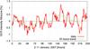 |
Fig. 1 Hourly data of Moscow NM in January 2−11, 2007 (red line) with the 25 h trend (green line). |
2. Data and methods
We used data of the neutron monitors located at Kiel, Moscow, Oulu, Deep River, and Climax, which have magnetic cutoff rigidities of Rc< 5 GV to clearly reveal the 3D GCR anisotropy. The pressure-corrected hourly data of the GCR intensity were normalized as ![\hbox{$I[\%]=\frac{x_{i}-\overline{x}}{\overline{x}}$}](/articles/aa/full_html/2018/01/aa31697-17/aa31697-17-eq13.png) , where
, where  is average count rate of the observed GCR intensity. We excluded trends larger than the diurnal variation (24 h) using the 25-h moving-average method. As an example, we present the hourly data of the Moscow NM for January 2−11, 2007, in Fig. 1, and the same “detrended” data in Fig. 2. Figures 1 and 2 demonstrate that the GCR intensity (Fig. 1) alternates under the influence of a trend with a period longer than 25 h, while the “detrended” data (Fig. 2) show an intensity fluctuation of about zero, which is essential for a harmonic analysis.
We calculated the daily radial ar and tangential aϕ components of the diurnal variation of the GCR intensity by normalized and detrended hourly data of the GCR intensity using the harmonic analyses method (e.g., Gubbins 2004): 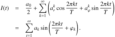 (1)Here,
 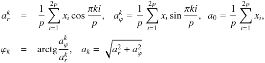 2p = 24 h, and xi designates the hourly data of the GCR intensity for each NM. We corrected the daily radial ar and tangential aϕ components of the diurnal variation of the GCR intensity for the influence of the terrestrial magnetic field (Rao et al. 1963; Dorman et al. 1972; Dorman 2009), taking into account the asymptotic acceptance cone that is characteristic for each NM. This was done by rotating the corresponding angle λ (asymptotic longitude) for each NM. We calculated the radial
  and the tangential
  components of the diurnal variation of the GCR intensity corrected for the influence of the terrestrial magnetic field using the expressions
  (2)Furthermore, we excluded from consideration the amplitudes >0.7% as an anomalous event related to the disturbances in interplanetary space, generally corresponding to the periods of Forbush decreases. Fewer than 2−3% of the total number of days were excluded.
The amplitude of the diurnal variation of the GCR intensity  at any point of the observation (by a NM) with the geomagnetic cutoff rigidity Rc and the average atmospheric depth hj can be defined as
 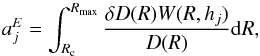 (3)where
  is the rigidity spectrum of the diurnal variation of the GCR intensity, and
  is the coupling function (Dorman 1963; Yasue et al. 1982); Rmax is the upper limit of the rigidity beyond which the amplitudes of the diurnal variation of the GCR intensity vanish. For the power type of the rigidity spectrum
  , we can write
  (4)where is the observed amplitude of the diurnal variation of the GCR intensity for jth NM, and Aj is the corresponding amplitude of the anisotropy of GCRs in the heliosphere.
Details of the neutron monitors and values of corresponding coupling coefficients (CC) vs. solar activity.
The values of Aj must be the same in the scope of the calculation accuracy for arbitrary NM data when the parameter pairs γ and Rmax are properly determined. The similarity of the Aj values we found for the different NMs is a decisive factor that confirms that the data of the given NM are reliable. We converted the radial ar and azimuthal aϕ components of the diurnal GCR variation into the radial Ar and azimuthal Aϕ components of the GCR anisotropy in the heliosphere (free space; Dorman 1963; Yasue et al. 1982), 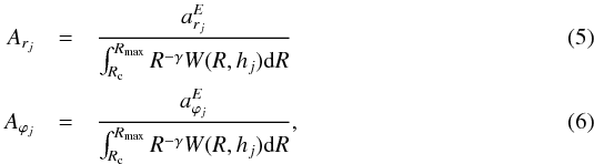 where the expression
  is called the coupling coefficient (CC). This is the ratio of the observed amplitude of the diurnal variation to the corresponding amplitude of the anisotropy of cosmic rays in the heliosphere. We provide a conversion for the same set of parameters as in Bieber & Chen (1991), namely Rmax = 100 GV and spectral index γ=0. This selection of the parameters Rmax and γ is reasonable because the criterion of equality of the Aj values (the amplitudes of the GCR anisotropy in the heliosphere) found for the different NMs is satisfied. We found that for γ = 0.5, there are no great changes in the results, meaning that the rigidity dependence of the anisotropy is reasonably weak for the energy range of GCR particles to which the NMs respond; a hard GCR anisotropy spectrum was found in Hall et al. (1996).
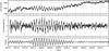 |
Fig. 3 Temporal changes of the daily GCR intensity for Oulu NM for the period of 2007−2009 (top) and corresponding to this period the same data detrended over 29 days (middle) and filtered periodic oscillation with the band-pass period within 24−32 days (bottom). |
The details of the NMs we used and the corresponding CC values versus solar activity are presented in Table 1.
We also used results of the 3D GCR anisotropy calculated by the group of Institute of Terrestrial Magnetism, Ionosphere and Radio Wave Propagation of the Russian Academy of Sciences (IZMIRAN; Abunina et al. 2015; Belov et al. 2005) by applying the global spectrographic method (GSM; Krymsky et al. 1966; 1967) which contains all operating NMs. Furthermore, to study the features of the 3D GCR anisotropy in the relatively wide range of the GCR spectrum, we used data from the Nagoya MTs (Munakata et al. 2014) with a median rigidity of ~60 GV.
We used the power spectrum density (PSD) method to reveal the quasi-periodicity in the analyzed time series; this method decomposes the time series into frequency (ω ) and period (T) components (e.g., Otnes & Enochson 1972; Press et al. 2002),  (7)where R(t) is the autocorrelation function. In a discrete case, we have
  (8)here
  is the autocorrelation function of the time series xi and W is the window function (we used Parzen’s window function). The PSD of each frequency ω is calculated as | ψ2(ω) | Hz-1.
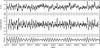 |
Fig. 4 Same as in Fig. 3 but for Ar component of the GCR anisotropy for Oulu NM. |
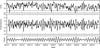 |
Fig. 5 Same as in Fig. 3 but for Aϕ component of the GCR anisotropy for Oulu NM. |
3. 27-day variation of the 2D GCR anisotropy in the ecliptic plane
Unfortunately, a complete precise method for a simultaneous calculation of the radial Ar, azimuthal Aϕ and latitudinal (north-south) At components of the 3D GCR anisotropy based on the worldwide network of NMs and MTs is currently not available. The Ar and Aϕ components can be calculated using the GSM and harmonic analyses methods, which are based on data of the NMs with cutoff rigidities <5 GV; in addition, a latitudinal At (north-south) component can be calculated within the scope of the arbitrary constant, but only with the GSM method. Additionally, the At component can be estimated as the difference of two NMs that are located in the regions of the north and south poles (Chen & Bieber 1993), and At can also be estimated by directed MTs. However, these data are not homogenous, and to study features of 3D anisotropy (e.g., the 27-day variation of the 3D anisotropy), we have to use results for Ar, Aϕ and At that are obtained in different ways.
The 27-day variations of the GCR intensity (e.g., Richardson et al. 1999; Dunzlaff et al. 2008; Guo & Florinsky 2014; 2016; Kopp et al. 2017; Gil & Mursula 2017) and the anisotropy (e.g., Modzelewska & Alania 2012; Mavromichalaki et al. 2016) have a sporadic character. Their amplitudes significantly increase and decrease on average during four to six solar rotation periods. However, they are not completely random phenomena. Generally, some levels of the 27-day variation amplitudes of the GCR intensity and anisotropy always exist that are above the background fluctuations. This statement is demonstrated in Figs. 3−5, where we present the changes in GCR intensity (Fig. 3), and we also show the Ar (Fig. 4) and Aϕ (Fig. 5) components of the GCR anisotropy for the period of 2007−2009 for the Oulu NM. We present in Figs. 3−5 the corresponding data “detrended” by moving smoothing intervals of 29 days and a filtered periodic oscillation with the bandpass period within 24−32 days. Figures 3−5 show periods with a well-pronounced 27-day recurrence with high amplitudes of the 27-day GCR intensity variations and the anisotropy components, as well as very small amplitudes in other periods. This behavior of the 27-day variations of the GCR intensity and solar anisotropy is related with some disparate mechanisms. The 27-day variation of the GCR intensity is mainly connected with heliolongitudinal asymmetry of the solar wind and the solar activity and their dependences on heliolatitudes. This means that the 27-day variation in GCR intensity contributes a fairly large part of interplanetary space. At the same time, the convection-diffusion mechanism of the solar anisotropy (Krymsky 1964; Parker 1964) is determined by local processes near the Earth orbit and requires a smaller part of the heliosphere. Above all, especially in the solar activity minima epochs, the 27-day variation in anisotropy is rarely observed, which is apparently connected with the drift of cosmic rays in the sector structure of the HMF, while a weak 27-day variation in GCR intensity is observed. The circumstances can be reversed when a clear 27-day GCR intensity variation is observed that does not follow the 27-day anisotropy variation at all. Unfortunately, this phenomenon is currently not fully explained, which indicates that the problem of the 27-day anisotropy and intensity variations is not fully understood so far. No universal mechanism of the 27-day GCR anisotropy and intensity variations is currently available that would account for dynamical changes in features in solar atmosphere and heliosphere sources. Therefore we need to find new properties of the 27-day GCR anisotropy and intensity. This problem is one of the important aims of this paper.
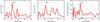 |
Fig. 6 Spectral analysis of the daily radial Ar (left panel), azimuthal Aϕ (middle panel) and phase (right panel) of the 2D GCR anisotropy for Oulu NM for 1971−2014, for all the highest peak is for the period of 25.6 days with 95% confidence level. |
Taking the sporadic nature of the 27-day GCR anisotropy variation into account (it lasts on average foraboutfourtosix solar rotations), studying its behavior for the long period of 1971−2014 is naturally interesting. For this purpose, we applied the spectral analysis method based on the Oulu NM data. The calculation results are presented in Fig. 6. Figure 6 presents the spectral analysis of the daily radial Ar, the azimuthal Aϕ components, and of the phase = arctan(Aϕ/Ar) of the 2D GCR anisotropy for the Oulu NM for the long period of 1971−2014. Figure 6 shows that the Ar and Aϕ components and phase apparently demonstrate quasi-periodic changes related to the Sun’s rotation. For the components Ar and Aϕ and for the phase, the highest peaks correspond to a period of 25.6 days with a confidence level of 95%. Figure 6 shows stable long-lived active heliolongitudes on the Sun that we consider as the source of the 27-day GCR anisotropy variation.
4. 27-day variation of the north-south anisotropy
To study the 27-day variation of the north-south anisotropy, we used two types of data: (1) the daily At component calculated with the GSM for NMs data1, and (2) the daily GG index obtained for MTs2. The GG index (Mori & Nagashima 1979) is the difference between the intensities that are recorded in the geographically north (N2) south (S2) and east (E2)-viewing directional channels for 49 degrees inclination, corresponding to a median rigidity of ~60 GV and calculated as follows: GG = (N2−S2) + (N2−E2).
This method for studying the north-south asymmetry has the advantage that it uses the GCR intensity data from a single location instead of comparing GCR intensities from north and south polar NMs. The GG index as introduced according to Mori & Nagashima (1979) is expected to be free of noise in isotropic intensity caused by Forbush decreases, periodic variations, atmospheric temperature effects, and geomagnetic cutoffs. Although the counting rate of GCR intensities in different directions (N2,S2,andE2) cannot contain exactly the same type of information, the GG is accepted as a good alternative index by the worldwide cosmic ray community (e.g., Munakata et al. 2014). Recently, we analyzed (Modzelewska & Alania 2015) the behavior of the quasi-periodic changes of the GG index for 2007−2012 with the wavelet time-frequency method. In this paper we extend this study of the GG index and the At anisotropy component for 1971−2014 with the PSD method.
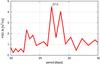 |
Fig. 7 Spectral analysis of the At component of the 3D GCR anisotropy for 1970−2006, the highest peak is for the period of 27 days with 95% confidence level. |
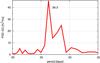 |
Fig. 8 Spectral analysis of the daily GG index for 1971−2014, the highest peak is for the period of 26.3 days with 95% confidence level. |
We present the results of analysis in Figs. 7 and 8. Figure 7 shows the results of the spectral analysis of the At component of the 3D GCR anisotropy for 1971−2006 (data of At are available at the IZMIRAN website until 2006) and Fig. 8 of the GG index for 1971−2014. Figures 7 and 8 show that the At component and the GG index both apparently demonstrate quasi-periodic changes that are related to the Sun’s rotation. For the At component, the period is 27 days and for the GG index, it is 26.3 days with a confidence level of 95%. In Figs. 6 (left panel), 7, and 8, peaks at ~28−29 days are visible, but they are statistically insignificant. We do not exclude the presence of an additional source with an average period of 28−29 days, however, that is due to the differential rotation of the Sun, which manifests itself as the asymmetry of heliolongitudes versus heliolatitudes.
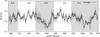 |
Fig. 9 Temporal changes of the average A27A smoothed over 13 solar rotations for all considered NMs (Moscow, Kiel, Oulu, Deep River, Climax) for 1965−2014 during A> 0 and A < 0 polarity epochs; error bars are calculated as standard deviations for considered NMs. |
5. Long-period changes of the 27-day variation amplitudes
5.1. 2D ecliptic plane anisotropy
To study the long-period changes of the 27-day variation amplitudes of the 2D ecliptic plane GCR anisotropy, we calculated the 2D 27-day variation amplitudes of the anisotropy (A27A) for the Climax, Deep River, Kiel, Moscow, and Oulu NM data for 1965−2014. We used the formula (Alania et al. 2005) that combines the 27-day recurrence of the radial and azimuthal components:  (9)Here Arr(27) and Arϕ(27) are the coefficients of the 27-day variation of the Ar component, and Aϕr(27) and Aϕϕ(27) are the coefficients of the 27-day variation of the Aϕ component.
We present the calculation results in Fig. 9. Figure 9 shows the temporal changes in the average amplitude of the 27-day variation of the 2D GCR anisotropy in the ecliptic plane smoothed over 13 solar rotations for the Climax, Deep River, Kiel, Moscow, and Oulu NMs in the time interval 1965−2014; the error bars are calculated as standard deviations for the NMs. The smoothing over 13 solar rotations reduces the error bars, but at the same time, we lost information about the quasi-periodic changes for a time interval of slightly less than one year.
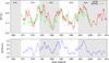 |
Fig. 10 Temporal changes of the amplitudes of the 27-day variation of the GG index (A27GG) and At component (A27At) of the 3D anisotropy (top) and By component of the HMF (A27By) (bottom) smoothed over 13 Sun’s rotations during A> 0 and A< 0 polarity epochs. Values A27GG and A27By are presented for 1971−2014, but A27At – for 1970−2006, data of At is available at the IZMIRAN website up to 2006. |
Figure 9 shows that the average amplitude of the 27-day variation of the GCR 2D anisotropy is larger in the minimum periods of the positive-polarity (A > 0) epochs than in the negative (A < 0) epochs, which agrees well with Alania et al. (2005, 2008). In addition, the time line of the amplitudes of the 27-day variation of the 2D GCR anisotropy shows a tendency of the 22-yr periodicity and a weak but systematic decrease near the periods of solar minimum for an A > 0 polarity (~1975 and ~1996) as well, indicating a weak 11-yr solar cycle modulation. The ecliptic 2D anisotropy components strongly reflect the drift pattern of the cosmic ray flow, and the polarity dependence is consequently apparent in the 27-day variation of the 2D GCR anisotropy.
To reveal a polarity dependence of the 27-day variation of the 2D GCR anisotropy, we calculated the differences in amplitudes between the A > 0 and A < 0 polarities, which is equal to ~40% of the mean value. In particular, the average amplitude of the 27-day variation of the 2D GCR anisotropy A27A for the whole period 1965−2014 is (0.23 ± 0.04)%, and the values of A27A for the consecutive minima are for A > 0 1975–1977 A27A = (0.26 ± 0.01)%, for A < 0 1985–1987 A27A = (0.16 ± 0.01)%, for A > 0 1995–1997 A27A = (0.24 ± 0.02)%,and for A < 0 2007–2009 A27A = (0.18 ± 0.02)%.
5.2. Long-period changes of the 27-day variation amplitudes of the north-south anisotropy
Recently, we showed (Modzelewska & Alania 2015) that the daily GG index is inversely related with the daily By component of the HMF for 2007−2012. This effect, according to Swinson’s (1969) formulation of the north-south anisotropy, is caused by drift, which we consider an acceptable explanation. To study the nature of the north-south asymmetry, we calculated the 27-day variation amplitudes of the GG index (A27GG), At (A27At) and By components (A27By) with the harmonic analysis method for 1971−2014. We present the results in Fig. 10. Figure 10 shows the temporal changes of A27GG and A27At (top), and A27By (bottom) for 1970−2014. The behavior of the amplitudes of the 27-day variations of the GG index and At component is similar and highly positively correlated with the 27-day variation of the By component; all are alternating according to the 11-yr solar cycle. In contrast to the GCR anisotropy in the ecliptic plane, the north-south component has no clear magnetic polarity dependence (e.g., Munakata et al. 2014), so its 27-day recurrence is not expected to be dependent on the magnetic polarity either, which we observe in experimental data.
6. Conclusions
We studied the long-term changes of the 27-day variation amplitudes of the 3D GCR anisotropy for 1965−2014. We showed that the behavior of the 27-variation of the 3D anisotropy verifies the existence of a stable long-lived active heliolongitude on the Sun. This shows that the GCR anisotropy variation is useful as a unique proxy to study the solar wind, solar activity, and the heliosphere. We recovered a tendency of the 22-yr changes of the 27-day variation amplitudes of the 2D anisotropy to be connected with the solar magnetic cycle and a weak 11-yr solar cycle modulation. We demonstrated that the 27-day variation amplitudes of the north-south component of the anisotropy vary in accordance with 11-yr solar cycle, while it is hardly possible to show any dependence on the global solar magnetic field polarity. The 27-day recurrences of the GG index and At component are highly positively correlated, and both are highly correlated with the By component of the HMF. The observed properties of the radial Ar, azimuthal Aϕ, and normal At components and of the GG index demonstrate that quasi-periodic behaviors of the ecliptic 2D and north-south components of the 3D GCR anisotropy are governed by different mechanisms in the ecliptic plane and in the north-south direction. Owing to the complexity of the problem, we are unable to fully explain the physical mechanism of the 27-day anisotropies in 3D space. We are unable to completely clarify the processes related to the 27-day variations of the 3D anisotropy with indipendent theories or experimental data of NMs and MTs. For this purpose, theoretical modeling based on Parker’s transport equation and experimental data have to be considered together.
Acknowledgments
We thank the providers of the data we used in this study, especially the OMNI database, the IZMIRAN group, and the PIs of the Oulu, Moscow, Kiel, Deep River, and Climax NMs and of the Nagoya MTs. R. Aslamazishvili, a member of M. Alania’s scientific group in Tbilisi, participated in calculating the 2D ecliptic anisotropy components of GCRs within the asymptotic acceptance cone in Earth’s magnetic field. The remarks and suggestions of the referee helped us to improve the paper.
References
- Abunina, M., Abunin, A., Belov, A., et al. 2015, J. Phys.: Conf. Ser. 632, 012044 [Google Scholar]
- Ahluwalia, H. S., & Dessler, A. J. 1962, Planet. Space Sci., 9, 195 [NASA ADS] [CrossRef] [Google Scholar]
- Ahluwalia, H. S., Ygbuhay, R. C., Modzelewska, R., et al. 2015, J. Geophys. Res., 120, 8229 [CrossRef] [Google Scholar]
- Alania, M. V., Gil, A., Iskra, K., et al. 2005, in Proc. 29th ICRC, SH3.4, 215 [Google Scholar]
- Alania, M. V., Gil, A., & Modzelewska, R. 2008, Adv. Space Res., 41, 280 [NASA ADS] [CrossRef] [Google Scholar]
- Bazilevskaya, G., Broomhall, A.M., Elsworth, Y., & Nakariakov, V. M. 2014, Space Sci. Rev., 186, 359 [NASA ADS] [CrossRef] [Google Scholar]
- Belov, A. V., Baisultanova, L., Eroshenko, E. A., et al. 2005, J. Geophys. Res., 110, A09S20 [CrossRef] [Google Scholar]
- Bieber, J. W., & Chen, J. 1991, ApJ, 372, 301 [NASA ADS] [CrossRef] [Google Scholar]
- Chen, J., & Bieber, J. W. 1993, ApJ, 405, 375 [NASA ADS] [CrossRef] [Google Scholar]
- Chowdhury, P., Kudela, K., & Moon, Y. J. 2016, Solar Phys., 291, 581 [NASA ADS] [CrossRef] [Google Scholar]
- Dorman, L. I. 1963, Variations of cosmic rays and space exploration (AN SSSR, Moscow) [Google Scholar]
- Dorman, L. I. 2009, Cosmic Rays in Magnetospheres of the Earth and other Planets, Astrophys. Space Sci. Lib., 358 (The Netherlands: Springer) [Google Scholar]
- Dorman, L. I., Gushchina, R. T., Smart, D. F., & Shea, M. A. 1972, Effective Cut-Off Rigidities of Cosmic Rays (Moscow: Nauka) [Google Scholar]
- Dunzlaff, P., Heber, B., Kopp, A., et al. 2008, Ann. Geophys., 26, 3127 [NASA ADS] [CrossRef] [Google Scholar]
- Gil, A., & Mursula, K. 2017, A&A, 599, A112 [NASA ADS] [CrossRef] [EDP Sciences] [Google Scholar]
- Gil, A., Modzelewska, R., & Alania, M. V. 2012, Adv. Space Res., 50, 712 [NASA ADS] [CrossRef] [Google Scholar]
- Gubbins, D. 2004, Time Series Analysis and Inverse Theory for Geophysicists (Cambridge: Cambridge University Press), 21 [Google Scholar]
- Guo, X., & Florinski, V. 2014, J. Geophys. Res.: Space Phys., 119, 2411 [NASA ADS] [CrossRef] [Google Scholar]
- Guo, X., & Florinski, V. 2016, ApJ, 826, 65 [NASA ADS] [CrossRef] [Google Scholar]
- Hall, D. L., Duldig, M. L., & Humble, J. E. 1996, Space Sci. Rev., 78, 401 [NASA ADS] [CrossRef] [Google Scholar]
- Kopp, A., Wiengarten, T., Fichtner, H., et al. 2017, ApJ, 837, 37 [NASA ADS] [CrossRef] [Google Scholar]
- Munakata, K., Kato, Ch., Kuwabara, T., et al. 2014, Earth, Planets and Space, 66, 151 [NASA ADS] [CrossRef] [Google Scholar]
- Krymsky, G. F. 1964, Geomagnetism & Aeronomy, 4, 763 [NASA ADS] [Google Scholar]
- Krymski, G. F., Kuzmin, A. I., Chirkov, N. P., et al. 1966, Geomagnetism & Aeronomy, 6, 991 [Google Scholar]
- Krymski, G. F., Kuzmin, A. I., Chirkov, N. P., et al. 1967, Geomagnetism & Aeronomy, 7, 11 [NASA ADS] [Google Scholar]
- Kudela, K., & Sabbah, I. 2016, Sci. Ch. Technol. Sci., 59, 547 [CrossRef] [Google Scholar]
- Mavromichalaki, H., Papageorgiou, Ch., & Gerontidou, M. 2016, Astrophys. Space Sci., 361, 69 [NASA ADS] [CrossRef] [Google Scholar]
- Modzelewska, R., & Alania, M. V. 2012, Adv. Space Res., 50, 716 [NASA ADS] [CrossRef] [Google Scholar]
- Modzelewska, R., & Alania, M. V. 2015, J. Phys.: Conf. Ser., 632, 012072, 1742 [CrossRef] [Google Scholar]
- Mori, S., & Nagashima, K. 1979, Planet. Space Sci., 27, 39 [NASA ADS] [CrossRef] [Google Scholar]
- Munakata, K., Kozai, M., Kato, C., & Kota, J. 2014, ApJ, 791, 22 [NASA ADS] [CrossRef] [Google Scholar]
- Oh, S. Y., Yi, Y., & Bieber, J. W. 2010, Sol. Phys., 262, 199 [NASA ADS] [CrossRef] [Google Scholar]
- Otnes, R. K., Enochson, L. 1972, Digital Time Series Analysis (New York: John Wiley and Sons), 191 [Google Scholar]
- Owens, A. J., Duggal, S. P., Pomerantz, M. A., & Tolba, M. F. 1980, ApJ, 236, 1012 [NASA ADS] [CrossRef] [Google Scholar]
- Parker, E. N. 1964, Planet. Space Sci., 12, 735 [NASA ADS] [CrossRef] [Google Scholar]
- Press, W. H., Teukolsky, S. A., Vetterling, W. T., & Flannery, B. P. 2002, The Art of Scientific Computing (Cambridge University Press), 550 [Google Scholar]
- Rao, U. R., McCracken, K. G., & Venkatesan, D. 1963, J. Geophys. Res., 68, 345 [NASA ADS] [CrossRef] [Google Scholar]
- Richardson, I. G., Cane, H. V., & Wibberenz, G. 1999, J. Geophys. Res., 104, 12549 [NASA ADS] [CrossRef] [Google Scholar]
- Sabbah, I. 2013, J. Geophys. Res., 118, 4739 [CrossRef] [Google Scholar]
- Swinson, D. B. 1969, J. Geophys. Res., 74, 5591 [NASA ADS] [CrossRef] [Google Scholar]
- Swinson, D. B., & Yasue, S. I. 1991, in Proc. 22nd ICRC, SH, 481 [Google Scholar]
- Swinson, D. B., & Yasue, S. I. 1992, J. Geophys. Res., 92, A12, 19 149 [Google Scholar]
- Swinson, D. B., Yasue, S., & Fujii, Z. 1993, in Proc. 23rd ICRC, 671 [Google Scholar]
- Swinson, D. B., & Fujii, Z. 1995, in Proc. 24th ICRC, SH, 576 [Google Scholar]
- Yasue, S., Sakakibara, S., & Nagashima, K. 1982, Coupling coefficients of cosmic rays daily variations for neutron monitors (Nagoya Report), 7 [Google Scholar]
All Tables
Details of the neutron monitors and values of corresponding coupling coefficients (CC) vs. solar activity.
All Figures
|
Fig. 1 Hourly data of Moscow NM in January 2−11, 2007 (red line) with the 25 h trend (green line). |
| In the text | |
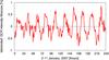 |
Fig. 2 Same data as in Fig. 1 “detrended” with the 25 h. |
| In the text | |
|
Fig. 3 Temporal changes of the daily GCR intensity for Oulu NM for the period of 2007−2009 (top) and corresponding to this period the same data detrended over 29 days (middle) and filtered periodic oscillation with the band-pass period within 24−32 days (bottom). |
| In the text | |
|
Fig. 4 Same as in Fig. 3 but for Ar component of the GCR anisotropy for Oulu NM. |
| In the text | |
|
Fig. 5 Same as in Fig. 3 but for Aϕ component of the GCR anisotropy for Oulu NM. |
| In the text | |
|
Fig. 6 Spectral analysis of the daily radial Ar (left panel), azimuthal Aϕ (middle panel) and phase (right panel) of the 2D GCR anisotropy for Oulu NM for 1971−2014, for all the highest peak is for the period of 25.6 days with 95% confidence level. |
| In the text | |
|
Fig. 7 Spectral analysis of the At component of the 3D GCR anisotropy for 1970−2006, the highest peak is for the period of 27 days with 95% confidence level. |
| In the text | |
|
Fig. 8 Spectral analysis of the daily GG index for 1971−2014, the highest peak is for the period of 26.3 days with 95% confidence level. |
| In the text | |
|
Fig. 9 Temporal changes of the average A27A smoothed over 13 solar rotations for all considered NMs (Moscow, Kiel, Oulu, Deep River, Climax) for 1965−2014 during A> 0 and A < 0 polarity epochs; error bars are calculated as standard deviations for considered NMs. |
| In the text | |
|
Fig. 10 Temporal changes of the amplitudes of the 27-day variation of the GG index (A27GG) and At component (A27At) of the 3D anisotropy (top) and By component of the HMF (A27By) (bottom) smoothed over 13 Sun’s rotations during A> 0 and A< 0 polarity epochs. Values A27GG and A27By are presented for 1971−2014, but A27At – for 1970−2006, data of At is available at the IZMIRAN website up to 2006. |
| In the text | |
Current usage metrics show cumulative count of Article Views (full-text article views including HTML views, PDF and ePub downloads, according to the available data) and Abstracts Views on Vision4Press platform.
Data correspond to usage on the plateform after 2015. The current usage metrics is available 48-96 hours after online publication and is updated daily on week days.
Initial download of the metrics may take a while.