| Issue |
A&A
Volume 609, January 2018
|
|
|---|---|---|
| Article Number | A6 | |
| Number of page(s) | 17 | |
| Section | The Sun | |
| DOI | https://doi.org/10.1051/0004-6361/201731567 | |
| Published online | 22 December 2017 | |
The temporal behaviour of MHD waves in a partially ionized prominence-like plasma: Effect of heating and cooling
1 Departament de FísicaUniversitat de les Illes Balears, 07122 Palma de Mallorca, Spain
e-mail: This email address is being protected from spambots. You need JavaScript enabled to view it.
2 Institute of Applied Computing & Community Code (IAC 3, Universitat de les Illes Balears, 07122 Palma de Mallorca, Spain
3 Departament de Ciències Matemàtiques i Informàtica, Universitat de les Illes Balears, 07122 Palma de Mallorca, Spain
Received: 14 July 2017
Accepted: 22 October 2017
Abstract
Context. During heating or cooling processes in prominences, the plasma microscopic parameters are modified due to the change of temperature and ionization degree. Furthermore, if waves are excited on this non-stationary plasma, the changing physical conditions of the plasma also affect wave dynamics.
Aims. Our aim is to study how temporal variation of temperature and microscopic plasma parameters modify the behaviour of magnetohydrodynamic (MHD) waves excited in a prominence-like hydrogen plasma.
Methods. Assuming optically thin radiation, a constant external heating, the full expression of specific internal energy, and a suitable energy equation, we have derived the profiles for the temporal variation of the background temperature. We have computed the variation of the ionization degree using a Saha equation, and have linearized the single-fluid MHD equations to study the temporal behaviour of MHD waves.
Results. For all the MHD waves considered, the period and damping time become time dependent. In the case of Alfvén waves, the cut-off wavenumbers also become time dependent and the attenuation rate is completely different in a cooling or heating process. In the case of slow waves, while it is difficult to distinguish the slow wave properties in a cooling partially ionized plasma from those in an almost fully ionized plasma, the period and damping time of these waves in both plasmas are completely different when the plasma is heated. The temporal behaviour of the Alfvén and fast wave is very similar in the cooling case, but in the heating case, an important difference appears that is related with the time damping.
Conclusions. Our results point out important differences in the behaviour of MHD waves when the plasma is heated or cooled, and show that a correct interpretation of the observed prominence oscillations is very important in order to put accurate constraints on the physical situation of the prominence plasma under study, that is, to perform prominence seismology.
Key words: magnetohydrodynamics (MHD) / Sun: filaments, prominences / Sun: oscillations
© ESO, 2017
1. Introduction
Observations of prominences/filaments suggest that they are very dynamic plasma structures (Berger et al. 2008) embedded in the solar corona and heated by coronal and chromospheric radiation, while, at the same time, they cool by radiation, and their physical properties, such as temperature, density, pressure, and so on, quickly change with time. Impulsive releases of energy that heat and disturb prominences, exciting waves and oscillations, come from energetic events such as jets, subflares, small eruptions, and so on, happening in the neighbourhood surrounding prominences. Of course, once the prominence plasma has been heated, increasing its temperature, and excited, triggering oscillations, we must expect a cooling of prominence plasma as well as a damping of the induced oscillations.
Heating processes leading to the disappearance of the prominence in Hα, while it becomes visible in hotter spectral lines, as well as cooling processes leading to the reappearance of the prominence in Hα, have long since been the subject of observational and theoretical studies. The hypothesis of thermal disappearances of prominences was suggested by Mouradian et al. (1980, 1986) and Mouradian & Soru-Escaut (1989), to explain why a prominence disappears in Hα, becoming visible in UV lines (McAllister et al. 1992; Watanabe et al. 1992) while, after a few days, it reappears in the same place becoming again visible in Hα. This phenomenon was called a sudden reappearance (Malherbe 1989). These kinds of disappearances are temporary (Soru-Escaut & Mouradian 1990) and do not lead to a complete demise of the prominence, and from observations of thermal disappearances these authors concluded that one of the causes of the disappearance in Hα is hydrogen ionization, and that the heating of the prominence is a rapid process while cooling proceeds more slowly. Further studies about these phenomena have been made by Mouradian et al. (1995), Taliashvili et al. (2009). Different mechanisms such as flares (Malherbe & Forbes 1986), neighbouring hot coronal arches (Schmahl et al. 1982; Mouradian et al. 1986), resonant absorption of Alfvén waves (Ofman & Mouradian 1996), coronal mass ejections, and neighbouring coronal holes (Taliashvili et al. 2009) have been suggested as potential heating mechanisms producing an increase of prominence temperature and leading to a thermal disappearance.
On the other hand, in many studies there is a tendency to consider prominence plasma as fully ionized. However, although in prominences the exact ionization degree, which depends on physical conditions, is not well known, following Patsourakos & Vial (2002), the ratio of electron density to neutral hydrogen density seems to vary between 0.1 and 10, that is, from almost neutral to almost fully ionized plasma. In this sense, any imbalance between prominence heating and cooling processes produces a temporal variation of prominence temperature, and when prominence plasma is heated, ionization takes place and the degree of ionization increases. On the contrary, when the prominence plasma cools down, recombination takes place decreasing the ionization degree. As a consequence, the temporal variation of temperature and ionization degree modify microscopic plasma parameters such as mean atomic weight, resistivities, viscosity, thermal conduction coefficients, and so on. Therefore, if we excite waves in a plasma undergoing heating or cooling processes, wave properties like velocity perturbation, period, damping time, and so on must be affected by the change of plasma physical conditions leading to a behaviour completely different from the case of wave propagation in a stationary background plasma with constant temperature. In addition, since the aim of solar atmospheric seismology is to try to determine difficult-to-measure physical parameters, one key piece of information to perform seismology comes from observations of oscillations in coronal structures and, in particular, in solar prominences (regarding prominence seismology see Arregui et al. 2012). The analysis of these observed oscillations could provide us with useful information for the determination of the physical conditions of the plasma under study and help us to try to infer the numerical values of the microscopic plasma parameters.
Until now, all of the studies of small-amplitude prominence oscillations have interpreted these oscillations in terms of linear magnetohydrodynamic (MHD) waves. Furthermore, these studies have been made by exciting small perturbations on a background equilibrium whose physical properties, akin to those of solar prominences, do not change with time (see Arregui et al. 2012). A first attempt to understand how a temperature increase or decrease modifies the properties of slow waves in a fully ionized prominence-like plasma was made by Ballester et al. (2016). In order to make further progress, our main aim here is to study how the temporal variation of temperature, produced by an imbalance between heating and optically thin radiation, and the microscopic plasma parameters modify the temporal behaviour of MHD waves excited in an unbounded hydrogen prominence-like plasma. In the heating process, we start from an almost neutral plasma which eventually becomes almost fully ionized, while during the cooling process, the plasma goes from almost fully ionized to almost neutral. Therefore, in our calculations we must consider the full expression for the specific internal energy able to describe the behaviour of the plasma in those different situations. On the other hand, observations of solar prominences, have been carried out in order to detect drift velocities between ionized and neutral species (Khomenko et al. 2016; Anan et al. 2017) with contradictory results, therefore, we have used single-fluid MHD equations (Ballester 2015) for the description of processes taking place in our prominence-like plasma, and we have sought analytical or numerical solutions to the linear MHD wave equations.
Finally, for our calculations, the single-fluid approximation has been used. This approximation assumes that there is a strong coupling between all the components of the plasma, and it is appropriate when the periods of the MHD waves are greater than the relaxation time computed as the inverse of the sum of the ion-neutral and neutral-ion collisional frequencies.
Summarizing, this is the first attempt to study the behaviour of MHD waves in a plasma in which the temporal variation of temperature, of the ionization degree, and of microscopic plasma parameters, as well as the effect of several damping mechanisms, are taken into account, since earlier studies of MHD waves in a partially ionized prominence plasma always assumed a stationary background equilibrium with constant temperature and ionization degree.
2. Governing equations
As background configuration, we consider a homogeneous hydrogen plasma, with physical properties akin to those of solar quiescent prominences, in which the temperature changes as a function of time. The plasma is infinite in all directions and threaded by a uniform and horizontal magnetic field B = B0î.
The general single-fluid MHD equations (Ballester 2015) describing the considered background plasma, with gravity, viscosity, and the Hall term neglected, are, ![Mathematical equation: \begin{eqnarray} && \frac{{\rm D} \rho}{{\rm D} t} = -\rho \nabla \cdot \vec{v},~~~ \label{eq:continuitysum}\\ && \rho \frac{{\rm D} \vec v}{{\rm D} t} = - \nabla p + \frac{1}{\mu} \left( \nabla \times \vec{B} \right) \times \vec{B}, \label{eq:motionsum}\\ && \frac{\partial \vec{B}}{\partial t} = \nabla \times \left( \vec{v} \times \vec{B} \right) - \nabla \times \left(\eta \nabla \times \vec{B} \right) \nonumber \\ && \qquad ~~~+ \nabla \times \left\{ \frac{\eta_{\rm C} - \eta}{|\vec{B}|^2} \left[ \left( \nabla \times \vec{B} \right) \times \vec{B} \right] \times \vec{B} \right\} - \nabla \times \left[ \tilde{\Xi} \vec{G} \times \vec{B} \right], \label{eq:inductionsum}\\ && \rho \frac{{\rm D}e}{{\rm D} t} - \frac{p}{\rho} \frac{{\rm D} \rho}{{\rm D} t} = -{\cal L}, \label{eq:energysum} \\ && p = \rho R \frac{T}{\tilde \mu},~~ \label{eq:statesum}\\ && \nabla \cdot \vec{B} = 0,~~ \label{eq:div} \end{eqnarray}](/articles/aa/full_html/2018/01/aa31567-17/aa31567-17-eq4.png) with v being the velocity, B the magnetic field, μ0 the magnetic permeability of free space, R the gas constant,
with v being the velocity, B the magnetic field, μ0 the magnetic permeability of free space, R the gas constant,  the mean atomic weight, T the temperature, ρ the plasma density, and p the plasma pressure. Since we deal with a partially ionized plasma, we have introduced the relative densities of neutrals and ions defined (Forteza et al. 2007, 2008) as
  (7)where ρi and ρn are the mass densities of ions and neutrals, respectively. The degree of plasma ionization is characterized by the ionization fraction, , defined as the mean atomic weight (the average mass per particle in units of mp), then,
  (8)which implies that
  for fully ionized plasma and
  for a neutral gas. In the induction equation (Eq. (3)), η and ηC are the Ohm and Cowling resistivities (Soler 2010), respectively, which in MKS units are given by,
  where ne is the electronic number density, and αn is the neutral friction coefficient given by,
  (11)with Σin being the ion neutral collisional cross-section, and
  the diamagnetic current coefficient given by,
  (12)and G is a pressure function defined as,
  (13)where pi and pn correspond to ions and neutrals pressure.
3. Energy equation
Since the considered hydrogen prominence-like plasma becomes partially ionized during the heating or cooling processes, in the energy equation (Eq. (4)), the specific internal energy, e, for a partially ionized hydrogen plasma containing ions, neutrals, and electrons is composed of two terms. The first is the standard internal energy while the second represents the available ionization potential energy (Prialnik 2000; Hansen et al. 2004; Leake & Arber 2006),  (14)where χ is the hydrogen ionization potential and H is the atomic mass unit. In a fully neutral hydrogen gas (ξi = 0), the specific internal energy is given by the first term in Eq. (14). When this plasma is heated, part of the supplied energy is invested in ionizing hydrogen, while the rest is invested in increasing the temperature. Then, because of the energy invested in ionization, the temperature increase proceeds at a slower pace than when no ionization takes place. When the plasma becomes fully ionized, ξi = 1, pumping more energy to the plasma only leads to an increase in temperature. Conversely, when a fully ionized plasma is cooled, recombination in the hydrogen plasma starts to take place and the energy released by this recombination goes to the plasma, slowing the decrease of the temperature until the plasma becomes fully neutral.
On the other hand, the right-hand-side term, ℒ, in the energy equation is given by,  (15)where q is the heat flux due to particle thermal conduction, L is the heat-loss function which balances radiative losses with an arbitrary external heating input, j·E is the generalized Joule heating, and Qν is the viscous heating. The conductive heat vector is expressed as,
  (16)where κ is the thermal conductivity tensor. The divergence of the heat flux can be split into the components parallel and perpendicular to the magnetic field lines as,
  (17)where κ∥ and κ⊥ are the scalar components of the thermal conductivity tensor parallel and perpendicular to the magnetic field, respectively. In the case of a partially ionized plasma, and because of its isotropy, neutral contribution, κn, must be added to parallel thermal conduction, κ∥ e, which is dominated by electrons, and to perpendicular thermal conduction, κ⊥ i, dominated by ions. Thus,
  In terms of plasma parameters, the expression for the parallel conductivity of electrons is,
  (20)the perpendicular conductivity due to ions is,
 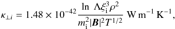 (21)while the conductivity of neutrals is given by,
  (22)The heat-loss function, L, depends on the local plasma parameters, and is written as the difference between optically thin radiative losses (Hildner 1974) and a heating term. Then, our heat-loss function can be expressed as,
 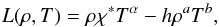 (23)with χ∗ and α being piecewise functions depending on the temperature (Hildner 1974). For an optically thin plasma, radiative cooling may not be fully justified in prominence conditions, or at least for its most internal regions, because they tend to be optically thick. In this case, radiative losses are greatly reduced which can be represented by changing the exponent α in the cooling function, for temperatures T ≤ 104 K, as well as by changing χ∗ accordingly (Milne et al. 1979; Rosner et al. 1978; Carbonell et al. 2004). The last term in Eq. (23) represents an arbitrary heating function which can be modified by taking different values for the exponents a and b.
Finally, the general expression for the viscous heating in terms of the viscosity tensor (Braginskii 1965) is, 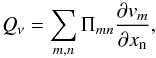 (24)where vm is the mth component of the velocity vector, and xn is the nth coordinate, while the components of Πmn are expressed in terms of the components of the stress tensor Wαβ.
4. Background plasma
The background state can be described as follows:  (25)where T0, p0, ρ0, B0, and v0 are the background temperature, plasma pressure, density, magnetic field and velocity, respectively, and we assume a constant density and no background flow. Then, Eqs. (1)–(5) become:
 ![Mathematical equation: \begin{eqnarray} &&\rho_0 = {\rm const.}, \ \vec v_0 = 0, \ \nabla p_0=0, \ p_0 = \frac{\rho_0 R T_0}{\tilde \mu}, \nonumber \\ &&\rho_0 \left[R\left(\frac{1}{\tilde \mu} \frac{\partial T_0}{\partial t}+T_0 \frac{\partial}{\partial t}\left(\frac{1}{\tilde \mu}\right)\right)+\frac{2}{3} \frac{\chi}{H}\frac{\partial}{\partial t}\left(\frac{1}{\tilde \mu}-1\right)\right]= -\frac{2}{3}\cal L, \label{hetacool} \end{eqnarray}](/articles/aa/full_html/2018/01/aa31567-17/aa31567-17-eq76.png) (26)where
(26)where  since j0 = 0, and thermal conduction is absent because temperature is time-dependent only, and we have neglected viscous heating. In the energy equation (Eq. (26)), the interplay between optically thin radiation, heating, and temporal evolution of the mean atomic weight , due ionization or recombination processes taking place in the plasma, determines how the background temperature evolves with time.
Although the assumption of LTE is not fully realistic for prominence conditions, for the sake of simplicity, we compute the temporal variation of the mean atomic mass, , by means of the Saha equation which for a hydrogen plasma can be written as (Hansen et al. 2004), ![Mathematical equation: \begin{equation} \frac{n_{\rm i}^2 (t)}{n_{\rm n}(t)} =\left(\frac{2 \pi m_{\rm e} k_{\rm B} T_0 (t)}{h^2}\right)^{3/2} \exp \left[-\frac{\chi}{k_{\rm B} T_0 (t)}\right], \label{saha} \end{equation}](/articles/aa/full_html/2018/01/aa31567-17/aa31567-17-eq79.png) (27)where ni(t) and nn(t) are the time-dependent ion and neutral-number densities, me is the electron mass, kB is the Boltzmann’s constant, h is the Planck’s constant, and χ = 13.6 eV is the hydrogen ionization potential. From Eq. (27), we compute ξi and ξn as functions of density and temperature as,
(27)where ni(t) and nn(t) are the time-dependent ion and neutral-number densities, me is the electron mass, kB is the Boltzmann’s constant, h is the Planck’s constant, and χ = 13.6 eV is the hydrogen ionization potential. From Eq. (27), we compute ξi and ξn as functions of density and temperature as,  where
where  (30)with
  (31)Then, using Eqs. (8) and (28), the mean atomic weight can be expressed as,
  (32)Another parameter, which also varies with time, is the electron number density whose expression can be obtained from the Saha equation, and is given by
 ![Mathematical equation: \begin{equation} n_{\rm e} (t) = \frac{\xi_{\rm n}(t)}{\xi_{\rm i}(t)}\left(\frac{2 \pi m_{\rm e} k_{\rm B} T_0 (t)}{h^2}\right)^{3/2} \exp \left[-\frac{\chi}{k_{\rm B} T_0 (t)}\right]\cdot \end{equation}](/articles/aa/full_html/2018/01/aa31567-17/aa31567-17-eq92.png) (33)To obtain the temporal variation of the temperature when the plasma is heated or cooled, we substitute Eq. (32) in (26), and we start from a background equilibrium with constant temperature. Next, we produce an imbalance between the radiative and heating terms giving a value to the constant h. This value for h is determined in the following way: in the case of heating, we assume the initial temperature to be 4000 K, at which the plasma is almost neutral (ξi ~ 0.0004), and we impose a final temperature of 9000 K, at which the plasma is almost fully ionized (ξi ~ 0.9994); while in the case of cooling, temperature varies from 9000 K to 4000 K. Next, since radiation increases or decreases with the temperature, when the plasma attains the assumed final temperature, radiative and heating terms become equal and setting the heat-loss function equal to zero, the constant h can be obtained from
(33)To obtain the temporal variation of the temperature when the plasma is heated or cooled, we substitute Eq. (32) in (26), and we start from a background equilibrium with constant temperature. Next, we produce an imbalance between the radiative and heating terms giving a value to the constant h. This value for h is determined in the following way: in the case of heating, we assume the initial temperature to be 4000 K, at which the plasma is almost neutral (ξi ~ 0.0004), and we impose a final temperature of 9000 K, at which the plasma is almost fully ionized (ξi ~ 0.9994); while in the case of cooling, temperature varies from 9000 K to 4000 K. Next, since radiation increases or decreases with the temperature, when the plasma attains the assumed final temperature, radiative and heating terms become equal and setting the heat-loss function equal to zero, the constant h can be obtained from 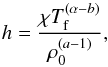 (34)where Tf is the final temperature and, for our calculations, it has been assumed that a = b = 0, corresponding to a constant heating per unit volume. Other values for a and b do not introduce significant differences in the computed temperature profiles.
 |
Fig. 1 Temperature vs. time for the cooling (red line) and heating (blue line) processes. In all the plots, the initial temperature for the heating process is 4000 K and the final temperature is 9000 K, while in the cooling process, the initial and final temperatures are 9000 K and 4000 K, respectively. Furthermore, from now on, in all the plots optically thin radiation has been considered as well as the same constant density value, ρ = 5 × 10-11 kg m-3. |
 |
Fig. 2 Specific internal energy, e, vs. time for the cooling (left panel) and heating (right panel) processes. Internal energy is represented by red lines, ionization potential energy by blue lines, and both terms together by black lines. |
 |
Fig. 3 Relative density of ions, ξi (left panel) and neutrals, ξn (right panel) vs. time, for cooling (red lines) and heating (blue lines) processes. |
 |
Fig. 4 Logarithms of Spitzer’s resistivity, η (left panel), and of Cowling’s resistivity, ηC (right panel) vs. time, for cooling (red lines) and heating (blue lines) processes. |
Following the procedure described above, and once Eq. (32) has been substituted in Eq. (26), we numerically solve Eq. (26) to obtain the temporal variation of the temperature when the prominence plasma is cooled from 9000 K to 4000 K or heated from 4000 K to 9000 K. During the previously described processes, we consider that all the energy supplied to or removed from the plasma is invested into producing more ions (ionization process) or neutrals (recombination process), while the excitations of atoms are neglected.
Figure 1 displays the temporal behaviour of the temperature profile when the plasma is cooled or heated and optically thin radiation is considered. In this figure, and as we have explained before, we observe that, initially, when the plasma is heated, the slope of the temperature increase is very steep; later, while the ionization degree changes, that is, when part of the energy injected into the plasma is invested in increasing the ionization degree, this slope becomes less steep and, once the plasma becomes almost fully ionized, the slope of the temperature increase becomes steeper until the final temperature is attained. When the plasma is cooled, the slope of the temperature decrease is, initially, very steep, however, when recombination processes start, energy is poured into the plasma and the effect is that the slope of the temperature decrease becomes less steep until the plasma becomes almost neutral and the final temperature is reached. As can also be observed in Fig. 1, the time needed to heat the plasma up to its final temperature is much shorter than for the cooling process in agreement with the observational results obtained by Soru-Escaut & Mouradian (1990). The presence of the ionization potential energy term in the specific internal energy helps to properly describe the physical processes taking place in the plasma since the temporal evolution of this term, involving the ionization degree, represents an extra energy sink or source for the plasma.
For the cooling and heating processes, and in the case of optically thin radiation, Fig. 2 displays the temporal behaviour of the two terms involved in the specific internal energy as well as of the total specific internal energy. It shows that for a plasma whose physical conditions are akin to those of a prominence plasma, the term corresponding to the ionization potential energy cannot be neglected at all since when the plasma temperature evolves with time, and the ionization degree changes, this term represents a strong contribution to the total specific internal energy. Furthermore, we can observe that in the cooling process, this term almost goes to zero, and the specific internal energy becomes constant when the plasma becomes almost neutral, while in the heating process this term starts from almost zero and the specific internal energy becomes almost constant when the plasma becomes almost fully ionized. Therefore, taking into account the term of ionization potential energy in the specific internal energy (Eq. (14)), which has sometimes been disregarded (Leake & Arber 2006), could be extremely important depending on the temporal evolution of the ionization degree and the physical properties of the considered plasma. Finally, Figs. 3 and 4 show the temporal variation of microscopic plasma parameters such as the relative densities of ions and neutrals and the Cowling’s and Spitzer’s resistivities, respectively, when the plasma is heated or cooled, and for the case of optically thin radiation. As can be seen in Fig. 4, Cowling’s resistivity, dominated by ion-neutrals collisions, is much greater than Spitzer’s resistivity, due to ion-electron collisions, and its temporal behaviour, during heating or cooling processes, can be understood from Eq. (10). During the cooling process, the first term in Eq. (10), which describes Spitzer’s resistivity, increases, while the second term also increases because of the interplay between the relative density of neutrals, ξn, and the neutral friction coefficient, αn. The opposite happens during the heating process. When the efficiency of radiative losses is reduced ad hoc in order to approximately represent optically thick radiation, the behaviour of the temperature profile as well as of the different plasma parameters is similar, with the only difference being that a longer time is needed to reach the final constant value.
5. Linear wave equations
Next, we impose small perturbations on the background state and we describe the temporal and spatial behaviour of these perturbations as f1(x,z,t) = f1(t)eikxxeikzz with f1(t) being the time dependent amplitude of the perturbations, and kx, kz the wavenumbers in the direction parallel and perpendicular to the magnetic field. Then, the time dependent linear wave equations for coupled slow and fast MHD waves are, 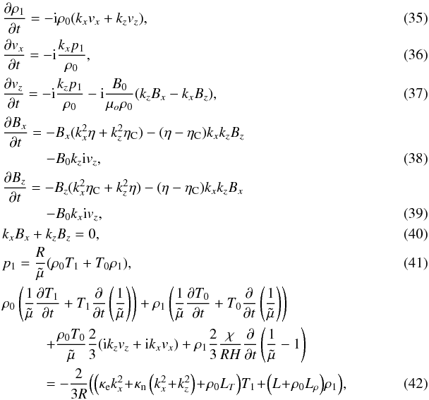 while for Alfvén waves we obtain,
  where ρ1, T1, p1, Bx, By, Bz, vx, and vyvz represent density, temperature, pressure, magnetic field, and velocity perturbations, respectively. The last two equations can be combined to give,
  (45)which describes the temporal behaviour of the perturbed velocity amplitude of the Alfvén wave. In this equation,
  is the squared Alfvén speed given by,
  (46)which is constant in time, while η and ηC are time-dependent functions.
Since our main interest is to describe the temporal behaviour of MHD waves in a plasma whose temperature changes with time, we are going to consider Alfvén, slow, and fast waves separately.
6. Alfvén waves
Let us consider only parallel propagation (kx ≠ 0, kz = 0) to the magnetic field, In this case, and as can be obtained from Eq. (45), the equation to be solved is,  (47)where dissipation is only due to the time dependent Cowling’s resistivity. We use the WKB method (Bender & Orszag 1978) to seek an approximate analytical solution to Eq. (47). To this end, we define a dimensionless time t′ = t/τ, where τ can be related to the cooling or heating time. Then, we assume that the perturbed velocity can be written as,
  (48)where A(t′) is the amplitude. The condition of applicability of the WKB approximation is that P/τ ≪ 1, where P is the period of the wave. After performing the corresponding substitutions in Eq. (47) and considering only terms of order τ0 and τ-1, we are left with the following equations,
 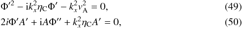 where ′ means the temporal derivative. Once solved, these equations provide solutions for the functions Φ and A, which expressed in terms of the original temporal variable, t, are,
 ![Mathematical equation: \begin{eqnarray} &&\Phi(t) = \frac{1}{2} \left[{\rm i} k_x^2 \int \eta_{\rm C} (t) {\rm d}t \pm \int \sqrt{\left(4 k_x^2 v_{\rm A}^2-k_x^4 \eta_{\rm C} (t)^2\right)} {\rm d}t \right], \label{fig:wkb001} \\ &&A(t) = C \ \exp \left[-\int\frac{\Phi^{\prime\prime}(t) \left(\Phi^{\prime}(t) + {\rm i} \eta_{\rm C} (t) k_x^2\right)}{4 \Phi^{\prime2}(t)(t)+k_x^4 \eta_{\rm C}^2(t)}{\rm d}t\right] , \label{fig:wkb02} \end{eqnarray}](/articles/aa/full_html/2018/01/aa31567-17/aa31567-17-eq135.png) with C being a constant, and the perturbed velocity being given by,
with C being a constant, and the perturbed velocity being given by, ![Mathematical equation: \begin{equation} v_y(t) = A(t) \exp \left[{\rm i} \Phi(t)\right]. \end{equation}](/articles/aa/full_html/2018/01/aa31567-17/aa31567-17-eq137.png) (53)When ηC = 0, that is, a fully ionized non-resistive plasma, we are left with
(53)When ηC = 0, that is, a fully ionized non-resistive plasma, we are left with  which describes a propagating undamped Alfvén wave whose velocity perturbation is given by vy(t) = Cexp[ikxvAt]. When ηC = const., that is, a partially ionized plasma with constant temperature, we obtain
 ![Mathematical equation: \begin{equation} \Phi(t) = \frac{1}{2} \left[{\rm i} k_x^2 \eta_{\rm C} \pm \sqrt{\left(4 k_x^2 v_{\rm A}^2-k_x^4 \eta_{\rm C} ^2\right)} \right] t, \label{fig:wkb04} \end{equation}](/articles/aa/full_html/2018/01/aa31567-17/aa31567-17-eq142.png) (56)and the perturbed velocity is given by,
(56)and the perturbed velocity is given by, ![Mathematical equation: \begin{equation} v_y(t) = C \exp \left[- \frac{1}{2} k_x^2 \eta_{\rm C} t \right] \exp\left[ \pm \frac{\rm i}{2} \sqrt{\left(4 k_x^2 v_{\rm A}^2-k_x^4 \eta_{\rm C}^2\right)} t \right], \label{fig:wkb05} \end{equation}](/articles/aa/full_html/2018/01/aa31567-17/aa31567-17-eq143.png) (57)describing, in principle, a damped propagating Alfvén wave. However, previous studies about the propagation of Alfvén waves in partially ionized plasmas using the single-fluid approximation have pointed out the presence of cut-off wavenumbers (Forteza et al. 2008; Zaqarashvili et al. 2012). The presence of a cut-off wavenumber means that waves with a wavenumber higher than the cut-off wavenumber are evanescent, that is, the frequency becomes imaginary. A physical interpretation of the presence of these cut-off wavenumbers was provided by Soler et al. (2013) in terms of the tension and friction forces, and when both forces are balanced the velocity perturbation becomes evanescent. In the case of Alfvén waves, and for a constant temperature, the expression for the cut-off wavenumber is (Forteza et al. 2008),
(57)describing, in principle, a damped propagating Alfvén wave. However, previous studies about the propagation of Alfvén waves in partially ionized plasmas using the single-fluid approximation have pointed out the presence of cut-off wavenumbers (Forteza et al. 2008; Zaqarashvili et al. 2012). The presence of a cut-off wavenumber means that waves with a wavenumber higher than the cut-off wavenumber are evanescent, that is, the frequency becomes imaginary. A physical interpretation of the presence of these cut-off wavenumbers was provided by Soler et al. (2013) in terms of the tension and friction forces, and when both forces are balanced the velocity perturbation becomes evanescent. In the case of Alfvén waves, and for a constant temperature, the expression for the cut-off wavenumber is (Forteza et al. 2008),  (58)where the + and – signs refer to parallel and anti-parallel propagation with respect to the magnetic field direction, and θ is the propagation angle with respect to the magnetic field. Therefore, when only parallel propagation is considered, the above expression becomes,
  (59)which can obtained from Eq. (57) by making the expression in the parenthesis inside the bracket of the second exponential factor equal to zero. In our case, since the temperature changes with time, Eq. (59) could not be suitable and would need to be modified. Then, we could follow a similar approach by making the parenthesis inside the second integral of Eq. (51) equal to zero to obtain an approximation to the cut-off wavenumber such as,
 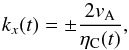 (60)whose only difference with Eq. (59) is the temporal dependence of Cowling’s resistivity. Equation (60) points out that in this case the cut-off wavenumber is not constant but time dependent because of the temporal dependence of Cowling’s resistivity. For instance, during the cooling process the value of the cut-off wavenumber decreases because Cowling’s resistivity increases while, inversely, during the heating process its value increases because Cowling’s resistivity decreases, and both temporal behaviours are shown in Fig. 5. Up to now, the observed wavenumbers in small-amplitude prominence oscillations are in the range 10-6−10-7 m-1 (see Arregui et al. 2012), which means that they are always smaller than the cut-off wavenumbers for Alfvén waves shown in Fig. 5.
 |
Fig. 5 Temporal behaviour of the cut-off wavenumber during cooling (red line) and heating (blue line) processes. |
 |
Fig. 6 Cooling case. Left panel: logarithms of twice the Alfvén speed, 2va, (blue line) and ηCkx (red line) vs. time. Right panel: evanescent behaviour of the Alfvén velocity amplitude (kx = 5 m-1). The velocity amplitude has been normalized. |
 |
Fig. 7 Cooling case. Left panel: logarithms of twice the Alfvén speed, 2va, (blue line) and ηCkx (red line) vs. time. Right panel: real part of the frequency vs. time (kx = 10-6 m-1). |
 |
Fig. 8 Heating case. Left panel: logarithms of twice the Alfvén speed, 2va, (blue line) and ηCkx (red line) vs. time. Right panel: evanescent behaviour of the Alfvén velocity amplitude (kx = 5 × 10⁻⁶ m-1). The velocity amplitude has been normalized. |
In the case of a cooling process, Fig. 6 shows the effect of the cut-off wavenumber. In the left panel, the term ηC(t)kx is always greater than twice the constant Alfvén speed, vA, because of the chosen wavenumber, therefore, the frequency is always imaginary, such as can be derived from Eq. (51), and the Alfvén wave once excited becomes evanescent immediately, as seen in Fig. 6 (right panel). The evanescent behaviour of the perturbations excited at t = 0 with wavenumbers greater than the cut-off wavenumber means that these perturbations cannot propagate away from the place of the excitation in the form of travelling waves. However, all the energy stored in the perturbation is immediately dissipated, heating the plasma. This behaviour of the Alfvén velocity amplitude has been obtained by numerically solving Eq. (47) with kx = 5 m-1, kz = 0 together with the initial conditions vy(0) = 1,  . On the contrary, in Fig. 7 (left panel) twice the Alfvén speed and the term ηC(t)kx become equal for a time t ~ 23 000 s, at which the frequency becomes imaginary and the Alfvén wave would become evanescent. Figure 7 (right panel) shows the temporal behaviour of the real part of the approximate frequency which becomes zero at the above mentioned time. In the case of a heating process, the left panel of Fig. 8 shows the case in which the term ηC(t)kx is initially greater than twice the constant Alfvén speed, vA, because of the chosen wavenumber, therefore, the frequency is imaginary and the Alfvén wave once excited becomes evanescent immediately, as can be seen in Fig. 8 (right panel). For t> 5 s, ηC(t)kx becomes smaller than twice the constant Alfvén speed, vA, and the frequency becomes real. However, despite the frequency becoming real, the wave needs to be re-excited in order to propagate. The temporal behaviour of the real part of the approximate frequency is shown in Fig. 9 which points out that the frequency starts to be real close to t ~ 5 s. Finally, in the heating case it is not possible to have ηC(t)kx always greater than twice the constant Alfvén speed, vA, because, as can be seen in Fig. 4, Cowling’s resistivity decreases very rapidly and we would need an extremely large and completely unphysical value for the wavenumber. These results confirm our previous analysis about the presence of cut-off wavenumbers based on the WKB approximation.
On the other hand, from Eq. (51) we can also obtain further information about the damping time and the oscillatory period of the Alfvén wave. From the first exponential in Eq. (57), and since we have a time-dependent Cowling’s resistivity, the damping time, τD, could be approximated by,  (61)which implies a time dependent damping time because of Cowling’s resistivity. Furthermore, from the second exponential in Eq. (57), the approximated expression for the oscillatory period, P, would be,
 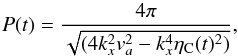 (62)which is also time dependent because of Cowling’s resistivity.
Next, and considering only parallel propagation to the magnetic field (kx = 10-6 m-1,kz = 0), we numerically solved Eq. (47) together with the initial conditions vy(0) = 1, . The chosen value for the parallel wavenumber corresponds to a typical observed wavelength in prominence oscillations. Figure 10 (left panel) displays a comparison of the Alfvén velocity amplitude for the cooling and heating cases, showing the different behaviour of the damping, which is determined by the temporal behaviour of Cowling’s resistivity. In the cooling case (red line), and for the wavenumber considered, the Alfvén wave suffers an initial weak attenuation. However, this attenuation increases with time, because of the temporal behaviour of Cowling’s resistivity, and the wave is almost completely attenuated around t ~ 15 000 s. From a physical point of view, at the beginning of the cooling process, the neutrals density is very small, which implies a very long damping time (see Fig. 12 right panel), but, as time goes by, neutrals density increases and the damping time slowly decreases. It is worth mentioning here that in Fig. 7 (left panel) at t ~ 23 000 s, and taking into account Eq. (58), the horizontal wavenumber becomes kx = 10-6 m-1, that is, the cut-off wavenumber coincides with the parallel wavenumber used in our computations and, therefore, the Alfvén wave should become evanescent. However, as stated before, around t ~ 15 000 s the wave has been completely attenuated and, consequently, the cut-off wavenumber does not play any role in this case.
 |
Fig. 9 Heating case: real part of the frequency vs. time (kx = 5 × 10⁻⁶ m-1). |
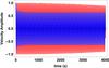 |
Fig. 10 Comparison of the Alfvén wave velocity amplitude vs. time for the cooling (red line) and heating (blue line) processes. kx = 10-6 m-1. The velocity amplitude has been normalized. |
On the contrary, for the heating case (blue line), and as is shown in Fig. 10 (left panel), the velocity amplitude is initially strongly attenuated because Cowling’s resistivity at the initial temperature has a very high value, but it decreases rapidly and when the plasma becomes almost fully ionized at the final temperature, this resistivity attains a constant and much smaller value than at the initial temperature. Then, the second term in Eq. (47) becomes very small and the Alfvén wave becomes almost undamped. In order to have a more strong damping, we would need to increase the wavenumber up to a very unphysical value. In this case, initially, we have a very high density of neutrals, which explains the strong damping; however, due to the fast increase of the temperature, neutrals density quickly decreases and damping time becomes longer. This quite different behaviour between the heating and cooling cases is produced by the different profile of the increase/decrease of Cowling’s resistivity which depends on the temporal behaviour of several parameters, as shown in Eq. (10), although the numerical value of the horizontal wavenumber is also important because of its presence in the second term of Eq. (47).
Next, we performed a comparison of the Alfvén wave velocity amplitudes for three different cases: a plasma which is heated or cooled with T0(t); an almost neutral plasma with T0 = 5000 K and ξi = 0.02, and an almost fully ionized plasma with T0 = 8000 K and ξi = 0.99. The main effect influencing the behaviour of Alfvén wave velocity amplitude is the temporal behaviour of Cowling’s resistivity. Since for T = 8000 K, the numerical value of Cowling’s resistivity is, in general, much smaller than in the other two cases, in both panels of Fig. 11 we have only plotted the cases corresponding to T0(t) and T0 = 5000 K. This comparison points out that the Alfvén wave velocity amplitude is strongly attenuated in the case of an almost neutral plasma, as should be expected, because its Cowling’s resistivity is much greater, at least during the major part of the time interval considered, than for the plasma undergoing heating or cooling.
Finally, in Fig. 12 we have plotted, for a fixed wavenumber, the temporal behaviour of the logarithm of the approximated damping time (see Eq. (61)). We observe that in the cooling case, initially, the damping time is very long, because Cowling’s resistivity is small, and therefore the damping is weak, but later on, Cowling’s resistivity increases and the damping time decreases becoming constant when Cowling’s resistivity becomes constant, and therefore the attenuation becomes stronger. In the heating case, the opposite happens; the damping time is very short at the beginning, since Cowling’s resistivity is high, and therefore the wave is initially strongly attenuated, but later on the damping time increases, becoming constant, and the attenuation is very weak, as can be seen in Fig. 10. Regarding the period, in the cooling case, initially, and since Cowling’s resistivity is small, the period is basically coincident with that of an ideal Alfvén wave,  . Later on, the period starts to increase rapidly, since, due to the increase of Cowling’s resistivity, the denominator becomes smaller. In the heating case, Cowling’s resistivity is initially very high, and therefore, from Eq. (62), the period is longer than for the cooling case, but later, and since the resistivity decreases rapidly, becoming constant, the period also becomes constant and coincident with that of a pure Alfvén wave.
 |
Fig. 11 Alfvén wave velocity amplitude vs. time. Left panel: plasma cooled from T0(t) = 9000 K to 4000 K (red line); partially ionized plasma with T0 = 5000 K and ξi = 0.02 (blue line). Right panel: plasma heated from T0(t) = 4000 K to 9000 K (red line); partially ionized plasma with T0 = 5000 K and ξi = 0.02 (blue line; kx = 10-6 m-1). The velocity amplitude has been normalized. |
In summary, the approximated expressions for the damping time and period derived from the WKB approximation are in full agreement with the numerical results obtained for the temporal behaviour of the Alfvén velocity amplitude. On the other hand, from Eq. (47), and assuming that the velocity amplitude behaves like vy ~ eiωt, an approximated expression for a modified Alfvén speed can be obtained, which is given by,  (63)which is a time-dependent complex Alfvén speed. Using this modified Alfvén speed, we could write a dispersion relation for Alfvén waves such as,
 (64)and from it, the expressions for the damping time and period are fully coincident with Eqs. (61) and (62) derived from the WKB approximation. Furthermore, using Γa = Γr + iΓi, with Γr and Γi, the real and imaginary parts of the modified Alfvén speed, respectively, we could also write the velocity perturbation such as,
 (65)which suggests that we could write an expression such as
  representing a damping timescale. Comparing this expression with Eq. (57), we would conclude that
  .
.
 |
Fig. 12 Temporal behaviour of the logarithm of damping time for the Alfvén wave in the cooling (red line) and heating (blue line) processes (kx = 10-6 m-1). |
7. Slow waves
In this Section, we study the temporal behaviour of slow waves in a background plasma whose temperature changes with time. In the case of parallel propagation, from Eqs. (35), (36), (41), and (42), we can derive a single differential equation for the perturbed velocity amplitude, vx, which is, ![Mathematical equation: \begin{eqnarray} &&\frac{\partial^2 v_x}{\partial t^2} + k_x^2 c_{\rm s}^2 v_x = \frac{2}{3}\left[ \frac {\rho_1 \chi}{\rho_0 H}\frac{\partial}{\partial t}\left(\frac{1}{\tilde \mu}-1\right) \right] {\rm i} k_x \nonumber \\ &&\qquad\qquad\qquad\quad+ \frac{2}{3} \left[\frac{\left(\kappa_{\rm e} k_x^2+\kappa_{\rm n} k_x^2 + \rho_0 L_{T} \right) T_1}{\rho_0} \right] {\rm i} k_x \nonumber \\ && \qquad\qquad\qquad\quad+ \frac{2}{3} \left[\frac{\left(L+\rho_0 L_{\rho} \right) \rho_1}{\rho_0}\right] {\rm i} k_x, \label{gral_slow} \end{eqnarray}](/articles/aa/full_html/2018/01/aa31567-17/aa31567-17-eq193.png) (66)which points out that the damping of slow waves is not affected by resistivities, but only by thermal effects. From Eq. (66), an analytical solution for the perturbed velocity, vx, cannot be obtained. Therefore, we have numerically solved Eqs. (35)–(42) with the initial conditions: vx(0) = 1, vz(0) = ρ1(0) = T1(0) = Bx(0) = Bz(0) = 0, together with kx = 10-6 m-1, kz = 0, and we have studied the effect of heating and cooling processes on the temporal behaviour of the velocity amplitude of slow waves.
(66)which points out that the damping of slow waves is not affected by resistivities, but only by thermal effects. From Eq. (66), an analytical solution for the perturbed velocity, vx, cannot be obtained. Therefore, we have numerically solved Eqs. (35)–(42) with the initial conditions: vx(0) = 1, vz(0) = ρ1(0) = T1(0) = Bx(0) = Bz(0) = 0, together with kx = 10-6 m-1, kz = 0, and we have studied the effect of heating and cooling processes on the temporal behaviour of the velocity amplitude of slow waves.
Figure 13 shows a comparison between three different situations: A plasma which is cooled or heated between 4000 K and 9000 K; an almost fully ionized plasma with constant temperature T0 = 8000 K and ξi = 0.99, and an almost neutral plasma with constant temperature T0 = 5000 K and ξi = 0.02. In the cooling case (Fig. 13, left panel), the damping time and the period of the slow wave in the almost fully ionized plasma with constant temperature and of the damping time and the period of the plasma suffering the cooling process are very similar. For the almost neutral plasma with constant temperature, however, the period is longer and the attenuation weaker. In the heating case (Fig. 13, right panel), the period of the slow wave is different in the three considered plasmas while attenuation is stronger for the almost fully ionized plasma than for the heated plasma, and is weaker for the almost neutral plasma.
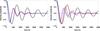 |
Fig. 13 Slow-wave velocity amplitude vs. time. Left panel: plasma cooled from T0(t) = 9000 K to 4000 K (red line); almost fully ionized plasma with T0 = 8000 K and ξi = 0.99 (blue line); almost neutral plasma with T0 = 5000 K and ξi = 0.02 (black line). Right panel: plasma heated from T0(t) = 4000 K to 9000 K (red line); almost fully ionized plasma with T0 = 8000 K and ξi = 0.99 (blue line); almost neutral plasma with T0 = 5000 K and ξi = 0.02 (black line; kx = 10-6 m-1). The velocity amplitude has been normalized. |
 |
Fig. 14 Left panel: slow-wave period vs. time for plasma cooled from T0(t) = 9000 K to 4000 K (red line); almost fully ionized plasma with T0 = 8000 K and ξi = 0.99 (blue line); almost neutral plasma with T0 = 5000 K and ξi = 0.02 (black line). Right panel: slow-wave damping time vs. time for plasma cooled from T0(t) = 9000 K to 4000 K (red line); almost fully ionized plasma with T0 = 8000 K and ξi = 0.99 (blue line); almost neutral plasma with T0 = 5000 K and ξi = 0.02 (black line; kx = 10-6 m-1). |
In order to have a quantitative understanding of the above described features, from Eqs. (41) and (42), and assuming that the perturbed pressure and density behave like p1,ρ1 ~ eiωt, we can obtain an approximate expression for the nonadiabatic sound speed, Λs, which is given by, 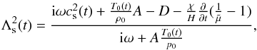 (67)with,
 which means that we have a complex and time-dependent nonadiabatic sound speed. This expression is different from that corresponding to the nonadiabatic sound speed in a fully or partially ionized plasma with constant temperature (Forteza et al. 2008; Soler et al. 2008; Carbonell et al. 2009) because of the presence of the fourth member in the numerator, which accounts for the temporal variation of the mean atomic weight due to ionization/recombination processes, together with the time-dependent thermal terms. In the adiabatic case and for constant temperature, Eq. (67) becomes the adiabatic sound speed,
  . Using this expression for Λs, we can write an approximate WKB-like dispersion relation for slow waves given by,
  (70)then, solving this equation, we obtain two complex solutions corresponding to slow waves and a purely imaginary solution corresponding to a thermal or entropy wave. From the complex solutions for ω, we can obtain the wave period given by
  and the damping time given by
  , where ωr(t) and ωi(t) are the real and imaginary parts of ω(t), respectively. As in the case of Alfvén waves, using Λa = Λr + iΛi, with Λr and Λi, the real and imaginary parts of the nonadiabatic sound speed, respectively, we could also write the velocity perturbation such as,
 (71)which suggests that we could write an expression such as
  representing the same damping timescale as before, written in terms of the imaginary part of the nonadiabatic sound speed.
Figure 14 (left panel) shows, for the cooling case, a comparison between the periods of the slow waves in a cooled plasma, in an almost fully ionized plasma, and in an almost neutral plasma. The periods for the almost fully ionized plasma and almost neutral plasma are obtained from the nonadiabatic sound speed with constant temperature and are constant, as must be expected; however, for the cooled plasma, the period varies with time, showing an initial decrease, although after a short time it starts to increase approaching the value of the period for the almost fully ionized plasma at T0 = 8000. Furthermore, from this plot we can see why, in Fig. 13 (left panel) and during the time interval considered, the slow wave has a similar period in the cooled plasma and in the almost fully ionized plasma, while the period is much longer in an almost neutral plasma. Figure 14 (right panel) shows a similar comparison but for damping times and it can be seen that the damping times for the cooled plasma and the almost fully ionized plasma are very similar, at least during the time interval considered, which explains the more or less simultaneous damping of the oscillation in both plasmas observed in Fig. 13 (left panel), while for an almost neutral plasma the damping time is much longer, as shown in Fig. 14 (right panel). Following the same procedure, the behaviour of the slow-wave period and damping time in the heated plasma, as compared with that of almost neutral and fully ionized plasmas, can be understood. At the beginning, the slow-wave period in the heated plasma is greater than in the almost fully ionized plasma, as observed in Fig. 13 (right panel), but after a short time it starts to decrease, approaching the value of the slow-wave period in the almost fully ionized plasma. Regarding the damping time, initially it is greater than for an almost fully ionized plasma, but later on it decreases attaining a value similar to that of the almost fully ionized plasma; this behaviour can also be observed in Fig. 13 (right panel). Next, Fig. 15 shows, for a heated/cooled plasma, a comparison of the slow-wave velocity amplitude, which highlights the difference in period and damping time between both cases.
 |
Fig. 15 Comparison of the slow-wave velocity amplitude vs. time for the cooling (red line) and heating (blue line) processes (kx = 10-6 m-1). The velocity amplitude has been normalized. |
Ballester et al. (2016) analyzed the temporal behaviour of slow waves in a fully ionized plasma undergoing heating or cooling processes. In this analysis, the temporal variation of the temperature profile was computed from the energy equation, in which it was assumed that radiative losses were proportional to the temperature, obtaining exponentially increasing or decreasing temperature profiles. In the case of the studied slow waves, the most important differences with respect to the results reported here are related with the nonadiabatic sound speed, period, and damping time. In our case, the nonadiabatic sound speed involves thermal terms such as optically thin radiation, thermal conduction by electrons and neutrals, and the temporal variation of the ionization degree; therefore, its expression is completely different, and more realistic, than in Ballester et al. (2016). Using the nonadiabatic sound speed, the temporal variation of the period and damping time can be obtained, and they are very different from those in Ballester et al. (2016). In particular, the damping time is much shorter in the case of the heated/cooled partially ionized plasma, because radiative losses and thermal conduction are more efficient than in the case of a heated/cooled fully ionized plasma, and the period does not behave as an exponentially increasing or decreasing function as in a heated/cooled fully ionized plasma.
In the case of slow and fast waves in prominence and coronal conditions, wave and thermal instabilities can be followed using two instability criteria (Field 1965; Carbonell et al. 2004), which, applied to our case, can be written as:  (72)for the isentropic criterion describing wave instability, and
  (73)for the isobaric criterion describing thermal instability. Using our results for slow waves, none of these criteria are satisfied, and therefore neither wave nor thermal instabilities are present.
 |
Fig. 16 Comparison of the fast wave velocity amplitude vs. time for the cooling (red line) and heating (blue line) processes (kz = 10-6 m-1). The velocity amplitude has been normalized. |
 |
Fig. 17 Fast wave velocity amplitude vs. time. Left panel: plasma cooled from 9000 K to 4000 K (red line); almost neutral plasma with T = 5000 K and ξi = 0.02 (blue line). Right panel: plasma heated from 4000 K to 9000 K (red line); almost neutral plasma with T = 5000 K and ξi = 0.02 (blue line; kz = 10-6 m-1). The velocity amplitude has been normalized. |
8. Fast waves
In this section we study the temporal behaviour of fast waves when the plasma is heated or cooled. From Eqs. (35), (37)–(39), (41), and (42), and in the case of perpendicular propagation, (kx = 0, kz ≠ 0), we can derive a single differential equation for the perturbed velocity amplitude, vz, which is, ![Mathematical equation: \begin{eqnarray} &&\frac{\partial^2 v_z}{\partial t^2} + k_z^2 \left(c_{\rm s}^2 + v_{\rm a}^2\right) v_z = \frac{2}{3} \left[ \frac {\rho_1 \chi}{\rho_0 H}\frac{\partial}{\partial t}\left(\frac{1}{\tilde \mu}-1\right) \right] {\rm i} k_z \nonumber \\ &&\qquad\qquad\qquad+ \frac{2}{3} \left[\frac{\left(\kappa_{\rm n} k_z^2 + \rho_0 L_{\rm T}\right) T_1}{\rho_0} \right] {\rm i} k_z \nonumber \\ &&\qquad\qquad\qquad+ \frac{2}{3} \left[\frac{\left(L+\rho_0 L_{\rho}\right) \rho_1}{\rho_0}\right] {\rm i} k_z + {\rm i} v_{_rm a}^2\frac{B_x}{B_0} \eta_{\rm C} k_z^2. \label{gral_fast} \end{eqnarray}](/articles/aa/full_html/2018/01/aa31567-17/aa31567-17-eq221.png) (74)From the above equation we can infer that the damping of fast waves is produced by Cowling’s resistivity together with thermal effects. Since we cannot obtain an analytical solution for the velocity amplitude vz, we have numerically solved Eqs. (35)–(42) with the initial conditions: vz(0) = 1, vx(0) = ρ1(0) = T1(0) = Bx(0) = Bz(0) = 0, together with kx = 0 and kz = 10-6 m-1. Figure 16 displays, for the cooling and heating processes, the temporal behaviour of the fast wave velocity amplitude showing that, in principle, its behaviour seems to be similar to that of Alfvén waves. However, comparing Fig. 16 to Fig. 10 (left panel) we can observe that for the cooling process the behaviour of the velocity amplitude for both waves is very similar because the damping is dominated by the increase of Cowling’s resistivity, while thermal effects do not play a significant role. Conversely, in the case of the heating process, the behaviour of both velocity amplitudes is very different since when Cowling’s resistivity decreases, the last term in the right-hand side of Eq. (74) becomes negligible and thermal effects, coming from the second and third terms, become dominant and are responsible for the final attenuation observed in Fig. 16. The reason is that when the final temperature is attained and plasma becomes almost fully ionized, Cowling’s resistivity becomes small again (see Eq. (10)), and therefore its attenuation effect also becomes small and the damping starts to be dominated by thermal effects. Furthermore, Fig. 17 shows a comparison between the behaviour of the velocity amplitude for a heated or cooled plasma and for an almost neutral plasma with a constant temperature T0 = 5000 K and ξi = 0.02. In both cases, the damping is stronger for the almost neutral plasma since the constant Cowling’s resistivity is much greater than for the heated/cooled plasma during the major part of the time interval in which the cooling/heating processes are taking place. Therefore, the fast wave velocity amplitude in the almost neutral plasma displays a strong attenuation. When the same comparison is performed considering an almost fully ionized plasma at T0 = 8000 K, the small value of Cowling’s resistivity implies that the damping of the fast wave velocity amplitude is very weak and takes place over a very long time. In summary, in the case of perpendicular propagation, the behaviour of the fast wave velocity amplitude is quite similar to that of Alfvén waves when the plasma is cooled, but it behaves in quite a different way when the plasma is heated because of the additional damping due to thermal effects, which become dominant when Cowling’s resistivity attains a small value. On the other hand, using the same criteria for instabilities as for slow waves, fast waves are stable and thermal instabilities are also absent.
(74)From the above equation we can infer that the damping of fast waves is produced by Cowling’s resistivity together with thermal effects. Since we cannot obtain an analytical solution for the velocity amplitude vz, we have numerically solved Eqs. (35)–(42) with the initial conditions: vz(0) = 1, vx(0) = ρ1(0) = T1(0) = Bx(0) = Bz(0) = 0, together with kx = 0 and kz = 10-6 m-1. Figure 16 displays, for the cooling and heating processes, the temporal behaviour of the fast wave velocity amplitude showing that, in principle, its behaviour seems to be similar to that of Alfvén waves. However, comparing Fig. 16 to Fig. 10 (left panel) we can observe that for the cooling process the behaviour of the velocity amplitude for both waves is very similar because the damping is dominated by the increase of Cowling’s resistivity, while thermal effects do not play a significant role. Conversely, in the case of the heating process, the behaviour of both velocity amplitudes is very different since when Cowling’s resistivity decreases, the last term in the right-hand side of Eq. (74) becomes negligible and thermal effects, coming from the second and third terms, become dominant and are responsible for the final attenuation observed in Fig. 16. The reason is that when the final temperature is attained and plasma becomes almost fully ionized, Cowling’s resistivity becomes small again (see Eq. (10)), and therefore its attenuation effect also becomes small and the damping starts to be dominated by thermal effects. Furthermore, Fig. 17 shows a comparison between the behaviour of the velocity amplitude for a heated or cooled plasma and for an almost neutral plasma with a constant temperature T0 = 5000 K and ξi = 0.02. In both cases, the damping is stronger for the almost neutral plasma since the constant Cowling’s resistivity is much greater than for the heated/cooled plasma during the major part of the time interval in which the cooling/heating processes are taking place. Therefore, the fast wave velocity amplitude in the almost neutral plasma displays a strong attenuation. When the same comparison is performed considering an almost fully ionized plasma at T0 = 8000 K, the small value of Cowling’s resistivity implies that the damping of the fast wave velocity amplitude is very weak and takes place over a very long time. In summary, in the case of perpendicular propagation, the behaviour of the fast wave velocity amplitude is quite similar to that of Alfvén waves when the plasma is cooled, but it behaves in quite a different way when the plasma is heated because of the additional damping due to thermal effects, which become dominant when Cowling’s resistivity attains a small value. On the other hand, using the same criteria for instabilities as for slow waves, fast waves are stable and thermal instabilities are also absent.
9. Energy considerations
The total energy density, Ws, of slow waves propagating along the magnetic field is obtained by adding kinetic and thermal energy densities, and is given by  (75)For fast waves propagating perpendicular to the magnetic field, this energy comes from the addition of kinetic, thermal and magnetic energy densities, and is given by
  (76)while for Alfvén waves propagating along the magnetic field, it is obtained by adding kinetic and magnetic energy densities, and is given by
  (77)To understand the temporal behaviour of the slow-wave total energy density, we could start from the linearized continuity, momentum, and energy equations to obtain, after some straightforward manipulations, the following expression:
 ![Mathematical equation: \begin{eqnarray} &&\frac{\partial}{\partial t}\left(\frac{1}{2} \rho_0 v_{x}^2 + \frac{1}{2 \rho_0 c_{\rm s}^2}p_1^2\right) + \frac{\partial}{\partial x}(p_1 v_{x}) = \nonumber \\ &&\qquad- \frac{p_1 \rho_1}{\rho_0 c_{\rm s}^2} \frac{2}{3} \frac{\chi}{H} \frac{\rm d}{{\rm d} t}\left(\frac{1}{\tilde \mu}-1\right) + \frac{p_1^2}{2 \rho_0} \frac{\partial}{\partial t} \left(\frac{1}{c_{\rm s}^2}\right)\nonumber \\ && \qquad-\frac{2}{3} \frac{p_1}{\rho_0 c_{\rm s}^2}\left[\left(\kappa_{\rm e} k_x^2+\kappa_{\rm n} k_x^2 + \rho_0 L_{T} \right) T_1\right] \nonumber \\ && \qquad-\frac{2}{3} \frac{p_1}{\rho_0 c_{\rm s}^2}\left[\left(L+\rho_0 L_{\rho} \right) \rho_1 \right], \label{timebeh} \end{eqnarray}](/articles/aa/full_html/2018/01/aa31567-17/aa31567-17-eq231.png) (78)in which the terms on the left-hand side provide the temporal variation of the wave, total energy density, and the divergence of the wave energy density flux; on the right-hand side, the first term accounts for the temporal variation of the mean atomic weight, the second term comes from the temporal variation of the sound speed, and the third and fourth terms account for radiative and conductive losses, respectively. These terms on the right-hand side represent a source/sink, which account for the generation or removal of the wave energy density per unit time (Goedbloed & Poedts 2004). Therefore, when the right-hand side is positive, the wave energy density increases with time while, when it is negative, the opposite happens. When plasma temperature is kept constant and thermal losses are neglected, the right-hand side member is zero, then, Eq. (78) has the form of a conservation equation, such as
(78)in which the terms on the left-hand side provide the temporal variation of the wave, total energy density, and the divergence of the wave energy density flux; on the right-hand side, the first term accounts for the temporal variation of the mean atomic weight, the second term comes from the temporal variation of the sound speed, and the third and fourth terms account for radiative and conductive losses, respectively. These terms on the right-hand side represent a source/sink, which account for the generation or removal of the wave energy density per unit time (Goedbloed & Poedts 2004). Therefore, when the right-hand side is positive, the wave energy density increases with time while, when it is negative, the opposite happens. When plasma temperature is kept constant and thermal losses are neglected, the right-hand side member is zero, then, Eq. (78) has the form of a conservation equation, such as  , with Π being the energy flux, and the wave energy density remains constant in time. On the other hand, while radiative and conductive losses are always sinks of energy, the temporal behaviour of the first and second terms on the right-hand side changes when a heating or cooling process is considered. For instance, the temporal behaviour of the inverse of the squared sound speed, which depends on a time-dependent temperature and mean atomic weight, is positive in a cooling process but becomes negative during a heating process, and the same happens in a fully ionized plasma in which the mean atomic weight is kept constant while temperature changes with time (Ballester et al. 2016).
 |
Fig. 18 Left panel: temporal behaviour of the slow-wave total energy density vs. time in the cooling (red line) and heating (blue line) processes. Right panel: temporal behaviour of the Alfvén wave total energy density vs. time in the cooling (red line) and heating (blue line) processes. In both cases, the total energy density has been normalized with respect to its initial value (kx = 10-6 m-1). |
Then, altogether, the temporal behaviour of the four terms on the right-hand side of Eq. (78) determines the decrease rate of slow-wave energy density, and Fig. 18 (left panel) shows, for heating and cooling processes, the temporal behaviour of the slow-wave total energy density characterized by a rapid decrease due to the dominance of radiation and thermal conduction losses.
Next, to understand the temporal behaviour of the Alfvén wave total energy density shown in Fig. 18 (right panel), we could start from the linearized momentum and induction equations to obtain the following expression,  (79)In this case, it is clearly seen that the sink term comes from Cowling’s and Spitzer’s resistivities. Since in our case, Cowling’s resistivity is, in general, much greater than Spitzer’s resistivity, we can understand the temporal behaviour of the Alfvén wave total energy density in terms of the dissipation produced by Cowling’s resistivity. In the cooling case, this resistivity increases with time attaining a very high value which produces a strong decrease in the total energy density as observed in Fig. 18 (right panel). However, in the heating case, Cowling’s resistivity is initially very high but decreases very rapidly with time, therefore, a strong decrease of the total energy density is initially seen in Fig. 18 (right panel). After a short time, when the plasma becomes almost fully ionized at the final temperature, Cowling’s resistivity attains a very small and constant value and the temporal variation of the total energy density is, consequently with Eq. (79), quite small, as can be seen in Fig. 18 (right panel).
In order to understand the temporal behaviour of the fast-wave total energy density, we can also start from the linearized continuity, momentum, induction, and energy equations, to obtain, ![Mathematical equation: \begin{eqnarray} &&\frac{\partial}{\partial t}\left(\frac{1}{2} \rho_0 v_{z}^2 + \frac{1}{2 \rho_0 c_{\rm s}^2}p_1^2 + \frac{1}{2 \mu_0} (B_x^ 2 + B_z^2)\right) + \frac{\partial}{\partial z}(p_1 v_{z}) \nonumber \\ &&\quad+ \frac{B_0}{\mu_0}\frac{\partial}{\partial z}(B_x v_z) = -\frac{p_1 \rho_1}{\rho_o c_{\rm s}^2} \frac{2}{3} \frac{\chi}{H} \frac{\rm d}{{\rm d} t}\left(\frac{1}{\tilde \mu}-1 \right) + \frac{p_1}{2 \rho_0} \frac{\partial}{\partial t} \left(\frac{1}{c_{\rm s}^2}\right)\nonumber \\ &&\quad -\frac{k_z^2}{\mu_0} (B_x^2 \eta_{\rm C} + B_z^2 \eta)-\frac{2}{3} \frac{p_1}{\rho_0 c_{\rm s}^2} \left[\left(L+\rho_0 L_{\rho} (t)\right) \rho_1 \right] \nonumber \\ &&\quad-\frac{2}{3} \frac{p_1}{\rho_0 c_{\rm s}^2}\left[\left(\kappa_{\rm e} k_x^2+\kappa_{\rm n} k_x^2 + \rho_0 L_{\rm T}\right) T_1\right], \label{timebehf} \end{eqnarray}](/articles/aa/full_html/2018/01/aa31567-17/aa31567-17-eq235.png) (80)in which the terms on the right-hand side account for the temporal variation of the mean atomic weight, the temporal variation of the sound speed, and radiative, conductive, and resistive losses. In this case, apart from Cowling’s and Spitzer’s resistivities, radiative and conductive losses are also responsible for the dissipation of fast-wave total energy density. Figure19 shows the temporal behaviour of the total energy density and while in the cooling case the temporal behaviour is similar to that of the Alfvén wave, in the heating case we can observe quite a different behaviour with respect to Alfvén waves because of the additional dissipation due to radiative and conductive losses. In this case, Fig. 19 shows how the temporal behaviour of the fast wave energy density changes around a time t = 1000 s, corresponding to the time at which the plasma becomes almost fully ionized at the final temperature, when resistivities attain their lowest value, then, from this time on, thermal losses become dominant and the total energy density decreases towards zero.
(80)in which the terms on the right-hand side account for the temporal variation of the mean atomic weight, the temporal variation of the sound speed, and radiative, conductive, and resistive losses. In this case, apart from Cowling’s and Spitzer’s resistivities, radiative and conductive losses are also responsible for the dissipation of fast-wave total energy density. Figure19 shows the temporal behaviour of the total energy density and while in the cooling case the temporal behaviour is similar to that of the Alfvén wave, in the heating case we can observe quite a different behaviour with respect to Alfvén waves because of the additional dissipation due to radiative and conductive losses. In this case, Fig. 19 shows how the temporal behaviour of the fast wave energy density changes around a time t = 1000 s, corresponding to the time at which the plasma becomes almost fully ionized at the final temperature, when resistivities attain their lowest value, then, from this time on, thermal losses become dominant and the total energy density decreases towards zero.
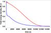 |
Fig. 19 Temporal behaviour of the fast-wave total energy density vs. time in the cooling (red line) and heating (blue line) processes. Total energy density has been normalized with respect to its initial value (kz = 10-6 m-1). |
Finally, it is worth highlighting the presence, in the equations describing the temporal variation of total energy density for slow and fast waves, of the terms describing the temporal variation of the mean atomic weight and of the inverse of the squared sound speed, which appear because of the processes taking place in the plasma. The first term is due to recombination/ionization taking place during the cooling/heating processes while the second appears because of the temperature and mean-atomic-weight time dependence.
10. Conclusions
Until now, all the studies of small-amplitude prominence oscillations have interpreted these oscillations in terms of linear MHD waves. Furthermore, all these studies have been made by exciting small perturbations on a background equilibrium whose physical properties, akin to those of solar prominences, do not change with time (Arregui et al. 2012). However, prominence observations suggest that they are very dynamic plasma structures whose physical properties, such as temperature, density, pressure, and so on, quickly change with time. The first attempt to understand how a temperature increase or decrease modifies the properties of slow waves in a fully ionized prominence-like plasma was made by Ballester et al. (2016). However, prominences are not always fully ionized plasmas, and therefore any increase or decrease of the temperature changes the plasma ionization degree, and these changes also modify the behaviour of plasma microscopic parameters which, at the same time, modify the behaviour of MHD waves. Therefore, here we have made the first attempt to study these effects on MHD waves excited in a hydrogen plasma with physical properties akin to those of prominences. During cooling or heating processes, the ionization degree, and consequently the mean atomic weight, change with time, therefore in the equation describing the specific internal energy, the second term accounting for the ionization potential energy, which depends on the ionization degree, becomes of paramount importance since it has a strong influence on the profile of the temperature’s increase or decrease. However, the effect of this term has sometimes been neglected in studies in which temperature changes due, for instance, to reconnection processes.
First of all, and once an imbalance between radiation and heating has been imposed, in order to mimic cooling/heating processes, we numerically solved the energy equation (see Eq. (26)) suitable for our case, and obtained the time-dependent temperature profiles. From these profiles, we can observe how the ionization or recombination processes taking place affect the temporal behaviour of the temperature. In the heating case, when ionization processes start to take place, the rise of the temperature slows down until the plasma becomes fully ionized. In the cooling case, when recombination processes take place, energy is poured into the plasma and the decrease of the temperature is also slowed down in such a way that it takes quite a long time to reach the final temperature at which the plasma becomes neutral. Once these profiles have been obtained, the temporal behaviour of the different microscopic parameters, such as resistivities, conductivities, electronic, neutral and ion densities, and so on, have also been computed.
Next, we studied the temporal behaviour of Alfvén, slow, and fast waves separately and our conclusions are summarized in the following paragraphs. Alfvén waves propagating parallel to the magnetic field are described by means of Eq. (47), and we observe that its damping is due to the dissipative effect of Cowling’s resistivity. In order to obtain an analytical solution for the perturbed velocity we applied the WKB method and the obtained results have allowed us to make comparisons with the numerical solution. Our results point out important differences with respect to the behaviour of Alfvén waves in a plasma having constant temperature and constant microscopic parameters. When the plasma suffers cooling/heating processes, the temporal variation of resistivities modifies the oscillatory behaviour of Alfvén waves, its period and damping time become time dependent and are no longer constant, the cut-off wavenumbers also become time dependent, and the attenuation rate of the wave is completely different in a cooling or heating process because of the different temporal behaviour of Cowling’s resistivity. These results point out the large number of different situations that can be found in observed prominence oscillations, which correspond to different physical properties as well as to other processes taking place in the plasma. A correct interpretation of the oscillations observed in prominences would be of great importance in order to know with accuracy the physical situation of the prominence plasma under study, that is, to perform prominence seismology.
Slow waves propagating parallel to the magnetic field are described by means of Eq. (66), and their damping is produced by optically thin radiation and by the anisotropic and isotropic thermal conduction of electrons and neutrals, respectively, while resistivities do not play any role. Also, it is worth mentioning the presence in the differential equation of a term describing the temporal variation of the mean atomic weight. We have solved numerically the system of differential equations describing these waves and in order to interpret the obtained results we have computed an approximated expression for the non-adiabatic sound speed and, using this, we have written a dispersion relation for slow waves in a plasma undergoing cooling/heating processes. By numerically solving this dispersion relation, we have obtained the temporal dependence of the period and damping time of slow waves when the plasma is heated or cooled, which has helped us to interpret our numerical results. Again, these results point out that in plasmas suffering heating/cooling processes, wave parameters such as period and damping time display quite different temporal behaviours. For instance, by comparing the behaviour of slow waves in almost neutral or fully ionized plasmas at constant temperature, we have shown how easy it would be to confuse the slow-wave propagation in a cooled plasma with that in an almost fully ionized plasma. Conversely, when the plasma is heated, the period and damping time of slow waves in the heated or in the almost fully ionized plasma are completely different. While in the heated/cooled plasma the period and damping time are time dependent, for the almost fully ionized plasma with constant temperature, these parameters are constant.
Fast waves propagating perpendicular to the magnetic field are described by means of Eq. (74), and we observe that in this case their damping is produced by the joint effect of Cowling’s resistivity and thermal effects, but again it is worth mentioning the presence in the differential equation of the term describing the temporal variation of the mean atomic weight. Although the temporal behaviour of the perturbed velocity corresponding to Alfvén and fast waves is very similar in the cooling case, when the heating case is considered, an important difference appears. While in this case the final attenuation of the Alfvén wave is very weak and takes a long time, for the fast wave, the attenuation is stronger and proceeds more rapidly due to thermal effects. Again, the comparison of the temporal behaviour of the fast-wave perturbed velocity in a heated/cooled plasma with that in an almost neutral plasma with constant temperature, a high value of Cowling’s resistivity and a fixed ionization degree, helps us to understand how the different physical situations influence this behaviour.
Next, for each MHD wave, we analyzed the temporal behaviour of the total energy density. The temporal variation of the total energy density can be written in the form of an equation which on the right-hand-side member includes the sources/sinks of energy. It is instructive to enumerate those terms which, for each wave, always play the role of sinks of energy. In the case of Alfvén waves, the sink term is given by Cowling‘s and Spitzer’s resistivity, however, in the case of slow waves, the sink term corresponds to radiative and conductive losses. For fast waves, the sinks terms are resistivities and thermal losses together. On the other hand, apart from those terms, two other terms appear on the right-hand-side member of the temporal variation of the total energy density for slow and fast waves. These terms come from the temporal variation of the mean atomic weight and sound speed, and, depending on the process considered, they can be sources or sinks of energy. Figures 18 and 19 display the temporal variation of total energy density for slow, Alfvén, and fast waves, and we can observe the good agreement between these plots and the conclusions raised from our analysis of the velocity perturbation corresponding to each wave. For the slow wave, the total energy density decreases more rapidly for the cooling process than for the heating process, which means that attenuation is more efficient in the cooling case, as we found for the velocity perturbation. The same happens for Alfvén and fast waves; the temporal behaviour of total energy densities fully agrees with the temporal behaviour of the velocity perturbations. In particular, if we consider the fast wave and the heating process, we can observe that, after some time, thermal effects dominate and the total energy density decreases towards zero, as we found when the corresponding velocity perturbation was analyzed.
Finally, it is worth mentioning that the obtained periods for the different MHD waves under study satisfy the condition to be greater than the relaxation time by several orders of magnitude, which justifies the use of the single-fluid approximation.
Solar atmospheric seismology aims to determine physical parameters that are difficult to measure by direct means in magnetic and plasma structures. It is a remote diagnostics method that combines observations of oscillations and waves in magnetic structures, together with theoretical results from the analysis of oscillatory properties of given theoretical modes. In the case of prominences (see Arregui et al. 2012), and in order to make meaningful comparisons between observations and theoretical models, it is of key importance to develop, step by step, more complete theoretical models taking into account effects which have not yet been considered. The final aim would be to make available a database of templates of the oscillatory behaviour of the key perturbed variables corresponding to different refined theoretical models. In this sense, this study is a first step to describe the oscillatory behaviour of a partially ionized prominence plasma undergoing heating and cooling processes. Therefore, and from an observational point of view, the described features of perturbed velocities, periods, and damping times obtained from our study are of great interest for the future analysis of prominence oscillation. For instance, in many cases, the usual way to represent the observed damped oscillations is by fitting the time signal with a time-decreasing exponential with a characteristic damping time together with a harmonic function with constant period. Taking into account our results, this fit could lead to incorrect conclusions, since in the case of Alfvén or fast waves the damping of the velocity amplitude does not behave as an exponential function, and therefore we would obtain an incorrect estimation of the period and damping time. Regarding slow waves, our results point out that its velocity amplitude behaves quite differently when heating or cooling processes take place, and this behaviour is also different in a plasma with constant temperature, which again points out how important is to properly recognize the observed oscillation in order to perform meaningful seismological studies. However, we could still think of a worse scenario, since due to the intrinsic inhomogeneity of the prominence medium, we could expect to have different physical situations in different prominence locations. For instance, in some prominence regions, temperature could be rising, while in others it is declining, which produces opposed variations of the microscopic plasma parameters, while at the same time, waves can be excited on this dynamic background. Furthermore, another point of interest is the temporal behaviour of other perturbed variables, such as density, temperature, pressure, and so on, which do not behave in the same way as the velocity perturbation. Therefore, while Doppler velocity information would show some temporal behaviour for the velocity perturbation, spectral line parameters such as intensity, line width, and so on, which could be related to pressure or temperature perturbations (Heinzel et al. 2014; Zapiór et al. 2016), could suggest quite a different behaviour for other perturbed variables. Therefore, forward modeling of the spectral line indicators would be necessary to establish the relation between the variation of plasma perturbations and the temporal evolution of spectral line parameters. At the same time, these considerations point out, again, the inherent difficulty in interpreting the prominence oscillations owing to the many different effects that can be involved.
Finally, in this study, several simplifying assumptions have been considered: among others, we have assumed a constant density; local thermodynamic equilibrium in order to use a Saha equation; and hydrogen plasma. Furthermore, and for the sake of simplicity, a structureless medium has also been considered. Future developments of this research could be to consider a multi-species plasma, which would mean that we would have, simultaneously, a mixture of ionized and neutral species because of the different ionization potentials; at 9000 K, for example, helium is still neutral. Another extension could be to consider a structured medium such as, for example, a cylindrical filament thread, although we would expect that, in spite of the change of geometry, the physical conclusions about the temporal behaviour of MHD waves obtained in this study would remain.
Acknowledgments
The authors acknowledge the support received from MINECO under grant AYA2014-54485-P and FEDER funds. R.S. acknowledges the “Ministerio de Economía, Industria y Competitividad” and the “Conselleria d’Innovació, Recerca i Turisme del Govern Balear (Pla de ciència, tecnologia, innovació i emprenedoria 2013–2017” for the Ramón y Cajal grant RYC-2014-14970. J.T. acknowledges support from MINECO and UIB through a “Ramón y Cajal” grant (RYC-2010-06991). The authors are also grateful to The Leverhulme Trust for funding under grant IN-2014-016.
References
- Anan, T., Ichimoto, K., & Hillier, A. 2017, A&A, 601, A103 [NASA ADS] [CrossRef] [EDP Sciences] [Google Scholar]
- Arregui, I., Oliver, R., & Ballester, J. L. 2012, Liv. Rev. Sol. Phys., 9, 2 [Google Scholar]
- Ballester, J. L. 2015, in Solar Prominences, eds. J.-C. Vial, & O. Engvold, Astrophys. Space Sci. Lib., 415, 259 [Google Scholar]
- Ballester, J. L., Carbonell, M., Soler, R., & Terradas, J. 2016, A&A, 591, A109 [NASA ADS] [CrossRef] [EDP Sciences] [Google Scholar]
- Bender, C. M., & Orszag, S. A. 1978, Advanced Mathematical Methods for Scientists and Engineers [Google Scholar]
- Berger, T. E., Shine, R. A., Slater, G. L., et al. 2008, ApJ, 676, L89 [Google Scholar]
- Braginskii, S. I. 1965, Rev. Plasma Phys., 1, 205 [Google Scholar]
- Carbonell, M., Oliver, R., & Ballester, J. L. 2004, A&A, 415, 739 [NASA ADS] [CrossRef] [EDP Sciences] [Google Scholar]
- Carbonell, M., Oliver, R., & Ballester, J. L. 2009, New Astron., 14, 277 [NASA ADS] [CrossRef] [Google Scholar]
- Field, G. B. 1965, ApJ, 142, 531 [NASA ADS] [CrossRef] [Google Scholar]
- Forteza, P., Oliver, R., Ballester, J. L., & Khodachenko, M. L. 2007, A&A, 461, 731 [NASA ADS] [CrossRef] [EDP Sciences] [Google Scholar]
- Forteza, P., Oliver, R., & Ballester, J. L. 2008, A&A, 492, 223 [NASA ADS] [CrossRef] [EDP Sciences] [Google Scholar]
- Goedbloed, J. P. H., & Poedts, S. 2004, Principles of Magnetohydrodynamics (Cambridge: Cambridge University Press) [Google Scholar]
- Hansen, C. J., Kawaler, S. D., & Trimble, V. 2004, Stellar interiors : physical principles, structure, and evolution (New York: Springer-Verlag) [Google Scholar]
- Heinzel, P., Zapiór, M., Oliver, R., & Ballester, J. L. 2014, A&A, 562, A103 [NASA ADS] [CrossRef] [EDP Sciences] [Google Scholar]
- Hildner, E. 1974, Sol. Phys., 35, 123 [NASA ADS] [CrossRef] [Google Scholar]
- Khomenko, E., Collados, M., & Díaz, A. J. 2016, ApJ, 823, 132 [NASA ADS] [CrossRef] [Google Scholar]
- Leake, J. E., & Arber, T. D. 2006, A&A, 450, 805 [NASA ADS] [CrossRef] [EDP Sciences] [Google Scholar]
- Malherbe, J.-M. 1989, in Dynamics and Structure of Quiescent Solar Prominences, ed. E. R. Priest, Astrophys. Space Sci. Lib., 150, 115 [Google Scholar]
- Malherbe, J. M., & Forbes, T. G. 1986, in NASA Conference Publication, ed. A. I. Poland, 2442 [Google Scholar]
- McAllister, A., Uchida, Y., Tsuneta, S., et al. 1992, PASJ, 44, L205 [NASA ADS] [CrossRef] [Google Scholar]
- Milne, A. M., Priest, E. R., & Roberts, B. 1979, ApJ, 232, 304 [NASA ADS] [CrossRef] [Google Scholar]
- Mouradian, Z., & Soru-Escaut, I. 1989, A&A, 210, 410 [Google Scholar]
- Mouradian, Z., Martres, M. J., & Soru-Escaut, I. 1980, in Japan-France Seminar on Solar Physics, eds. F. Moriyama, & J. C. Henoux, 195 [Google Scholar]
- Mouradian, Z., Martres, M. J., & Soru-Escaut, I. 1986, in NASA Conference Publication, ed. A. I. Poland, 2442 [Google Scholar]
- Mouradian, Z., Soru-Escaut, I., & Pojoga, S. 1995, Sol. Phys., 158, 269 [NASA ADS] [Google Scholar]
- Ofman, L., & Mouradian, Z. 1996, A&A, 308, 631 [Google Scholar]
- Patsourakos, S., & Vial, J.-C. 2002, Sol. Phys., 208, 253 [NASA ADS] [CrossRef] [Google Scholar]
- Prialnik, D. 2000, An Introduction to the Theory of Stellar Structure and Evolution (Cambridge: Cambridge University Press) [Google Scholar]
- Rosner, R., Tucker, W. H., & Vaiana, G. S. 1978, ApJ, 220, 643 [NASA ADS] [CrossRef] [Google Scholar]
- Schmahl, E. J., Mouradian, Z., Martres, M. J., & Soru-Escaut, I. 1982, Sol. Phys., 81, 91 [NASA ADS] [CrossRef] [Google Scholar]
- Soler, R. 2010, Ph.D. Thesis, Departament de Fisica, Universitat de les Illes Balears [Google Scholar]
- Soler, R., Oliver, R., & Ballester, J. L. 2008, ApJ, 684, 725 [NASA ADS] [CrossRef] [Google Scholar]
- Soler, R., Carbonell, M., Ballester, J. L., & Terradas, J. 2013, ApJ, 767, 171 [NASA ADS] [CrossRef] [Google Scholar]
- Soru-Escaut, I., & Mouradian, Z. 1990, A&A, 230, 474 [NASA ADS] [Google Scholar]
- Taliashvili, L., Mouradian, Z., & Páez, J. 2009, Sol. Phys., 258, 277 [NASA ADS] [CrossRef] [Google Scholar]
- Watanabe, T., Kozuka, Y., Ohyama, M., et al. 1992, PASJ, 44, L199 [NASA ADS] [CrossRef] [Google Scholar]
- Zapiór, M., Oliver, R., Ballester, J. L., & Heinzel, P. 2016, ApJ, 827 [Google Scholar]
- Zaqarashvili, T. V., Carbonell, M., Ballester, J. L., & Khodachenko, M. L. 2012, A&A, 544, A143 [NASA ADS] [CrossRef] [EDP Sciences] [Google Scholar]
All Figures
|
Fig. 1 Temperature vs. time for the cooling (red line) and heating (blue line) processes. In all the plots, the initial temperature for the heating process is 4000 K and the final temperature is 9000 K, while in the cooling process, the initial and final temperatures are 9000 K and 4000 K, respectively. Furthermore, from now on, in all the plots optically thin radiation has been considered as well as the same constant density value, ρ = 5 × 10-11 kg m-3. |
| In the text | |
|
Fig. 2 Specific internal energy, e, vs. time for the cooling (left panel) and heating (right panel) processes. Internal energy is represented by red lines, ionization potential energy by blue lines, and both terms together by black lines. |
| In the text | |
|
Fig. 3 Relative density of ions, ξi (left panel) and neutrals, ξn (right panel) vs. time, for cooling (red lines) and heating (blue lines) processes. |
| In the text | |
|
Fig. 4 Logarithms of Spitzer’s resistivity, η (left panel), and of Cowling’s resistivity, ηC (right panel) vs. time, for cooling (red lines) and heating (blue lines) processes. |
| In the text | |
|
Fig. 5 Temporal behaviour of the cut-off wavenumber during cooling (red line) and heating (blue line) processes. |
| In the text | |
|
Fig. 6 Cooling case. Left panel: logarithms of twice the Alfvén speed, 2va, (blue line) and ηCkx (red line) vs. time. Right panel: evanescent behaviour of the Alfvén velocity amplitude (kx = 5 m-1). The velocity amplitude has been normalized. |
| In the text | |
|
Fig. 7 Cooling case. Left panel: logarithms of twice the Alfvén speed, 2va, (blue line) and ηCkx (red line) vs. time. Right panel: real part of the frequency vs. time (kx = 10-6 m-1). |
| In the text | |
|
Fig. 8 Heating case. Left panel: logarithms of twice the Alfvén speed, 2va, (blue line) and ηCkx (red line) vs. time. Right panel: evanescent behaviour of the Alfvén velocity amplitude (kx = 5 × 10⁻⁶ m-1). The velocity amplitude has been normalized. |
| In the text | |
|
Fig. 9 Heating case: real part of the frequency vs. time (kx = 5 × 10⁻⁶ m-1). |
| In the text | |
|
Fig. 10 Comparison of the Alfvén wave velocity amplitude vs. time for the cooling (red line) and heating (blue line) processes. kx = 10-6 m-1. The velocity amplitude has been normalized. |
| In the text | |
|
Fig. 11 Alfvén wave velocity amplitude vs. time. Left panel: plasma cooled from T0(t) = 9000 K to 4000 K (red line); partially ionized plasma with T0 = 5000 K and ξi = 0.02 (blue line). Right panel: plasma heated from T0(t) = 4000 K to 9000 K (red line); partially ionized plasma with T0 = 5000 K and ξi = 0.02 (blue line; kx = 10-6 m-1). The velocity amplitude has been normalized. |
| In the text | |
|
Fig. 12 Temporal behaviour of the logarithm of damping time for the Alfvén wave in the cooling (red line) and heating (blue line) processes (kx = 10-6 m-1). |
| In the text | |
|
Fig. 13 Slow-wave velocity amplitude vs. time. Left panel: plasma cooled from T0(t) = 9000 K to 4000 K (red line); almost fully ionized plasma with T0 = 8000 K and ξi = 0.99 (blue line); almost neutral plasma with T0 = 5000 K and ξi = 0.02 (black line). Right panel: plasma heated from T0(t) = 4000 K to 9000 K (red line); almost fully ionized plasma with T0 = 8000 K and ξi = 0.99 (blue line); almost neutral plasma with T0 = 5000 K and ξi = 0.02 (black line; kx = 10-6 m-1). The velocity amplitude has been normalized. |
| In the text | |
|
Fig. 14 Left panel: slow-wave period vs. time for plasma cooled from T0(t) = 9000 K to 4000 K (red line); almost fully ionized plasma with T0 = 8000 K and ξi = 0.99 (blue line); almost neutral plasma with T0 = 5000 K and ξi = 0.02 (black line). Right panel: slow-wave damping time vs. time for plasma cooled from T0(t) = 9000 K to 4000 K (red line); almost fully ionized plasma with T0 = 8000 K and ξi = 0.99 (blue line); almost neutral plasma with T0 = 5000 K and ξi = 0.02 (black line; kx = 10-6 m-1). |
| In the text | |
|
Fig. 15 Comparison of the slow-wave velocity amplitude vs. time for the cooling (red line) and heating (blue line) processes (kx = 10-6 m-1). The velocity amplitude has been normalized. |
| In the text | |
|
Fig. 16 Comparison of the fast wave velocity amplitude vs. time for the cooling (red line) and heating (blue line) processes (kz = 10-6 m-1). The velocity amplitude has been normalized. |
| In the text | |
|
Fig. 17 Fast wave velocity amplitude vs. time. Left panel: plasma cooled from 9000 K to 4000 K (red line); almost neutral plasma with T = 5000 K and ξi = 0.02 (blue line). Right panel: plasma heated from 4000 K to 9000 K (red line); almost neutral plasma with T = 5000 K and ξi = 0.02 (blue line; kz = 10-6 m-1). The velocity amplitude has been normalized. |
| In the text | |
|
Fig. 18 Left panel: temporal behaviour of the slow-wave total energy density vs. time in the cooling (red line) and heating (blue line) processes. Right panel: temporal behaviour of the Alfvén wave total energy density vs. time in the cooling (red line) and heating (blue line) processes. In both cases, the total energy density has been normalized with respect to its initial value (kx = 10-6 m-1). |
| In the text | |
|
Fig. 19 Temporal behaviour of the fast-wave total energy density vs. time in the cooling (red line) and heating (blue line) processes. Total energy density has been normalized with respect to its initial value (kz = 10-6 m-1). |
| In the text | |
Current usage metrics show cumulative count of Article Views (full-text article views including HTML views, PDF and ePub downloads, according to the available data) and Abstracts Views on Vision4Press platform.
Data correspond to usage on the plateform after 2015. The current usage metrics is available 48-96 hours after online publication and is updated daily on week days.
Initial download of the metrics may take a while.