| Issue |
A&A
Volume 609, January 2018
|
|
|---|---|---|
| Article Number | A90 | |
| Number of page(s) | 12 | |
| Section | Planets and planetary systems | |
| DOI | https://doi.org/10.1051/0004-6361/201731484 | |
| Published online | 18 January 2018 | |
Refraction in exoplanet atmospheres
Photometric signatures, implications for transmission spectroscopy, and search in Kepler data
1 Department of Physics, KTH Royal Institute of Technology, The Oskar Klein Centre, AlbaNova, 106 91 Stockholm, Sweden
e-mail: This email address is being protected from spambots. You need JavaScript enabled to view it.
2 Center for Space and Habitability, University of Bern, Sidlerstrasse 5, 3012 Bern, Switzerland
e-mail: This email address is being protected from spambots. You need JavaScript enabled to view it.
Received: 30 June 2017
Accepted: 27 October 2017
Abstract
Context. Refraction deflects photons that pass through atmospheres, which affects transit light curves. Refraction thus provides an avenue to probe physical properties of exoplanet atmospheres and to constrain the presence of clouds and hazes. In addition, an effective surface can be imposed by refraction, thereby limiting the pressure levels probed by transmission spectroscopy.
Aims. The main objective of the paper is to model the effects of refraction on photometric light curves for realistic planets and to explore the dependencies on atmospheric physical parameters. We also explore under which circumstances transmission spectra are significantly affected by refraction. Finally, we search for refraction signatures in photometric residuals in Kepler data.
Methods. We use the model of Hui & Seager (2002, ApJ, 572, 540) to compute deflection angles and refraction transit light curves, allowing us to explore the parameter space of atmospheric properties. The observational search is performed by stacking large samples of transit light curves from Kepler.
Results. We find that out-of-transit refraction shoulders are the most easily observable features, which can reach peak amplitudes of ~10 parts per million (ppm) for planets around Sun-like stars. More typical amplitudes are a few ppm or less for Jovians and at the sub-ppm level for super-Earths. In-transit, ingress, and egress refraction features are challenging to detect because of the short timescales and degeneracies with other transit model parameters. Interestingly, the signal-to-noise ratio of any refraction residuals for planets orbiting Sun-like hosts are expected to be similar for planets orbiting red dwarfs and ultra-cool stars. We also find that the maximum depth probed by transmission spectroscopy is not limited by refraction for weakly lensing planets, but that the incidence of refraction can vary significantly for strongly lensing planets. We find no signs of refraction features in the stacked Kepler light curves, which is in agreement with our model predictions.
Key words: planets and satellites: atmospheres
© ESO, 2018
1. Introduction
The transit method is one of the most successful at finding exoplanets, with thousands of detections by the Kepler mission (Koch et al. 2010) alone. Transit light curves are typically modelled as planets occulting host stars with non-uniform brightness profiles (Mandel & Agol 2002). Light curves with higher photometric precision reveal additional effects, such as thermal emission from planets (e.g. Charbonneau et al. 2005; Demory et al. 2012) and reflected host star light (e.g. Sudarsky et al. 2000; Demory 2014). Searches for rings and moons have also been carried out (Hippke 2015; Kipping et al. 2015; Heller 2017). Further development of light-curve models is therefore desirable in order to account for physical effects that were previously not included, especially on the verge of the commissioning of new facilities that will significantly improve the current photometric capabilities.
Refraction in exoplanet atmospheres, or “atmospheric lensing”, was first discussed by Seager & Sasselov (2000) and Hubbard et al. (2001), who concluded that refraction is weak at low pressures. Hui & Seager (2002) presented a model and made the first detailed study of the effects of refraction and oblateness on transit light curves. Sidis & Sari (2010) studied refraction in the extreme case of a transparent planet and showed that dips in light curves can be caused by refractive transparent planets. Bétrémieux & Kaltenegger (2015) provide analytic expressions for the column density and deflection angle, and make comparisons with a ray-tracing algorithm. Refraction in exoplanet atmospheres have received increased attention over the past few years and several authors have emphasised that refraction can set the effective planet radius (García Muñoz et al. 2012; Bétrémieux & Kaltenegger 2013, 2014). The implications of the effective surface depth due to refraction on transmission spectroscopy have also been studied (Bétrémieux 2016; Bétrémieux & Swain 2017). Several authors have studied how transmission spectra depend on transit phase and the possibility of using refraction to probe the atmospheric composition at different altitudes (Sidis & Sari 2010; García Muñoz et al. 2012; Misra et al. 2014). Refraction signatures in photometric light curves have been proposed by Misra & Meadows (2014) to serve as an efficient method of identifying clear skies. No attempt has yet been made to detect refraction signals in observational data despite the recent theoretical developments.
This paper studies the effects of refraction on transit light curves and how refraction signals depend on physical properties of exoplanet atmospheres. We compute the expected signal strengths and characteristics for a sample of planets. We then discuss the effects of refraction on planetary transmission spectra. We finally survey the complete Kepler primary mission dataset to search for refraction features.
The paper is organised as follows. We describe the model and suite of test planets in Sect. 2, and present model predictions in Sect. 3. Observations and data reduction are detailed in Sect. 4, and observational results are presented in Sect. 5. We discuss our findings in Sect. 6, and summarise our conclusions in Sect. 7.
2. Model description
We use the following conventions and definitions: residuals are defined as ΔF = FR−FM, where FR is the normalised observed or predicted model flux and FM is the normalised flux of a fitted model. All uncertainties are one standard deviation. We parametrise the stellar surface brightness as I = 1−γ1 (1−ν)− γ2 (1−ν)2, where γ1 and γ2 are the limb-darkening coefficients (LDCs) and  with r as radial distance from the stellar disc centre. The following parameter values are used unless otherwise stated: an impact parameter of 0.5 stellar radii, a photon wavelength of 6500 Å, stellar radius equal to the solar value, γ1 = 0.37, and γ2 = 0.27. The LDCs correspond to the solar values computed using the theoretical tables of Claret & Bloemen (2011) in the Kepler bandpass.
2.1. Refraction model
We present in the following an outline of the atmospheric refraction transit light-curve model of Hui & Seager (2002), to which the reader is referred for a rigorous derivation and comprehensive description of the model. The model assumes isothermal atmosphere in hydrostatic equilibrium and uniform vertical atmospheric composition. We note that a factor of two is missing in Eq. (9) of Hui & Seager (2002), see our Eq. (4). We emphasise that it is the absolute magnitude of the magnification (A) that enters Eq. (1). Negative magnifications signifies that the image has been spatially reversed, but only the photometric amplitude is of interest for refraction light curves. Hui & Seager (2002) also treat the effects caused by oblateness of planets, but in this work planets are assumed to be spherical. In this paper we use the notation shown in Table 1, which is the same as the notation used by Hui & Seager (2002).
List of symbols (Hui & Seager 2002).
Let I(θS−θ∗(t)) be the surface brightness of the star as a function of source position and star-centre position and W(θI) be the occultation kernel of the planet disc, which is 0 when the observed image position is within the planet radius and 1 otherwise. Hui & Seager (2002) verified that the step model was a good approximation to reality. Then, the equations describing atmospheric refraction become ![Mathematical equation: \begin{eqnarray} \label{eq:FF} && F(t) = \int {\rm d}^2\theta_\mathrm{S} \sum_\text{images} |A|\, I(\thetaS - \starangle(t))\, W(\thetaI) \\ \label{eq:AA} && A = \left[ 1 + 2 \psi + \psi^2 + u^2 \tilde\psi(1 + \psi)\right]^{-1} \\ \label{eq:phi} && \psi(u) = - B \sqrt{\frac{\pi H}{2 u D_{\rm OL}}} {\,\rm exp} \Bigg[-\frac{u D_{\rm OL} -R_0}{H}\Bigg] \\ \label{eq:u2phi} && u^2\tilde \psi(u) = B \sqrt{\frac{\pi u D_{\rm OL}}{2H}} \Bigg[1 + \frac{H}{2u D_{\rm OL}} \Bigg] {\,\rm exp} \Bigg[-\frac{u D_{\rm OL} -R_0}{H} \Bigg] \\ \label{eq:uu} && u^2 \equiv ({\theta_\mathrm I^1})^2 + ({\theta_\mathrm I^2})^2 = |\thetaI|^2; \end{eqnarray}](/articles/aa/full_html/2018/01/aa31484-17/aa31484-17-eq35.png) with parameters given by
with parameters given by  and
and  (8)where the approximation DOL ≫ DLS in Eq. (7)holds for exoplanet transits. The transit light curve is given by Eq. (1)and is an integral over the stellar disc, which is treated as a flat surface. The quantities denoted by ψ and
  can be thought of as lensing potentials. The parameter B is essentially just a deflection angle that has been scaled by a ratio of distances and C is the ratio of binding energy to thermal energy.
Physical, atmospheric, and orbital parameters for the test planets.
Much of the physics is captured by the important parameters B and C. Of particular importance is the dividing line between strong and weak lensing  (9)where the system is strongly lensing if the condition is fulfilled (Hui & Seager 2002). Strong lensing occurs when caustics are present. Caustics are source positions for which the magnification diverges (Hui & Seager 2002). A more intuitive and equivalent condition for strong lensing is when photons can be refracted into view by the far side of the planet. The far side is where the image is closer to the planet centre than its source position. A consequence of strong lensing is that the flux can increase above the baseline before and after transit. The baseline refers to the out-of-transit flux. The increase of flux just outside of transit will henceforth be referred to as “refraction shoulders”. Importantly, the information contained in the B and C parameters does not capture all the properties that could be connected to the photometric signal strength. Importantly, refraction can obscure atmospheric layers only if the planet is strongly lensing, which is crucial for transmission spectroscopy (see Sect. 6.2).
Other models for refraction have been published based on a ray-tracing approach (García Muñoz et al. 2012; Bétrémieux & Kaltenegger 2013, 2015; Misra et al. 2014), which implies that the equivalent to the analytic expression for the magnification in Eq. (2)needs to be determined numerically. This approach is computationally more demanding than the model of Hui & Seager (2002), which only requires Eq. (1)to be computed numerically. This is because the assumption of an atmosphere that is isothermal in hydrostatic equilibrium and with uniform vertical composition allows the use of an analytic expression in Eq. (2). We note that Misra & Meadows (2014) reported that the assumption of an isothermal atmosphere results in no significant difference after testing realistic tropospheric lapse rates and stratospheric temperature inversions using their ray-tracing framework. Alternately, Sidis & Sari (2010) developed a model that provides analytic approximations for the observed flux near and away from occultation, but at the cost of ignoring limb darkening.
2.2. Test planets
We construct a suite of test planets for the analysis of refraction transit light curves. Each planet is defined by a set of parameters, T, MP, R0, DLS, and atmospheric composition, where MP is the planet mass and the remaining variables are defined following Hui & Seager (2002, Table 1). The atmospheric composition is related to α by Cauchy’s equation (Appendix A). Let P be the orbital period, G the gravitational constant, MS the stellar mass, σR the cross section for Rayleigh scattering, and assume the planetary orbits to be circular. The remaining parameters needed to compute refraction light curves are then given by (Hui & Seager 2002)  along with Eqs. (1)–(7). Equation (13)assumes that the effective surface is set by Rayleigh scattering. This is a reasonable assumption at a wavelength of 6500 Å in atmospheres devoid of clouds and hazes, which is what is assumed here unless otherwise stated. Importantly, the model is insensitive to the opacity source. The model is constructed such that the optical depth above R0 is zero and infinite below. So, it is perfectly legitimate to ignore the Rayleigh scattering modelled by Eq. (13)and to set ρ0 and R0 manually. For example, if there are reasons to believe that a cloud deck obscures all paths below R0, then R0 can be set to the radius that corresponds to the altitude at the top of the cloud layer, in which case ρ0 would be the atmospheric mass density at R0.
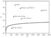 |
Fig. 1 Positions of the test planets presented in Table 2. The black line is the limit between weak and strong lensing; the region above the line is strongly lensing. |
We provide the properties of all test planets in Table 2, while their distribution in the BC-plane is shown in Fig. 1. Earth and Jupiter are used as references for the other fiducial planets. The temperatures for Earth and Jupiter are chosen to be representative of the majority of the atmosphere above the effective Rayleigh surface. A temperature of 255 K is deemed representative of the atmosphere of the Earth and the temperature of 150 K for Jupiter is based on the temperature profile measured by the Galileo atmospheric probe (Seiff et al. 1998, Fig. 28). The temperature of the 80-day super-Earth is assumed to scale as  with respect to the Earth and the temperatures of the 20-day Jovian and 1-year Jovian with respect to Jupiter. The bulk density for the fiducial super-Earth scenario is chosen based on the empirical relation of Weiss & Marcy (2014, Eq. (3)), which is fitted to planets with radii in the range 1.5−4 R⊕. This relation results in a mass of 3.9 M⊕ for a radius of 1.5 R⊕, corresponding to a mean density of 6.4 g cm-3. It is also assumed that the mass distributions within all planets are homogeneous. The average density of the Jovian planets is assumed to be equal to that of Jupiter.
The purpose of the best-case planet is to put a limit on the maximum possible refraction strength. We fix the orbital distance to the orbital distance of Jupiter because it sets the geometrical deflection angle and is of little importance as long as the angle is small (Sect. 3.2). The radius is set to the Jupiter radius because an arbitrarily large signal strength can be achieved by increasing the radius with an appropriate rescaling of the other parameters. This leaves the atmospheric composition, which is set to pure H2; planet mass, which is set to 1 MJ; and the temperature, which is set to 600 K. It is shown in Sect. 3.2 that the atmospheric composition, planet mass, and temperature are degenerate. For example, a doubling in mass and temperature results in an identical light curve to that of the original parameters. The purpose of the best-case planet is that any planet at an orbital distance and with a radius equivalent to those of Jupiter yields a weaker refraction signal. In this sense, the best-case planet scenario can be considered as an upper limit. We note that the Earth happens to show a stronger refraction signal for an Earth-sized planet on a 1-year orbit and can serve as a best-case terrestrial planet.
3. Model predictions
3.1. Refraction light curves
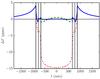 |
Fig. 2 Residuals for a light-curve model including refraction fitted with a plain transit model without refraction for Jupiter. The dash-dotted red line is for a plain model with identical parameters as for the refraction light curve. The dashed green line is for a plain model with fixed, correct limb-darkening coefficients (LDCs). The solid blue line is a plain model fitted with 10% freedom in the LDCs. The vertical black lines mark when the planet limb and centre cross the star limb. The reference time is set to mid-transit. |
The primary question is what differences are caused by atmospheric refraction in transit light curves. This can be studied by generating a light curve using the refraction model of Hui & Seager (2002) and then fitting a model without refraction to it. Residuals (ΔF) can then be computed by taking the refraction light curve and subtracting the fitted model from it. Mathematically, ΔF = FR−FM, where FR is the normalised predicted model flux and FM is the normalised flux of a fitted model. Figure 2 shows residuals for a refraction light curve fitted with plain transit light-curve models without refraction for Jupiter. The fitted models are a plain transit light curve with the parameters fixed to those used for generating the refraction light curve (dash-dotted red); with free inclination, orbital distance, and planet radius but fixed LDCs (dashed green); and with free parameters and 10% freedom in the LDCs (solid blue). The effects of refraction are clearly seen as shoulders before and after transit and a flux decrease appears during transit. The shoulders only exist for planets in the strong lensing regime. The near side of a strongly lensing planet can occult the star before light starts being lensed into view by the far side of the planet, in which case the shoulders are suppressed. This is only relevant for systems close to the limit between strong and weak lensing. Most systems in the strong lensing regime will exhibit shoulders. The flux decrease of ~15 parts per million (ppm; dash-dotted red) at mid-transit for Jupiter is relatively large. For comparison, the corresponding flux decrease for the 1-year Jovian case is ≲ 1 ppm. One of the main points of Fig. 2 is to show that many of the in-transit refraction features are eliminated when fitting a model with free impact parameter, planet radius, and star-planet distance (dashed green), especially when also allowing for some freedom in the LDCs (solid blue).
3.2. Refraction shoulders
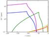 |
Fig. 3 Refraction shoulders for the five strongly lensing test planets. The y-axis is logarithmic for visual clarity. Blue is the reference Jupiter and is identical to the blue line in Fig. 2. Red is the Earth, yellow is the 80-day super-Earth, green is the 80-day Jovian, and magenta is the best-case Jovian planet. The reference time is set to when the planet centre crosses the star limb, which is equivalent to the second vertical line in Fig. 2. |
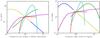 |
Fig. 4 Refraction signal strengths as functions of six different refraction parameters. The left panel is the 80-day super-Earth and the right panel is Jupiter. The x-axis is the ratio of the changing parameter to its original value. Red is wavelength, green is temperature, blue is planet mass, cyan is radius, magenta is orbital distance, and yellow is molecular weight (which overlaps with planet mass). The signal is measured over 60 min for the 80-day super-Earth and 600 min for Jupiter because of the different characteristic timescales. |
Refraction shoulders are expected to be the most easily detectable features and depend on several atmospheric parameters. Figure 3 shows refraction shoulders for the suite of test planets provided in Table 2, except for the 20-day Jovian, which does not exhibit shoulders as it is weakly lensing. The peak residual amplitudes and half-times for the planets are provided in Table 3. A half-time is defined as the time interval measured from when the residual amplitude is half of the peak amplitude to the time when the residual amplitude is at its peak.
Refraction shoulder properties.
Systems with higher peak amplitudes are not necessarily easier to detect. For instance, when comparing the 80-day super-Earth with the Earth, the super-Earth’s refraction shoulders have a higher peak amplitude, but fade over shorter timescales than the shoulders of the Earth.
We explore the parameter space by studying the strength of refraction as a function of the following parameters: observing wavelength, temperature, mass, radius, orbital distance, and molecular weight. This is done by scaling each parameter with respect to the reference value that is provided in Table 2. The molecular weight is scaled by simply assuming that the mass of the atoms that constitute the atmosphere is changing. This means that the refractive properties, which are unique for each molecule, are assumed to be constant. Each parameter is assumed to be independent of the other parameters that are used to define a test planet, but propagates into the quantities that are calculated using the scaled parameter, following the description in Sect. 2.2. For example, the mass is assumed to be constant when the radius is doubled, whereas a parameter such as the surface gravity would be reduced by a factor of 4 following Eq. (11). We thus define the refraction signal strength SΔt as the mean ΔF over the Δt minutes just before first contact. This serves as a measure of the shoulders’ detectability.
Refraction signal amplitudes for various ranges of parameters are shown in Fig. 4. The very steep refraction strength drop-off at shorter wavelengths is primarily explained by the fourth-order wavelength dependence of Rayleigh scattering (see Eq. (12)). The radius R0 is set to the radius at which the optical depth due to Rayleigh scattering is unity. A quickly increasing scattering cross section at shorter wavelengths implies that the effective radius is shifted to higher altitudes where the density is lower. A secondary effect of decreasing wavelength is that the refractive coefficient increases, but this effect is orders of magnitude weaker than that of the increased Rayleigh cross section. The wavelength dependence flattens for long wavelengths because it only determines the capability of the atmosphere to deflect light. This enters the model through the B parameter, which is a deflection angle scaled by distance. Further increased deflection strength beyond the point where the planet is capable of deflecting light from its host star into the line of sight does not result in a significantly stronger signal because the limiting factor becomes the projected area of the atmosphere. This means that B is effectively saturated.
Figure 4 also shows that the refraction signal strength monotonically increases with increasing orbital distance. The signal strength increases more steeply for shorter distances, then reaches a break and keeps increasing more slowly. The steep region is where the refraction strength is limited by the capability of the atmosphere to deflect the light at a large enough angle. The break is the distance at which the B parameter effectively saturates, analogously to the break that is seen in the wavelength dependence. The reason for a continued, slower refraction strength increase for large distances is that the transit timescale lengthens as a consequence of the Keplerian orbits of the planets.
The refraction signal strength has a non-monotonous dependence on some of the parameters. The signal shows the same behaviour with respect to the molecular weight, mass, and inverse temperature because these three parameters enter the equations through B and C identically. The parameters decrease the scale height and increases the density ρ0, both of which result in a larger density gradient of the atmosphere, which increases the atmosphere’s capability of deflecting light. A competing effect is that a decreased scale height also gives a smaller projected atmospheric area, which results in a lower refraction signal. The balance between these two effects yields a parameter value for which the refraction strength is maximised. The density has a stronger dependence on molecular weight than the planet mass and inverse temperature, but this effect is cancelled by a corresponding decrease in the refractive coefficient α.
The strongest dependence of refraction amplitude is on the planet-to-star radius ratio. The refraction signal scales with planet radius because of the increased projected atmospheric area. Additional effects are that the scale height increases and atmospheric density decreases, which at a given radius renders the atmosphere unable to deflect light at large enough angles to be strongly lensing, resulting in a sharp cut-off. It is also possible that the radius is large enough for the near side of the planet to start occulting the star before the far side of the planet starts refracting light into view. In this case, the strength of the refraction signal also drops sharply.
3.3. Red dwarf host star
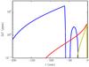 |
Fig. 5 Same as Fig. 3, but with an M4V red dwarf host star. The 1-year Jovian and best-case planet are excluded; they have no shoulders because they fall outside of the strong lensing regime. |
Refraction signal strength is dependent on host star properties, which is investigated by computing the refraction wings for the same test suite of planets but with a red dwarf host. The host star used is a fiducial M4V dwarf star with a radius of 0.26, mass of 0.2, and luminosity of 0.0055 relative to the Sun (Reid & Hawley 2005; Kaltenegger & Traub 2009). The LDCs are set to γ1 = 0.2 and γ2 = 0.4 corresponding to the redder wavelengths of Berta-Thompson et al. (2015) because the flux of a red dwarf is assumed to be weighted towards longer wavelengths in the Kepler bandpass. The test planets are moved to an orbit at which they receive the same incident flux as for a Sun-like host. Only Earth, the 80-day super-Earth, and Jupiter out of the five test planets are in the strongly lensing regime with the M4V dwarf host. The refraction shoulders are shown in Fig. 5. The two most striking differences are that the amplitudes increase by a factor of ~ 5 and the relevant timescales are much shorter, which is clearly seen in Table 3.
We can then compare the detectability of refraction features for Jupiter around the Sun and a Jupiter analogue around an M4V dwarf star. Let ξ be the timescale, L host star luminosity, and assume that the achievable photometric precision (σP) scales as the square root of photon count. The precision is the relative uncertainty from photon counting statistics that can be achieved within a given time interval. For this reason a factor of P− 1/2 is introduced because it is assumed that observations are performed whenever a transit occurs. In this case the precision follows  (14)The period around the dwarf star is six months compared to twelve years around the Sun and the refraction timescale is shorter by a factor of 274/43 ≈ 6.4 (from Table 3) around the dwarf star. The ratio of precision around the Sun to precision around an M4V dwarf after twelve years of observations is then
  (15)The signal strength around the Sun is expected to be weaker by roughly the same amount, see Table 3, so the predicted signal-to-noise ratio (S/N) is similar for the Sun and for an M4V dwarf host. Importantly, the M4V S/N would of course decrease if not all transits are observed within the given time interval.
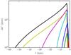 |
Fig. 6 Same as Fig. 3, but for the TRAPPIST-1 system at a wavelength of 4.5 μm corresponding to the infrared Spitzer photometry of Gillon et al. (2017). The planets are TRAPPIST-1b (red), c (green), d (blue), e (cyan), f (magenta), g (yellow), and h (black). |
3.4. TRAPPIST-1
We now focus on the more extreme case of the M8V dwarf TRAPPIST-1, which hosts seven Earth-size planets (Gillon et al. 2017). We compute the refraction shoulders for all TRAPPIST-1 planets at a wavelength of 4.5 μm, corresponding to the infrared Spitzer photometry gathered for this object (Gillon et al. 2017). The nominal effect of limb darkening at 4.5 μm is ignored. It is not reasonable to assume that Rayleigh scattering sets the effective surface at a wavelength of 4.5 μm. Instead, the planet radius (R0) is set to the radius at which the pressure is 1 atm, consequently the mass density ρ0 is set to the density at R0, instead of being computed using Eq. (13). We show the refraction shoulders for all TRAPPIST-1 planets in Fig. 6 and their properties in Table 3. We use the parameters (except for planet masses) from Gillon et al. (2017), an assumed atmospheric composition 0.78N2 + 0.22O2, and planet masses from Wang et al. (2017). The seventh planet, TRAPPIST-1h, shows the strongest refraction signal with a peak excess amplitude of 40 ppm and a half-time of 11 min. It is not reasonable to expect any residual signal to be stronger than 100 ppm for different assumptions concerning the atmospheric composition or when considering the uncertainty of the parameters. This value was determined by exploring the parameter space around TRAPPIST-1h.
The S/N for planets around TRAPPIST-1 and the Sun can be compared using the precision defined by Eq. (14). The luminosity of TRAPPIST-1 is 0.000524 L⊙ and the orbital period of TRAPPIST-1h is 18.8 days (Luger et al. 2017). The distance with an equivalent incident flux around the Sun would correspond to a period of 1677 days. The peak amplitude of the refraction shoulders of a TRAPPIST-1h analogue around the Sun is 1 ppm with a half-time of 73 min. Analogously to Eq. (15), the precision would be higher by a factor of  (16)around the Sun than TRAPPIST-1, which results in a comparable S/N given that the refraction signal is 1 ppm around the Sun compared to 40 ppm around TRAPPIST-1.
3.5. Weak lensing
Any in-transit, ingress, and egress signals are expected to be vanishing for weakly lensing planets because almost all of these refraction effects can be compensated for by fitting a plain transit model, especially when allowing for some freedom in the LDCs. This can be seen for Jupiter in Fig. 2, where the residuals are smaller than 1 ppm between the shoulders when fitting a model with 10% freedom in the LDCs. The 20-day Jovian is a planet that is expected to have relatively strong lensing features even though it is weakly lensing, primarily because it is large and is further away from its host star than the closest close-in giants. Figure 7 shows the residuals for the 20-day Jovian planet along with a set of planets with similar parameters. The main point is that refraction features are not significantly stronger and present on much shorter timescales compared to strongly lensing planets.
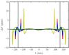 |
Fig. 7 Residuals for a set of 20-day Jovians after fitting a plain light-curve model with 10% freedom in the limb-darkening coefficients to a refraction light curve. Blue is the reference planet with parameters given in Table 2. Red is double temperature, green is double mass, cyan is six times higher molecular weight, and yellow is double radius. The vertical black lines mark when the planet centre crosses the star limb. The reference time is set to mid-transit. |
4. Observations
We then turn to observations where transit light curves from Kepler are stacked and fitted in an attempt to detect refraction features. Kepler 30-min long-cadence simple aperture photometry (SAP) Jenkins et al. (2010, data release 25) are used for the analysis. The products in the SAP data used for our purpose are the timestamps, photometric fluxes, 1-σ statistical flux errors, and quality flags. Data for all Kepler objects of interest (KOIs) from quarters 0 through 17 were downloaded from NASA Exoplanet Archive1 (NEA) on 23 January 2017. The SAP data have Argabrightening events mitigated (Witteborn et al. 2011) and cosmic rays removed. Background estimates are then subtracted and the photometric fluxes are computed using optimal apertures. The SAP is a less processed version than the pre-search data conditioning SAP (PDCSAP) (Stumpe et al. 2012; Smith et al. 2012), which has undergone additional artefact mitigation to account for instrument systematics. The choice of using SAP instead of PDCSAP is made because the artefacts primarily affect longer timescales and additional high-level data reduction increases the risk of either removing refraction signals or introducing weak systematics that could be confused with refraction-driven patterns in the data. Concerning false positives, Fressin et al. (2013) determined that 90% of all KOIs are real planets.
4.1. Light curve reduction and fitting
The Kepler photometry data are reduced and fitted in order to study any systematic residuals. All transits for each KOI are stacked and only data corresponding to five transit durations centred on the transit are kept for each transit. All data points during transits of other KOIs in the same system or flagged as bad in the SAP are removed. Bad means that the flag SAP_QUALITY is different from 0. This conservative rejection criterion is chosen because systematic residuals were observed otherwise. Each transit is individually normalised by dividing the data with a quadratic polynomial that is fitted to the out-of-transit baselines, which are defined as the first and last 1.5 transit durations out of the five transit durations. This means that the actual transit and half a transit duration before and after the transit are excluded. The additional margin is introduced because of potential refraction shoulders during the time intervals just before and after transit. The transit light-curve model of Mandel & Agol (2002) is then fitted to the stack of all transits for each KOI. Transit timing variations (TTVs) are modelled by introducing a sinusoidal shift in time. Light curve fitting is performed using the Levenberg-Marquardt gradient descent function curve_fit in SciPy 0.13.3 with eight free parameters; star-planet distance, planet radius, inclination, two LDCs and three TTV parameters. The LDCs are given 10% freedom with respect to the values in NEA, which are derived using the method of Claret & Bloemen (2011) using the ATLAS model and least-squares method with effective temperatures and surface gravities from Huber et al. (2014). The three TTV parameters are the amplitude, frequency, and initial phase of the sinusoidal shift in time. A 5-σ clip is then applied to the data meaning that points with a photometric residual of more than five sigma are removed. A second normalisation using the same conservative baseline is then performed with the additional requirement that the normalisation function is fitted to at least five points on each side. A minimum of 14 data points between the baseline intervals are demanded to ensure that the reference level is well determined and that the transit contains a meaningful amount of information. Transits with too few points are removed and the remaining stacked transits are refitted.
The accuracy of the photometric baseline for each transit is checked using two tests (Sheets & Deming 2014). Firstly, a line is fitted to the first interval and projected to the other side of transit. The transit is rejected if the mean of the projection at the time of the other baseline deviates by more than 0.001 (relative flux) from 0. It was verified that the choice of 0.001 resulted in a reasonable balance between number of rejected transits and light-curve quality. The projection is then reversed by fitting to the second interval and projecting to the first. It is possible that a transit light curve passes one but not both parts of the test. Secondly, it is required that the two lines from the projection test have slopes that are consistent with 0 at 3-σ. Only transits with both slopes being consistent with 3-σ are kept for further analysis. Light curve fits are then performed for each KOI to the stack of the transits that passed both tests. Finally, the deviations of the residuals are tested for systematics using the red-noise test presented in Sheets & Deming (2014). If the noise is solely composed of statistical fluctuations, such as for photon counting, then log (σ) ∝ −0.5log (N), where σ is the sample standard deviation and N is the size of the bins. The stacked residuals for all transits of a given KOI are binned with different bin sizes, allowing for fitting of log (σ) against log (N). Only KOIs with fitted noise slopes in the range −0.8 to −0.3 are kept. This is an efficient way to filter KOIs with various systematic errors on different timescales.
A total of 2394 out of the 4707 KOI light curves pass all tests. The median reduced χ2 value for the 2394 fits is 1.24 and the arithmetic mean is 1.47. The distribution of the number of degrees of freedom (d.o.f.) for the 2394 planets has a median of 8680 and arithmetic mean of 13 733. The primary condition that candidates failed was the requirement of 14 data points between the intervals used for baseline fitting. This is essentially equivalent to requiring transits to be longer than three hours, which excludes 1743 KOIs. These are close-in planets and are not expected to show any refraction signal because of the geometry of the planetary system and the refraction timescale compared to the 30-min cadence of Kepler. This scenario is studied in Sect. 3.5; examples are shown in Fig. 7.
4.2. Selection of candidates
A subset of 305 out of the 2394 fitted KOIs are selected based on the following criteria. It is required that the planet radius is larger than 0.025 stellar radii and orbital period longer than 40 days. This is based on theoretical expectations of which planet population would show the strongest refraction signals. The choice of having an orbital-period requirement instead of star-planet distance cut-off is because the period is more robust as it is measured directly in contrast to the star-planet distance, which is determined by the multi-dimensional light-curve fit. It is required that fitted planet radii should be smaller than 0.5 of the host star radius and that impact parameters be smaller than 1. These criteria mainly reject poorly fitted KOIs. The subset of 305 large planets with long orbits will henceforth serve as the primary sample in the analysis. The median reduced χ2 value for the 305 selected planets is 1.22 and the arithmetic mean is 1.46. The distribution of the d.o.f. for the 305 planets has a median of 3358 and arithmetic mean of 3941.
5. Stacked Kepler data
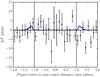 |
Fig. 8 Binned residuals for the sample of 305 large planets on long orbits. The blue line is the theoretical prediction for a Jovian planet on a 1-year orbit. The precision of the stacked residuals is clearly not high enough to detect any refraction signal. Negative distances are before mid-transit and positive distances are after. The vertical black lines mark when the planet centre crosses the star limb. |
Figure 8 shows the stacked residuals for the selected sample of 305 large planets with long orbits. A total of 101 557 long-cadence data points are stacked, with an average of 3174 points per bin. The bins are 0.125 wide in units of host star radii. The relatively long timescale is chosen to reveal refraction shoulders. The residual signal is expected to be of the order of 1 ppm. The precision of the stacked residuals is in the range 2.3–8.4 ppm, implying that any refraction shoulders are not expected to be detectable. The increased noise towards mid-transit occurs primarily because many projected KOI transits do not cross the central parts of the host star, resulting in fewer data points. The blue line is the theoretical prediction for a Jovian planet on a 1-year orbit. It is not a best-case scenario, but a signal in the averaged residuals can most likely not be expected to be stronger than that of a 1-year Jovian. This is determined by exploring the parameter space and studying the residuals for many planets in the sample.
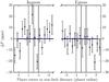 |
Fig. 9 Binned residuals for the sample of large planets on long orbits. Contrary to Fig. 8, the x-axis is the distance from the stellar limb to the planet centre in units of planet radii. The blue line is the theoretical prediction for a Jovian planet on a 20-day orbit. It is equivalent to the blue line in Fig. 4 as observed through the 30-min long cadence of Kepler. Negative distances are when planets are inside of the stellar disc and positive distances are outside. The vertical black lines mark when the planet limb and centre cross the star limb. |
Figure 9 shows the stacked residuals around ingress and egress for the sample of 305 large planets with long orbits. The sample is the same as in Fig. 8, but contrary to Fig. 8, the data in Fig. 9 have the x-axis in units of planet radii. Additionally, the distance on the x-axis is the distance from the stellar limb to the planet centre. A total of 28 911 data points are stacked, with an average of 903 per bin. The choice of unit is made because refraction features around ingress and egress are expected to scale with planet size. This is in contrast with the refraction shoulders that scale with the planet-centre to star-centre distance. Furthermore, each bin is half a planet radius wide allowing for resolution of features on shorter timescales. The purpose of this figure is to reveal any potential features that are similar to those shown in Fig. 7. This would be the only refraction signal for planets that are not strongly lensing. The signal is expected to be a few tenths of ppm at Kepler long cadence and the precision of the stacked residuals is approximately 7 ppm. Thus, any refraction features are not expected to be detectable in this case.
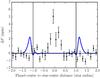 |
Fig. 10 Same as Fig. 8, but for all 2394 KOIs that were fitted. The blue line was computed for a 1-year Jovian and is not representative for the stacked planets. It is not the expected signal for the sample and is included for reference only. |
A blind search for any systematic residuals at a high precision in the sample of all 2394 fitted KOIs is made by stacking the residuals at a bin size of 0.125 star radii, shown in Fig. 10. The stack contains a total of 2.7 million long-cadence data points with an average of 84 thousand per bin. The precision during the transit ranges from 0.3–1 ppm. The residual excess centred on mid-transit possibly stems from inaccurate TTV fitting. The three-parameter TTV model (Sect. 4.1) lowered the reduced χ2 value from 1.481 for 5.34 × 10⁶ d.o.f. to 1.469 for 5.46 × 10⁶ d.o.f. (more d.o.f. with the TTV model because more transits passed all tests). The distributions of reduced χ2 values both with and without TTV modelling are skewed towards large values and have medians of 1.237 and 1.239, respectively. A TTV model with more freedom which allowed each transit to shift slightly in time and another model allowing each transit to shift with respect to the previous one were tested. Both were discarded because they introduced artefacts around ingress and egress. It is clear from Fig. 10 that no systematic residuals are observed out of transit. Any feature at a few ppm, such as signs of rings or moons, would be obvious.
No significant differences to the presented results are observed when dividing the KOIs into other subsets. This includes separating the sample into narrow ranges of star-planet distances and planet sizes. Effects of other fitting parameters and selection criteria are also studied.
6. Discussion
6.1. Connection with physical properties
The refraction strength is very sensitive to the atmospheric scale height, composition, and density, potentially allowing for constraints on the atmosphere using solely photometric data. However, parameters such as the planet radius and orbital distance are more strongly constrained by other observational methods than atmospheric lensing.
Refraction also allows for constraints on the presence of clouds or hazes in the atmosphere. No refraction can be observed in atmospheric layers that are opaque due to clouds, hazes, or other obscuring weather conditions, implying that any refraction features can be taken as an indication of relatively clear skies. Searching for refraction residuals using photometry alone can therefore yield suitable targets for follow-up observations, as previously pointed out by Misra & Meadows (2014). An alternative approach to detect refraction is to measure molecular feature wing steepness and relative depths of absorption features in near-infrared transmission spectra (Benneke & Seager 2013).
Refraction shoulders, which are only possible in the strong lensing regime, are likely to be easier to observe than any ingress, egress, or in-transit residuals. Refraction will be very challenging to detect for weakly lensing systems because the timescales are much shorter. We note that the refraction residuals are usually compensated for when adjusting a transit model to the data. These residuals can also be confused with stellar oscillations, starspots, and other minor effects such as rings and moons (Hippke 2015; Kipping et al. 2015; Heller 2017). An additional source of error is the accuracy of the stellar surface brightness profile. The nature of the refraction shoulders, being out of transit, facilitates the interpretation of the refraction signal.
There is no simple relation between most physical parameters and refraction strength. It is a trade-off that depends on many parameters, as is shown in Sect. 3.2. The only predictor for refraction that is robust is if the system is strongly lensing, but this does not immediately translate to signal strength. The exact position in the BC-plane is not simply correlated with refraction signal strength, although it does give some information on qualitative features (e.g. the overall shape of the refraction residuals), but contains little quantitative information. It is worth emphasising that refraction can set the effective radius only if the planet is strongly lensing, which is important for transmission spectroscopy and is further discussed in Sect. 6.2. The largest refraction peak amplitudes for realistic planets orbiting Sun-like stars are on the order of 10 ppm, see Sect. 3 and Misra & Meadows (2014), but amplitudes as large as 100 ppm have been reported for hypothetical fiducial planets (Hui & Seager 2002; Sidis & Sari 2010). The Earth and the best-case Jovian can be used as examples of planets with high refraction signal strength given their respective orbital distance and radius. The exact signal strength is sensitive to a set of parameters and only seems to be strong for certain combinations, which means that refraction will be an important effect for a small number of planets that happen to be favourable for lensing.
6.2. Effects on transmission spectroscopy
Refraction has attracted much attention as it could increase the effective radius of a planet and set a “surface” above the deepest layers of the atmosphere, which has critical consequences for transmission spectroscopy (García Muñoz et al. 2012; Bétrémieux & Kaltenegger 2013, 2014; Bétrémieux 2016; Bétrémieux & Swain 2017). This effect is more pronounced for in-transit transmission spectra and it was emphasised by Misra et al. (2014) that deeper layers can be probed out of transit in such cases. There is a deep connection between refraction shoulders, which are observed out of transit, and the maximum depth reached by in-transit transmission spectroscopy. The reason the deepest layers are obscured in cases where refraction sets an effective surface is that any light passing through the deep layers are deflected at a large enough angle such that no light from these regions reaches the observer while the planet is in transit. This also means that the light that penetrates deeply into the atmosphere can be observed near transit because of the large deflection angles, which was first pointed out by Sidis & Sari (2010; their Figs. 2 and 3) and then also by Misra et al. (2014; their Fig. 9). The photon paths that pass the deep layers and consequently are deflected at large angles also constitute the refraction shoulders. Combining the above arguments means that weakly lensing planets cannot have an effective surface set by refraction because they are not capable of deflecting light at large enough angles. The scenario is more complicated if the planet is strongly lensing because some parts of the atmosphere become inaccessible during parts of or throughout the transit. It is therefore not necessary for atmospheric layers to be obscured throughout the entire transit, but that the effective exposure time is altitude dependent. Obscured deep layers can be recovered to some extent by observing the out-of-transit spectra in the refraction shoulders. The signal is weaker out of transit because of the geometry that effectively only exposes a narrow slit of the atmosphere on the outer side of the planet to starlight. This means that refraction can have significant effects on transmission spectra for strongly lensing planets even if refraction shoulders cannot be detected because of insufficient photometric precision. In the most extreme cases, the deepest layers may not even be observable out of transit because photons beyond a certain depth are effectively trapped by the atmosphere. This possibility is clearly conceptualised by Sidis & Sari (2010) who discuss the trapping of photons in transparent planets and the idea of a “lower boundary” defined by Bétrémieux & Kaltenegger (2015).
Refraction is only weakly dependent on wavelength and is unlikely to introduce any artefacts that can be interpreted as spectral features in transmission spectra. The wavelength dependence of refraction is incorporated in the model through R0 and the refractive coefficient α (Appendix A). Only the latter is inherent to refraction, whereas the former is a radius set by absorption due to other processes. The inherent wavelength dependence of refraction can be neglected for practically all realistic cases. However, it is possible that refraction becomes significant at wavelengths where the atmosphere is optically thin but very weak close to strong absorption features or towards shorter wavelengths where Rayleigh scattering becomes important. In this case, any effects of refraction will be restricted to the low-opacity regimes. The general guideline is that refraction does not obscure layers of the atmosphere if the planet is weakly lensing. Weak lensing could be restricted to certain wavelengths if the opacity is wavelength dependent or it could be restricted to some transits because of transient clouds or hazes.
6.3. Host star
Refraction features depend on host star parameters. Smaller stars result in larger relative amplitudes for all features because all normalised quantities scale with the ratio of projected planet area to star area. An extreme case of a peak amplitude of 950 ppm was reported by Misra & Meadows (2014) for a 200 K Saturn analogue around an M9V dwarf. The downside is that the luminosity for small dwarf stars is much lower and orbits with the same incident flux as for Sun-like stars are closer-in, which means that the transit duration is shorter but repeats more often. The change in S/N of any refraction signal is much less than the peak amplitude might suggest when all parameters are taken into account, as shown in Sect. 3.3. Misra et al. (2014) and Bétrémieux & Kaltenegger (2014) reported that deeper layers of planet atmospheres can be probed for analogous planets around cooler stars. This means that transmission spectra can contain information from different parts of the atmosphere although the S/N of photometric residuals is expected to be approximately the same for different host stars (Sect. 3.3). It was also shown that only three out of the five strongly lensing planets around Sun-like hosts are strongly lensing if orbiting an M4V dwarf. Going from strongly to weakly lensing shows that deeper layers of atmospheres can be probed around dwarf stars than around Sun-like stars because weakly lensing planets are guaranteed to have their entire atmospheres exposed throughout transits, implying that layers that are inaccessible around a Sun-like star are exposed around red dwarfs.
6.4. Alternative refraction scenarios
It is possible for the atmosphere of an exoplanet to lens a background star, analogously to gravitational microlensing. The refraction model predicts infinite amplification for background lensing, which clearly is an artefact of an idealisation. A more realistic guess would be an amplification of a factor of a few, based on observed gravitational microlensing light curves. The main difficulty becomes the occurrence rate. The cross section is a few AU for gravitational lensing compared to a planet diameter for atmospheric lensing. The brightness increase does not have to be mixed with the host star light if the lensing planet can be directly imaged, since the lensed images of the background star will be in the atmosphere of the exoplanet. Importantly, any lensed light would have been transmitted through the atmosphere, thereby having its spectral imprint.
Another consequence of atmospheric lensing is that it is possible for planets with a near-transiting geometry to increase the flux without ever occulting the host star. This is just the effect of having a system that would have refraction shoulders if it was transiting, but instead showing a single flux excess peak when it passes the star without entering the stellar disc.
6.5. Kepler observations
No refraction signal is observed in the Kepler data when transits are stacked. The achieved precision is not high enough to constrain refraction in the sample of large planets in long orbits, which is the population where refraction is expected to be significant. It is still possible that refraction is relatively strong for a few targets, but these get suppressed when stacked with the rest of the sample. No attempt was made to constrain refraction in individual sources because computing refraction light curves is computationally intensive and the observational precision is clearly lower than predicted refraction shoulder amplitudes.
A lack of refraction signatures in the stack of all fitted planets is expected because the transit method is generally biased towards detecting planets on short orbital periods. The short planet-to-star distance is disadvantageous for refraction because it requires atmospheres to deflect light at larger angles. The only systematic residuals that can be seen in the stack of all planets is the central excess with a peak amplitude of 5 ppm.
7. Conclusions
We have studied the effects of atmospheric refraction on transit light curves and searched for refraction signatures in data from the Kepler mission. Our main conclusions are the following:
-
1.
Refraction residuals in photometric data can constrainphysical properties of exoplanet atmospheres, such as density,scale height, and to some extent composition.
-
2.
Out-of-transit refraction shoulders are the most robust and detectable residuals induced by atmospheric lensing and can reach peak residual excess amplitudes of approximately 10 ppm. More probable amplitudes are a few ppm or less for Jovians and sub-ppm for super-Earths. In-transit, ingress, and egress features are probably very challenging to detect because of short timescales and degeneracy with other transit-model parameters.
-
3.
The parameter space is highly complex and depends critically on a number of the parameters parametrising a planetary system. Refraction will prove important for some targets whereas most planets will show very weak refraction signals.
-
4.
Effects of refraction on transmission spectroscopy are deeply connected with refraction shoulders. Refraction does not set the effective radius if the planet is weakly lensing. The impact of refraction on transmission spectra for strongly lensing planets can vary greatly.
-
5.
The detectability of refraction signals for planets orbiting red dwarfs cannot be assessed by the sole increase in peak residual amplitude. A combination of shorter timescale, shorter orbits, shorter star-planet distance, and host star properties results in similar values of S/N for planets orbiting Sun-like hosts. However, the altitudes probed can be different even though the S/N is approximately the same.
-
6.
Refraction residuals cannot be observed in stacked Kepler light curves because of insufficient photometric precision. The only systematic deviation across the entire Kepler sample is a central excess of a few ppm.
While the present paper was in review, we learnt of a similar study by Dalba (2017). It also explores the dependence of peak
residual excess amplitude on atmospheric parameters and shows comparable results.
Acknowledgments
We thank the anonymous referee for the helpful comments that improved the manuscript. B.-O.D. acknowledges support from the Swiss National Science Foundation in the form of a SNSF Professorship (PP00P2-163967). This paper includes data collected by the Kepler mission. Funding for the Kepler mission is provided by the NASA Science Mission directorate. This research has made use of the NASA Exoplanet Archive, which is operated by the California Institute of Technology, under contract with the National Aeronautics and Space Administration under the Exoplanet Exploration Program. This research made use of Astropy, a community-developed core Python package for Astronomy (Astropy Collaboration et al. 2013). This research has made use of NASA’s Astrophysics Data System Bibliographic Services.
References
- Astropy Collaboration, Robitaille, T. P., Tollerud, E. J., et al. 2013, A&A, 558, A33 [NASA ADS] [CrossRef] [EDP Sciences] [Google Scholar]
- Benneke, B., & Seager, S. 2013, ApJ, 778, 153 [NASA ADS] [CrossRef] [Google Scholar]
- Berta-Thompson, Z. K., Irwin, J., Charbonneau, D., et al. 2015, Nature, 527, 204 [NASA ADS] [CrossRef] [PubMed] [Google Scholar]
- Bétrémieux, Y. 2016, MNRAS, 456, 4051 [NASA ADS] [CrossRef] [Google Scholar]
- Bétrémieux, Y., & Kaltenegger, L. 2013, ApJ, 772, L31 [NASA ADS] [CrossRef] [Google Scholar]
- Bétrémieux, Y., & Kaltenegger, L. 2014, ApJ, 791, 7 [NASA ADS] [CrossRef] [Google Scholar]
- Bétrémieux, Y., & Kaltenegger, L. 2015, MNRAS, 451, 1268 [CrossRef] [Google Scholar]
- Bétrémieux, Y., & Swain, M. R. 2017, MNRAS, 467, 2834 [NASA ADS] [CrossRef] [Google Scholar]
- Born, M., & Wolf, E. 1999, Principles of optics: electromagnetic theory of propagation, interference and diffraction of light (Cambridge University Press) [Google Scholar]
- Charbonneau, D., Allen, L. E., Megeath, S. T., et al. 2005, ApJ, 626, 523 [NASA ADS] [CrossRef] [Google Scholar]
- Claret, A., & Bloemen, S. 2011, A&A, 529, A75 [NASA ADS] [CrossRef] [EDP Sciences] [Google Scholar]
- Dalba, P. A. 2017, ApJ, 848, 91 [NASA ADS] [CrossRef] [Google Scholar]
- Demory, B.-O. 2014, ApJ, 789, L20 [NASA ADS] [CrossRef] [Google Scholar]
- Demory, B.-O., Gillon, M., Seager, S., et al. 2012, ApJ, 751, L28 [Google Scholar]
- Fressin, F., Torres, G., Charbonneau, D., et al. 2013, ApJ, 766, 81 [NASA ADS] [CrossRef] [Google Scholar]
- García Muñoz, A., Zapatero Osorio, M. R., Barrena, R., et al. 2012, ApJ, 755, 103 [NASA ADS] [CrossRef] [Google Scholar]
- Gillon, M., Triaud, A. H. M. J., Demory, B.-O., et al. 2017, Nature, 542, 456 [NASA ADS] [CrossRef] [PubMed] [Google Scholar]
- Griffiths, D. 1999, Introduction to Electrodynamics (Prentice Hall) [Google Scholar]
- Heller, R. 2017, ArXiv e-prints [arXiv:1701.04706] [Google Scholar]
- Hippke, M. 2015, ApJ, 806, 51 [NASA ADS] [CrossRef] [Google Scholar]
- Hubbard, W. B., Fortney, J. J., Lunine, J. I., et al. 2001, ApJ, 560, 413 [NASA ADS] [CrossRef] [Google Scholar]
- Huber, D., Silva Aguirre, V., Matthews, J. M., et al. 2014, ApJS, 211, 2 [NASA ADS] [CrossRef] [Google Scholar]
- Hui, L., & Seager, S. 2002, ApJ, 572, 540 [NASA ADS] [CrossRef] [Google Scholar]
- Jenkins, J. M., Caldwell, D. A., Chandrasekaran, H., et al. 2010, ApJ, 713, L120 [NASA ADS] [CrossRef] [Google Scholar]
- Kaltenegger, L., & Traub, W. A. 2009, ApJ, 698, 519 [NASA ADS] [CrossRef] [Google Scholar]
- Kipping, D. M., Schmitt, A. R., Huang, X., et al. 2015, ApJ, 813, 14 [NASA ADS] [CrossRef] [Google Scholar]
- Koch, D. G., Borucki, W. J., Basri, G., et al. 2010, ApJ, 713, L79 [NASA ADS] [CrossRef] [Google Scholar]
- Luger, R., Sestovic, M., Kruse, E., et al. 2017, Nature Astron., 1, 0129 [Google Scholar]
- Mandel, K., & Agol, E. 2002, ApJ, 580, L171 [NASA ADS] [CrossRef] [Google Scholar]
- Misra, A. K., & Meadows, V. S. 2014, ApJ, 795, L14 [CrossRef] [Google Scholar]
- Misra, A., Meadows, V., & Crisp, D. 2014, ApJ, 792, 61 [CrossRef] [Google Scholar]
- Reid, I. N., & Hawley, S. L. 2005, New light on dark stars: red dwarfs, low-mass stars, brown dwarfs (Praxis Publishing Ltd.) [Google Scholar]
- Seager, S., & Sasselov, D. D. 2000, ApJ, 537, 916 [NASA ADS] [CrossRef] [Google Scholar]
- Seiff, A., Kirk, D. B., Knight, T. C. D., et al. 1998, J. Geophys. Res., 103, 22857 [NASA ADS] [CrossRef] [Google Scholar]
- Sheets, H. A., & Deming, D. 2014, ApJ, 794, 133 [NASA ADS] [CrossRef] [Google Scholar]
- Sidis, O., & Sari, R. 2010, ApJ, 720, 904 [NASA ADS] [CrossRef] [Google Scholar]
- Smith, J. C., Stumpe, M. C., Van Cleve, J. E., et al. 2012, PASP, 124, 1000 [NASA ADS] [CrossRef] [Google Scholar]
- Stumpe, M. C., Smith, J. C., Van Cleve, J. E., et al. 2012, PASP, 124, 985 [NASA ADS] [CrossRef] [Google Scholar]
- Sudarsky, D., Burrows, A., & Pinto, P. 2000, ApJ, 538, 885 [NASA ADS] [CrossRef] [Google Scholar]
- Wang, S., Wu, D.-H., Barclay, T., & Laughlin, G. P. 2017, ApJ, submitted [arXiv:1704.04290] [Google Scholar]
- Weiss, L. M., & Marcy, G. W. 2014, ApJ, 783, L6 [NASA ADS] [CrossRef] [Google Scholar]
- Witteborn, F. C., Van Cleve, J., Borucki, W., Argabright, V., & Hascall, P. 2011, in Techniques and Instrumentation for Detection of Exoplanets V, Proc. SPIE, 8151, 815117 [CrossRef] [Google Scholar]
Appendix A: Cauchy’s equation
Cauchy’s equation is used to compute the refractive coefficient (α) for different atmospheric compositions. The refractive coefficient is not to be confused with the refractive index (n), which are related by n = 1 + αρ, where ρ is the density. The refractive coefficient is given by αρ = A1(1 + B1/λ2), where A1 is the coefficient of refraction, B1 is the coefficient of dispersion, and λ is the wavelength. Coefficients for some common gases are provided in Table A.1. The refractive coefficients are calculated at a temperature of 0 °C and pressure of 1 atm, and are assumed to be constant over the relevant temperatures and pressures.
Cauchy’s equation coefficients.
All Tables
All Figures
|
Fig. 1 Positions of the test planets presented in Table 2. The black line is the limit between weak and strong lensing; the region above the line is strongly lensing. |
| In the text | |
|
Fig. 2 Residuals for a light-curve model including refraction fitted with a plain transit model without refraction for Jupiter. The dash-dotted red line is for a plain model with identical parameters as for the refraction light curve. The dashed green line is for a plain model with fixed, correct limb-darkening coefficients (LDCs). The solid blue line is a plain model fitted with 10% freedom in the LDCs. The vertical black lines mark when the planet limb and centre cross the star limb. The reference time is set to mid-transit. |
| In the text | |
|
Fig. 3 Refraction shoulders for the five strongly lensing test planets. The y-axis is logarithmic for visual clarity. Blue is the reference Jupiter and is identical to the blue line in Fig. 2. Red is the Earth, yellow is the 80-day super-Earth, green is the 80-day Jovian, and magenta is the best-case Jovian planet. The reference time is set to when the planet centre crosses the star limb, which is equivalent to the second vertical line in Fig. 2. |
| In the text | |
|
Fig. 4 Refraction signal strengths as functions of six different refraction parameters. The left panel is the 80-day super-Earth and the right panel is Jupiter. The x-axis is the ratio of the changing parameter to its original value. Red is wavelength, green is temperature, blue is planet mass, cyan is radius, magenta is orbital distance, and yellow is molecular weight (which overlaps with planet mass). The signal is measured over 60 min for the 80-day super-Earth and 600 min for Jupiter because of the different characteristic timescales. |
| In the text | |
|
Fig. 5 Same as Fig. 3, but with an M4V red dwarf host star. The 1-year Jovian and best-case planet are excluded; they have no shoulders because they fall outside of the strong lensing regime. |
| In the text | |
|
Fig. 6 Same as Fig. 3, but for the TRAPPIST-1 system at a wavelength of 4.5 μm corresponding to the infrared Spitzer photometry of Gillon et al. (2017). The planets are TRAPPIST-1b (red), c (green), d (blue), e (cyan), f (magenta), g (yellow), and h (black). |
| In the text | |
|
Fig. 7 Residuals for a set of 20-day Jovians after fitting a plain light-curve model with 10% freedom in the limb-darkening coefficients to a refraction light curve. Blue is the reference planet with parameters given in Table 2. Red is double temperature, green is double mass, cyan is six times higher molecular weight, and yellow is double radius. The vertical black lines mark when the planet centre crosses the star limb. The reference time is set to mid-transit. |
| In the text | |
|
Fig. 8 Binned residuals for the sample of 305 large planets on long orbits. The blue line is the theoretical prediction for a Jovian planet on a 1-year orbit. The precision of the stacked residuals is clearly not high enough to detect any refraction signal. Negative distances are before mid-transit and positive distances are after. The vertical black lines mark when the planet centre crosses the star limb. |
| In the text | |
|
Fig. 9 Binned residuals for the sample of large planets on long orbits. Contrary to Fig. 8, the x-axis is the distance from the stellar limb to the planet centre in units of planet radii. The blue line is the theoretical prediction for a Jovian planet on a 20-day orbit. It is equivalent to the blue line in Fig. 4 as observed through the 30-min long cadence of Kepler. Negative distances are when planets are inside of the stellar disc and positive distances are outside. The vertical black lines mark when the planet limb and centre cross the star limb. |
| In the text | |
|
Fig. 10 Same as Fig. 8, but for all 2394 KOIs that were fitted. The blue line was computed for a 1-year Jovian and is not representative for the stacked planets. It is not the expected signal for the sample and is included for reference only. |
| In the text | |
Current usage metrics show cumulative count of Article Views (full-text article views including HTML views, PDF and ePub downloads, according to the available data) and Abstracts Views on Vision4Press platform.
Data correspond to usage on the plateform after 2015. The current usage metrics is available 48-96 hours after online publication and is updated daily on week days.
Initial download of the metrics may take a while.