| Issue |
A&A
Volume 609, January 2018
|
|
|---|---|---|
| Article Number | A52 | |
| Number of page(s) | 10 | |
| Section | Astronomical instrumentation | |
| DOI | https://doi.org/10.1051/0004-6361/201730754 | |
| Published online | 05 January 2018 | |
Optimal strategy for polarization modulation in the LSPE-SWIPE experiment
1 Dipartimento di Fisica, Sapienza Università di Roma, piazzale Aldo Moro 5, 00185 Roma, Italy
e-mail: This email address is being protected from spambots. You need JavaScript enabled to view it.
2 Dipartimento di Fisica, Università di Roma “Tor Vergata”, via della Ricerca Scientifica 1, 00133 Roma, Italy
3 Sezione INFN Roma 1, piazzale Aldo Moro 5, 00185 Roma, Italy
4 Sezione INFN Roma 2, via della Ricerca Scientifica 1, 00133 Roma, Italy
Received: 9 March 2017
Accepted: 9 September 2017
Abstract
Context. Cosmic microwave background (CMB) B-mode experiments are required to control systematic effects with an unprecedented level of accuracy. Polarization modulation by a half wave plate (HWP) is a powerful technique able to mitigate a large number of the instrumental systematics.
Aims. Our goal is to optimize the polarization modulation strategy of the upcoming LSPE-SWIPE balloon-borne experiment, devoted to the accurate measurement of CMB polarization at large angular scales.
Methods. We departed from the nominal LSPE-SWIPE modulation strategy (HWP stepped every 60 s with a telescope scanning at around 12 deg/s) and performed a thorough investigation of a wide range of possible HWP schemes (either in stepped or continuously spinning mode and at different azimuth telescope scan-speeds) in the frequency, map and angular power spectrum domain. In addition, we probed the effect of high-pass and band-pass filters of the data stream and explored the HWP response in the minimal case of one detector for one operation day (critical for the single-detector calibration process). We finally tested the modulation performance against typical HWP-induced systematics.
Results. Our analysis shows that some stepped HWP schemes, either slowly rotating or combined with slow telescope modulations, represent poor choices. Moreover, our results point out that the nominal configuration may not be the most convenient choice. While a large class of spinning designs provides comparable results in terms of pixel angle coverage, map-making residuals and BB power spectrum standard deviations with respect to the nominal strategy, we find that some specific configurations (e.g., a rapidly spinning HWP with a slow gondola modulation) allow a more efficient polarization recovery in more general real-case situations.
Conclusions. Although our simulations are specific to the LSPE-SWIPE mission, the general outcomes of our analysis can be easily generalized to other CMB polarization experiments.
Key words: cosmic background radiation / methods: data analysis / methods: numerical
© ESO, 2018
1. Introduction
Measurements of cosmic microwave background (CMB) temperature and polarization anisotropy allowed the establishment of a cosmological concordance scenario, the so-called ΛCDM model, with very tight constraints on the parameters (see, e.g., Boomerang: MacTavish et al. 2006; WMAP: Hinshaw et al. 2013; Planck: Planck Collaboration XIII 2016). The polarization field can be decomposed into a curl-free component, E-modes, and a curl component, B-modes (Kamionkowski et al. 1997). While E-modes have been widely detected (see, e.g., DASI: Kovac et al. 2002; WMAP: Spergel et al. 2003; Boomerang: Montroy et al. 2006; Planck: Planck Collaboration XI 2016), primordial B-modes are still hidden into foreground and noise contamination (see, BICEP2/Keck and Planck Collaborations 2015).
The importance of a B-mode observation is twofold: on low multipoles, ℓ ≲ 10, a detection of the reionization bump in the BB angular power spectrum would allow to constrain some crucial aspects of the reionization epoch, which eventually moves part of the E-mode signal into B-modes at very large scales; on higher multipoles, ℓ ~ 80, a measurement of the recombination bump, that is, the imprint of the tensor mode of primordial perturbations, would give a convincing confirmation to inflationary models (Lyth & Riotto 1999).
Beside primordial B-modes, gravitational lensing generated by growing matter inhomogeneities between us and the last scattering surface gives rise to a leakage from E- to B-modes at small scales (Zaldarriaga & Seljak 1998). Measurements of lensed B-modes have been recently claimed: see, for example, Ade et al. (2014), Planck Collaboration Int. XLI (2016), Keck Array et al. (2016). Several experiments have been designed or planned to detect primordial B-mode polarization: for example, POLARBEAR (Arnold et al. 2010), SPIDER (Filippini et al. 2010), QUBIC (Qubic Collaboration et al. 2011), COrE (The COrE Collaboration et al. 2011), LSPE (Aiola et al. 2012), LiteBIRD (Matsumura et al. 2014), BICEP3 (Wu et al. 2016).
Here, we focus on the SWIPE balloon-borne instrument (de Bernardis et al. 2012), that is part of the LSPE mission (Aiola et al. 2012), devoted to the accurate observation of CMB polarization at large angular scales. One of the most critical issues to face in the context of B-mode observation is the control and possibly removal of instrumental systematics, that are likely to severely degrade the performance of any B-mode experiment by introducing spurious contributions in general larger than the primordial signal (see, e.g., O’Dea et al. 2007; Hu et al. 2003).
Modulating the incoming linear polarization by a half wave plate (HWP) is a powerful and widely employed technique to mitigate a large number of the intrumental systematics (see, e.g., Oxley et al. 2004; Johnson et al. 2007; Bryan et al. 2010; Simon et al. 2016; Hill et al. 2016).
In particular, a HWP allows to (see, e.g., Brown et al. 2009; MacTavish et al. 2008): i) effectively mitigate calibration, beam and other instrumental systematics, as a HWP enables to perform the observation without differencing power from distinct orthogonal polarization-sensitive detectors and with no need to rotate the whole instrument; ii) reject the 1/f noise at the hardware level, as the polarization signal is shifted to higher frequencies; iii) achieve a better angle coverage uniformity, since each pixel is observed over a wide range of orientations of the analyzer.
On the other hand, the presence of a HWP may introduce a large class of systematic effects of its own: mis-estimation of the HWP angle, differential transmittance of the two orthogonal states, leakage from temperature and E-modes to B-modes due to imperfect optical setup, etc. (see references above). In this work, we depart from the nominal LSPE-SWIPE modulation strategy (HWP stepped every 60 s with a telescope scanning at around 12 deg/s) and explore a wide range of possible HWP schemes, either in stepped or continuously spinning mode and at different azimuth telescope scan-speeds. See also Buzzelli et al. (2017) for a preliminary discussion.
We investigated the HWP rotation designs in the frequency, map, and angular power spectrum domains. In addition, we probed the effect of high-pass filtering, which is common practice to reject the 1/f noise, and band-pass filtering, which represents a more interesting possibility allowed by a spinning HWP scheme. We finally study the minimal observation case (one detector for one day of operation), which is an important test for the single-detector calibration process, and analyze the impact of typical HWP systematic effects of its own.
We adopted a robust noise model which, in addition to white noise, includes low-frequency 1/f noise, both self-correlated and cross-correlated among the different polarimeters. The paper is organized as follows: in Sect. 2 we introduce the scientific case of the LSPE-SWIPE experiment and outline the steps of the simulation pipeline followed in this work; in Sect. 3 we present and discuss our results; finally, we draw our conclusions in Sect. 4.
2. Simulations and methodology
2.1. The LSPE-SWIPE experiment
LSPE is a next-generation CMB experiment (Aiola et al. 2012), aimed at detecting CMB polarization at large angular scales with the primary goal of constraining both the B-mode signal due to reionization (reionization bump) at very low multipoles and the imprint of inflationary tensor perturbations (recombination bump) at higher multipoles. LSPE will survey the northern sky (the effective sky fraction will be around 30%) with a coarse angular resolution of about 1.5 deg FWHM.
The mission will consist of two instruments: a balloon-based array of bolometric polarimeters, the Short Wavelength Instrument for the Polarization Explorer (SWIPE; de Bernardis et al. 2012), that will observe the sky in three frequency bands centered at 140 GHz, 220 GHz and 240 GHz, and a ground-based array of coherent polarimeters, the Survey TeneRIfe Polarimeter (STRIP; Bersanelli et al. 2012), that will scan the same region in two frequency bands centered at 43 and 90 GHz. This paper is specifically addressed to the SWIPE bolometric instrument.
The SWIPE 140 GHz band will be the main CMB channel, while measurements at 220−240 GHz and at 43−90 GHz will be devoted to monitor the thermal dust contamination and the synchrotron emission, respectively. The first optical element of SWIPE is a large (50 cm diameter) rotating HWP, followed by a 50 cm diameter lens, focusing sky radiation on a large tilted (45°) grid polarizer, followed by two identical focal planes (transmitted and reflected by the polarizer, with orthogonal polarizations). Each focal plane accommodates 165 multimode bolometric detectors, for a total of 8800 radiation modes.
The nominal HWP setup consists of a step-and-integrate mode scanning the range 0−78.75 deg with 11.25 steps every minute. SWIPE will be launched in the 2018–2019 winter from the Svalbard islands and will operate for around two weeks during the Arctic night (at latitude around 78°N), to take advantage of optimal observation conditions.
SWIPE will scan the sky by spinning around the local vertical, keeping the telescope elevation constant for long periods, in the range 35 to 55 deg. According to the default instrumental baseline, the azimuth telescope scan-speed will be set around 12 deg/s. The nominal sample rate is 100 Hz.
The SWIPE detectors are spiderweb multimode TES bolometers criogenically cooled down to 0.3 K (Gualtieri et al. 2016). All the optical components will operate at around 2 K to reduce background thermal emission.
2.2. Signal and noise simulations
We generated angular power spectra from the publicly available Camb software (Lewis & Bridle 2002) according to the latest Planck release of cosmological parameters (Planck Collaboration XIII 2016) with a B-mode polarization signal corresponding to a tensor-to-scalar ratio r = 0.09.
In this paper, if not stated otherwise, we have considered a subset of 18 detectors (arranged in three triples sparsely located in each of the two focal planes) for five days of observation, with the telescope elevation ranging from 35° to 55° in 5° steps every 24 h.
Our flight simulator provided the pointing (right ascension and celestial declination) and the polarization angles, according to the nominal SWIPE scanning strategy and assuming a late-December launch from Svalbard islands.
Thus, we produced a sky map from the CAMB spectra by the use of the Synfast facility of the HEALPix package1 (at HEALPix Nside = 1024; see Górski et al. 2005), that we converted into time ordered data (TOD) according to the SWIPE observation strategy. Each detector collects 8.64 × 10⁷ samples per day.
We assumed the noise spectrum of the single detector to be the sum of a high-frequency white noise component (with amplitude w) and a low-frequency (fk/f)α component, where fk is the knee frequency and α the spectral index. Moreover, we included a low-frequency cross-correlated noise component shared by all the focal plane. Hence, our model is: ![Mathematical equation: \begin{eqnarray} P_{ii}(f) = w \left[ 1 + \left(\frac{f_k}{f} \right)^\alpha \right], ~~ P_{ij}(f) = w \left(\frac{f_k}{f} \right)^\alpha, \end{eqnarray}](/articles/aa/full_html/2018/01/aa30754-17/aa30754-17-eq29.png) (1)where Pii and Pij are the auto noise spectrum of the detector i and the cross noise spectrum of the detectors i and j, respectively. The knee frequency and the spectral index values are set to 0.1 Hz and 2.0, respectively. Our noise model is largely based on the BOOMERanG polarization sensitive experiment (Masi et al. 2006). See also Planck Collaboration Int. XLVI (2016).
(1)where Pii and Pij are the auto noise spectrum of the detector i and the cross noise spectrum of the detectors i and j, respectively. The knee frequency and the spectral index values are set to 0.1 Hz and 2.0, respectively. Our noise model is largely based on the BOOMERanG polarization sensitive experiment (Masi et al. 2006). See also Planck Collaboration Int. XLVI (2016).
In this paper we focus on the 140 GHz band, the main SWIPE CMB channel. The assumed white noise amplitude (noise equivalent temperature, hereafter NET) for each molti-mode detector in this band is 15 μKs1/2.
2.3. Maps and angular power spectra estimates
The first step in CMB data analysis is the projection of the observational data into the sky. This means building a sky-map.
In this work we have used the ROMA MPI-parallel code (de Gasperis et al. 2005), an optimal map-making algorithm based on the iterative generalized least squares (GLS) approach. The code was extended to allow for a possible cross-correlated noise component among the detectors (de Gasperis et al. 2016) introduced mainly by low-frequency atmospheric and temperature fluctuations affecting simultaneously the whole focal plane.
In Patanchon et al. (2008), Buzzelli et al. (2016) and de Gasperis et al. (2016) the authors show that accounting for common-mode noise results in more accurate sky maps and more faithful angular power spectra at low multipoles. The extended map-making algorithm is therefore expected to be particularly helpful in the context of large-scale B-mode observations.
All the output maps are at HEALPix Nside = 128, i.e. the pixel size is 27.4’, and smoothed to 1.5 deg FWHM. In Fig. 1 we show the coverage map in time units (i.e., total integration time over each 27.4’ pixel) for the SWIPE instrumental setup assumed here.
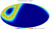 |
Fig. 1 Coverage map in time units for the LSPE-SWIPE instrumental setup assumed in this work (18 detectors for five operation days, sampled at 100 Hz). Map is in Galactic coordinates and at resolution of HEALPix Nside = 128. |
For the estimation of the angular power spectra, we followed the MASTER pseudo-Cl estimator approach (Hivon et al. 2002), that is a fast and accurate method that corrects for E/B-mode and multipoles mixings due to the partial sky coverage. Nonetheless, as mentioned by Molinari et al. (2014), at large angular scales the use of a quadratic maximum likelihood (QML) approach may be more convenient, even if much more demanding from a computational point of view. For the purposes of this work, we evaluated that the accuracy provided by the pseudo-Cl algorithm is indeed sufficient.
For any of the setups assumed here, we used an indipendent sky mask calculated from the corresponding pixel inverse condition number map, taking the values ≳10-2 (see Sect. 3.2). At this level, we did not use any mask apodisation. In addition, the power spectra were estimated according to a binning Δℓ = 10 (beside the first bin which is calculated from ℓ = 2), in such a way that the bin ranges are 2 < ℓ < 9, 10 < ℓ < 19, and so on.
3. Results
In this section we present and discuss our simulations aimed at optimizing the polarization modulation strategy of the SWIPE experiment. We tested a variety of HWP configurations, either in stepped or spinning mode, exploring two different azimuth telescope scan-speeds. In detail, we investigated the following 12 schemes:
-
an HWP stepped every 1 s, 60 s and 3600 s with the telescope scanning at 12 deg/s and 0.7 deg/s;
-
an HWP spinning with mechanical frequency of 5 Hz, 2 Hz and 0.5 Hz with, again, the telescope scanning at 12 deg/s and 0.7 deg/s.
The HWP setups listed above span the full range of the possible configurations that are currently considered experimentally feasible. The maximum telescope rotation rate is given by the gondola pendulation, the detector noise and response time, while the maximum stepped or spinning HWP rotation rates are set by mechanical feasibility and preliminary tests on the heat generation, respectively.
3.1. Periodograms
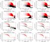 |
Fig. 2 Periodograms, i.e., plots of temperature (red) and polarization (black) intensity power as function of frequency, for the HWP setups under consideration: stepping every 1 s, 60 s and 3600 s and spinning at 5 Hz, 2 Hz and 0.5 Hz, for a telescope scanning at 12 deg/s and 0.7 deg/s. We note that the telescope rotation affects both temperature and polarization, while the HWP modulates only polarization. For a spinning HWP design, the polarization signal is shifted to higher frequencies into a narrow band centered around a frequency f = 4fr, where fr is the rotation frequency. |
A natural consequence of employing a rotating HWP is the signal modulation. In Fig. 2 we show the plots of temperature and polarization intensity power as function of frequency (periodograms) for the HWP rotation schemes under examination.
We highlight that a HWP modulates only the polarization signal, while the telescope scan-speed affects both intensity and polarization. Intensity modulation can therefore be achieved only via telescope scanning and the (small) amount of sky rotation (Brown et al. 2009).
It is clearly desirable to move the polarization power away from the low frequency 1/f noise as far as possible. Furthermore, it would be preferable to filter out the smallest amount of intensity signal, since temperature anisotropy provides a viable source of calibration by direct comparison with Planck anisotropy maps.
To better understand the meaning of the periodograms, we point out that the first peak in the temperature plots is the fundamental mode corresponding to the gondola scanning frequency, followed by its harmonics. We note that the pattern of the polarization plots in the case of a slow stepped HWP is very similar to the corresponding temperature plots, as the HWP modulation contribution is subdominant with respect to the gondola spinning. We also point out that the high-frequency tail of the periodograms has no physical meaning since is due to pixelization effects.
This analysis confirms the following general expectations: i) the ability of shifting the polarization signal to higher frequencies is typical of the spinning HWP mode. In this case the polarization power is moved to a narrow band centered at frequency f = 4fr, where fr is the rotation frequency. The bandwidth depends on both the HWP and the telescope rotation rates: in particular, we find that a narrower bandwidth corresponds to slower telescope scanning rates; ii) for a stepped HWP, the gain in the polarization signal modulation is less clear. The modulation performance is only slightly sensitive to the HWP rotation rate, while we find a moderate dependence on the telescope scan-speed.
In addition, the periodograms display an interesting feature: the “doubling” of the polarization peaks, due to the interaction of the HWP and telescope scanning strategies, which is particularly evident for some configurations (see, e.g., the stepped mode at 60 s or the spinning mode at 0.5 Hz at telescope scan-speed of 12 deg/s).
3.2. Pixel inverse condition number
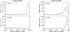 |
Fig. 3 Pixel inverse condition numbers for the HWP setups under consideration. First column: HWP stepped every 1 s (solid black line), 60 s (dotted red line) and 3600 s (dashed blue line), for a telescope scanning at 12 deg/s (top) and 0.7 deg/s (bottom). Second column: HWP spinning at 5 Hz (solid black line), 2 Hz (dotted red line) and 0.5 Hz dashed blue line), for a telescope scanning at 12 deg/s (top) and 0.7 deg/s (bottom). In our convention, the condition number Rcond has a value running from 0 to 0.5, where Rcond = 0.5 means perfect angle coverage. |
The pixel inverse condition number (hereafter, Rcond) is a useful tool to quantify the angle coverage uniformity of the observation on a given pixel. In our definition, Rcond is the ratio of the absolute values of the smallest and largest eigenvalues for each block of the preconditioner matrix employed in the map-making algorithm. In this formalism, Rcond has a value running from zero to 1/2, with Rcond = 1/2 in case of perfect angle coverage (see, e.g., Kurki-Suonio et al. 2009, for more details). We note that the condition number has a pure geometrical meaning, being essentially independent from the map-making algorithm employed. It is usually assumed that a value Rcond ≤ 10-2 means that the polarization cannot be solved and hence those pixels must be removed from the analysis. The use of a HWP modulator clearly improves the pixel angle coverage during the observation, since each pixel is observed from more directions.
In Fig. 3 we show the histograms of the pixel inverse condition number for the HWP configurations under examination. We find that: i) for a fast telescope rotation (12 deg/s), all the HWP configurations provide very good pixel angle coverage, but the slowest stepped mode (3600 s). The performance of a stepped HWP increases as its rotation rate does, while the opposite happens to a spinning HWP; ii) for a slow telescope rotation (0.7 deg/s), the performance of a stepped HWP dramatically decreases, while a spinning HWP still provides a very good pixel angle coverage. As opposite to the fast telescope rotation case, now a rapidly spinning HWP provides a better coverage than a slowly spinning one.
We conclude that a spinning scheme offers a very good pixel angle coverage for any HWP rotation frequency and any gondola scanning rate. A slow stepped HWP (3600 s) is never effective to provide a good coverage, while a fast stepping HWP (1 s and 60 s) provides a good coverage only when combined to a fast telescope scan-speed.
3.3. Map-making residuals
In this section we investigate the impact of the HWP modulation on the map reconstruction. The GLS maps are the primary output of our map-making code, but we will rather work in terms of residual maps, meaning the difference between the output optimal and the input maps. Hence, smaller residuals imply smaller map-making errors. As output maps, we considered both the signal-only (S) and signal plus noise (S+N) cases. We note that poorly observed pixels were removed from the analysis by setting a filter on the pixel inverse condition number (Rcond> 10-2).
We evaluated the residual map distribution over the angular scales by producing the corresponding BB angular power spectra (see Fig. 4). In both the S and S+N cases, the slowest HWP stepped mode (3600 s) provides higher residuals at any telescope scan-speed. Moreover, we find that the performance of a HWP stepped every 60 s worsens when a slow telescope scan-speed (0.7 deg/s) is performed. On the contrary, the residuals corresponding to the spinning HWP configurations do not significantly change against variations of both the HWP and gondola rotation rates. The residuals corresponding to the default SWIPE configuration are comparable to those of a generic spinning scheme.
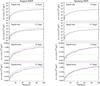 |
Fig. 4 BB angular power spectra from S (first two rows) and S+N (last two rows) residual maps for the HWP setups under consideration. First column: HWP stepped every 1 s (solid black line), 60 s (dotted red line) and 3600 s (dashed blue line), for a telescope scanning at 12 deg/s and 0.7 deg/s. Second column: HWP spinning at 5 Hz (solid black line), 2 Hz (dotted red line) and 0.5 Hz (dashed blue line), for a telescope scanning at 12 deg/s and 0.7 deg/s. The BB spectrum from the input map is shown for comparison in green dot-dashed line (in the S case the spectrum is rescaled down by a factor 104). The assumed noise level corresponds to five days and 18 detectors. |
3.4. Angular power spectra
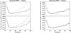 |
Fig. 5 Comparison of BB angular power spectrum error bars (in μK2) for the HWP setups under consideration. The spectra have been estimated by an implementation of the MASTER pseudo-Cl method from 50 N, S and S+N Monte Carlo maps. The error bars correspond to the standard deviation of the realizations (i.e. the dispersion of the simulations). The spectra have been produced assuming a couple of detectors for one day of operation. We note that the noise-only maps have been rescaled by a factor ~28.7, as (optimistically) expected by extending the observation to 110 detectors and 15 days. First column: HWP stepped every 1 s (solid black line), 60 s (dotted red line) and 3600 s (dashed blue line), for a telescope scanning at 12 deg/s (top) and 0.7 deg/s (bottom). Second column: HWP spinning at 5 Hz (in solid black line), 2 Hz (dotted red line) and 0.5 Hz (dashed blue line), for a telescope scanning at 12 deg/s (top) and 0.7 deg/s (bottom). |
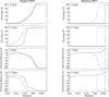 |
Fig. 6 First two rows: percentage of polarization intensity power lost when different high-pass filters are applied to the TOD as function of the cut-on frequency fc. Second two rows: fractional difference of the polarization S/N between the cases with and without high-pass filters as function of fc. The fractional difference is calculated as (S/Nfil−S/Ntot) × 100 /S/Ntot, where S/Nfil and S/Ntot refer to the cases with and without filters. We note that the polarization signal intensity is extracted directly from the plots of Fig. 2. The cut-on frequency fc is set to vary from 0.001 Hz to 50 Hz. First column: HWP stepping every 1 s (solid black line), 60 s (dotted red line) and 3600 s (dashed blue line), for a telescope scanning at 12 deg/s and 0.7 deg/s. Second column: HWP spinning at 5 Hz (solid black line), 2 Hz (dotted red line) and 0.5 Hz (dashed blue line), for a telescope scanning at 12 deg/s and 0.7 deg/s. |
We then extended to the power spectrum domain the results derived at the map-making stage.
We generated 50 noise-only (N), S and S+N Monte Carlo maps for each HWP scheme under consideration and estimate the angular power spectra following the MASTER pseudo-Cl estimator method. To reduce the computational requirements, the maps were produced assuming two detectors for one day of operation (at telescope elevation of 35 deg).
We note that the noise-only maps have been rescaled by a factor ~28.7, as (optimistically) expected by extending the observation to 110 detectors and 15 days. In Fig. 5 we compare the full (i.e., cosmic variance plus noise) BB spectrum error bars for the HWP configuration under analysis.
We find that, in agreement with the residual analysis, a slow stepped HWP provides larger spectrum standard deviations at any telescope rotation rate, and that the performance of a stepped configuration worsens by slowing down the gondola scan-speed. We stress that the low number of Monte Carlo maps considered here impacts on the accuracy of the spectrum error bars at the very large angular scales. The optimal estimate of the low-multipole power spectra is beyond the scope of this paper and will be addressed in a forthcoming work.
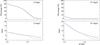 |
Fig. 7 Percentage of polarization intensity power lost when different band-pass filters are applied (first row) and ratios of the polarization S/N between the cases with and without band-pass filters (second row). The bandwidth of the filter Δf = (fmax−fmin)/2 is set to vary from 0.1 Hz to 5 Hz around the peak frequency (four times the rotation frequency). Plots are for a HWP spinning at 5 Hz (solid black line), 2 Hz (dotted red line) and 0.5 Hz (dashed blue line), for a telescope scanning at 12 deg/s and 0.7 deg/s. |
3.5. High-pass filters
It is important to test the HWP configurations against a possible filtering of the low-frequency data streams, which is a common practice to cut the 1/f part of the noise spectrum in order to maximize the signal-to-noise ratio (S/N). It is beyond the aim of this work to forecast a filtering strategy for the SWIPE experiment, nonetheless it is interesting to investigate how the polarization modulation could impact on the choice of a suitable data stream filter.
In choosing a proper filter, two parameters must be accounted for: the fraction of signal lost and the increase in the S/N. In Fig. 6 we show the percentage of polarization intensity power that would be cut out from different high-pass filters, for the HWP schemes under consideration. The cut-on frequency fc was set to vary from 10-3 Hz to 50 Hz. It is also shown the fractional difference of the (polarization) S/N between the cases with and without high-pass filters.
Due to the shift of the polarization signal to higher frequencies, a spinning HWP clearly allows much more freedom in the choice of the cut-on frequency: fc can be freely chosen sufficiently below the peak frequency with no loss in cosmological signal. For instance, we find that, in order to preserve at least 90% of the polarization signal, the maximum allowed cut-on frequency for the nominal configuration is around fc = 0.03 Hz, while for a fast spinning scheme (5 Hz) almost fc = 20 Hz. This implies that, for the nominal modulation setup, the increase in S/N with respect to the no filter case cannot be more than a factor 20%, while with a fast spinning HWP we can gain a factor 40–50%.
We finally quantified the impact of a typical high-pass filter (fc = 0.1 Hz; see, e.g., Masi et al. 2006) on the polarization map recovery. We generated maps from the filtered TOD and calculate the residuals (for both the S and S+N cases) and the corresponding BB angular power spectra. As expected, the spinning mode is not generally affected by the presence of this specific filter. On the contrary, the impact on the stepped HWP setups is very large: we find a raise in the BB residual spectrum up to six and three orders of magnitude for the S and S+N cases, respectively. This increase is generally more prominent at large scales.
3.6. Band-pass filters
A spinning HWP scheme allows for the interesting possibility of using a band-pass filter. The frequency band is centered around the peak frequency (see Fig. 2), that is at 4fr, where fr is the spinning frequency. We explored the effect of a set of band-pass filter by calculating the percentage of polarization intensity power lost and the associated S/N as function of the filter bandwidth Δf = (fmax−fmin)/2, where Δf is set to vary from 0.1 Hz to 5 Hz. Results are shown in Fig. 7. In particular we plot the ratio of the S/N between the cases with and without filters.
While we do not find any relevant dependence on the HWP rotation frequency, the telescope scan-speed has a large effect. We notice a higher S/N when slower telescope scan-speeds are performed: this is because, as shown in Fig. 2, the bandwidths are narrower in this case.
For instance, if we want to preserve the 90% of the cosmological signal, we need a bandwidth of at least ~2 Hz and 0.1 Hz for a telescope scanning at 12 deg/s and 0.7 deg/s, respectively. The S/N will consequently increase: it will reach a value of ~4 and ~18 times the reference S/N calculated without any filter, respectively.
3.7. Minimal observation case
We then compared the HWP performance in the minimal observation case (one detector for one operation day), which is a crucial test for single-detector calibration purposes. The basic strategy for LSPE-SWIPE in-flight calibration is described in (de Bernardis et al. 2012). Around one day of the mission will be devoted to calibration scans. We generated then maps assuming one detector and one day of operation and calculate the residuals. We find that the differences among the various HWP designs are much larger than in the previous two focal plane simulations.
Results confirm that some stepped HWP configurations are strongly disfavored. For instance, a slowly stepped configuration provides S BB residual spectra with an amplitude orders of magnitude larger than other setups. Furthermore, we now find non-negligible differences between fast stepped modes (when combined with a rapid telescope scan-speed) and spinning modes.
As an example, in Fig. 8 we show S and S+N BB residual spectra for the nominal HWP strategy, for two continuously rotating configurations (slowly spinning at 0.5 Hz with a fast gondola rotation of 12 deg/s, and rapidly spinning at 5 Hz with a slow telescope scanning rate of 0.7 deg/s) and for a slowly stepped HWP (3600 s, combined with a slow gondola scanning frequency of 0.7 deg/s).
In the S case, we find that the two spinning modes are slighly more effective in recovering polarization with respect to the nominal configuration at any scale. In particular, the difference increases after ℓ ≳ 100. In the S+N case, we find a large discrepancy between the nominal and the spinning schemes at very low multipoles, while the difference is damped at smaller scales.
3.8. HWP-induced systematics
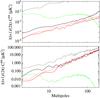 |
Fig. 8 BB angular power spectra from S (on the top) and S+N (on the bottom) residual maps for the minimal case of one detector and one operation day. HWP stepped every 60 s with a telescope scanning rate of 12 deg/s (solid black line); HWP stepped every 3600 s with a telescope scanning rate of 0.7 deg/s (dashed black line); HWP spinning at 5 Hz with a telescope scanning rate of 0.7 deg/s (solid red line); HWP spinning at 0.5 Hz with a telescope scanning rate of 12 deg/s (dashed red line). The BB spectrum from the input map is shown for comparison by the green dot-dashed line (in the S case the spectrum is rescaled down by a factor of 102). |
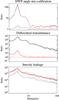 |
Fig. 9 Ratio of S residual BB angular power spectra between the cases with and without HWP-induced systematic effects. Top panel: HWP angle miscalibration of amplitude 0.1° RMS (solid line) and 0.01° RMS (dashed line). Middle panel: differential transmittance between the two orthogonal states of amplitude 1%, producing both a Q and U mis-calibration and an intensity leakage modulated at 2fr (solid line), only the former (dotted line), only the latter (dashed line). Bottom panel: generic intensity leakage of amplitude 5% modulated both at 2 and 4fr (solid line), only at 2fr (dotted line), only at 4fr (dashed line). Two HWP configurations are considered: the nominal LSPE-SWIPE stepped setup (black) and a fast spinning design (rotating at 5 Hz with a slow gondola scanning at 0.7 deg/s, in red). |
In the simulations above we assumed an ideal HWP, meaning that it did not introduce systematic effects of its own. In this section we investigate the impact of typical HWP-induced systematics on the B-mode polarization recovery. In particular, we explored the effects of: i) a mis-estimation of the HWP angles; ii) a possible differential transmittance between the two orthogonal states; iii) a leakage from temperature to polarization, arising, for instance, from an imperfect optical setup.
We limited ourselves to the default LSPE-SWIPE stepped configuration and a fast spinning design (rotating at 5 Hz, with a slow gondola scanning rate of 0.7 deg/s). As example of HWP angle mis-estimation, we simulated the effect of both a random error and a systematic offset on the HWP angles. As pessimistic (optimistic) case, we considered both these systematics to have an amplitude of 0.1° (0.01°) RMS. As figure of merit, we used the recovered BB power spectra from S residual maps. In Fig. 9 we show the ratio of the BB residuals between the cases with and without the HWP angle mis-calibration, for the two chosen error amplitudes and for the two HWP configurations under exam.
First, we notice that the impact of the HWP angle error is independent on the HWP configuration: this is in agreement with the results presented in Brown et al. (2009). When considering separately the random error and the systematic offset, we find that the impact of the former is negligible with respect the latter. Moreover, as we show, a HWP angle error can potentially cause a large increase in the BB residuals at the largest scales (ℓ ≲ 10). An accuracy of better 0.01° RMS is therefore needed for the systematic offset to avoid any bias in the large scale B-mode recovery. In LSPE-SWIPE, around 80 detectors will be devoted to constantly monitor the HWP position, making this requirement achievable.
As second example of HWP systematic effect, we considered a differential transmittance between the two orthogonal states of amplitude δ = 1%. At first order, this implies a miscalibration of Q and U and a leakage from I modulated at 2fr (see Brown et al. 2009). In Fig. 9 we show the ratio of BB residual spectra between the cases with and without differential transmittance. Confirming the general expectation, we find that the effect of the polarization mis-calibration is sub-dominant and independent on the HWP setup. The intensity leakage is particularly worrisome in the stepped HWP case since it causes an increase of the BB residuals of up to four or five orders of magnitude (at large scales), while its impact is drastically reduced in a spinning scheme, as the signal is instead modulated at 4fr.
Finally, we considered a possible leakage from I to Q and U of amplitude α = 5%, that can be sourced, for instance, by internal reflections of linearly polarized light between the polarizer and the HWP (Salatino & de Bernardis 2010). In this case, the spurious polarization is modulated both at 2 and 4fr. In Fig. 9 we display the ratio of BB residual spectra between the cases with and without leakage, where we also compare the separate effects of the two modulated leakage modes. As expected, we find that only the contribution at 4fr impacts on the spinning HWP performance, while both the 2 and 4fr contributions affect a stepped HWP. Nonetheless, the overall effect is comparable in the two configurations.
When decreasing the intensity leakage to an amplitude α = 1%, we find that the BB residual level is rescaled by only an order of magnitude. Sophisticated techniques aimed at minimizing the intensity-polarization coupling (see, e.g., Wallis et al. 2015) will therefore represent a crucial issue.
4. Conclusions
In this work we present preliminary forecasts of the LSPE-SWIPE experiment with the final goal to optimize the HWP polarization modulation strategy. We departed from the nominal SWIPE modulation strategy (stepped every 60 s with telescope scan-speed 12 deg/s) and perform a detailed investigation of a wide range of possible HWP rotation schemes, either in stepped (every 1 s, 60 s and 3600 s) or spinning (at rate 5 Hz, 2 Hz, 0.5 Hz) mode, allowing for two different azimuth telescope scan-speeds (12 deg/s and 0.7 deg/s).
We explored the response of the different HWP setups in the frequency, map and angular power spectrum domains. Maps are generated by the optimal ROMA MPI-parallel algorithm. Spectra are estimated using an implementation of the MASTER pseudo-Cl method. Our analysis accounts for a 1/f low-frequency noise both self-correlated and cross-correlated among the polarimeters.
Furthermore, we quantify the effect of high-pass and band-pass filters of the data stream. In particular, we show that a band-pass filter is a very interesting possibility, as it enables to achieve a remarkably higher S/N with respect to the more common high-pass filters, especially when a slow telescope modulation is performed. We finally analyzed the minimal observation case (one detector for one day of operation), critical for the single-detector calibration process, and test the HWP performance against typical HWP-induced systematics.
In terms of pixel angle coverage, map-making residuals (S and S+N) and BB power spectrum standard deviations, we find that a slowly stepped HWP (≳3600 s) provides much poorer performance and that the performance of a stepped HWP drastically worsens when slowing down the telescope scan-speed. Therefore, even if they are easiest to operate, these configurations must be rejected from further investigation. At fast telescope scan-speed, we find no difference between a HWP stepped every 1 s or 60 s, making the nominal configuration the best option among the set of stepped schemes.
The performance of a spinning HWP is not very sensitive on both the HWP rotation rate and the gondola scanning frequency. Moreover, the various spinning designs provide comparable results to the default stepped modulation strategy.
However, we find that the nominal SWIPE configuration may not be the most convenient choice when accounting for some specific real-case situations. For instance, a rapidly spinning HWP scheme (5 Hz) combined with a slow telescope modulation rate (0.7 deg/s) provides the highest performance in presence of high-pass and band-pass filters since the polarization signal is shifted to very high frequencies into a very narrow band.
In order to preserve 90% of polarization signal information, any high-pass filter could at most increase the S/N of less than 20% and up to 40–50%, for the nominal modulation case and for a HWP spinning at 5 Hz, respectively. Moreover, for any spinning setup combined with a gondola scanning at 0.7 deg/s, a band-pass filter could increase the S/N up to approximately 18 times, without losing more than 10% of polarization power.
In addition, this specific spinning design allows a more efficient polarization recovery in the case of one detector-one operation day. The corresponding S BB residuals are lower at any angular scales with respect to the nominal HWP configuration. In the S+N case we find an improvement at the lowest multipoles while the difference is damped at smaller scales.
When including systematics intrinsic to the HWP, we find that any spurious polarization contribution (arising for instance from differential transmittance or imperfect optical setup) modulated at twice the HWP rotation frequency is completely suppressed by a spinning mode, while it can largely affect the performance of a stepped configuration (at large scales). This is expected, as in the spinning case the polarization signal is modulated at four times the spinning rate. Instead, when considering realistic HWP angle errors, Q and U mis-calibration due to differential transmittance, and generic leakage from I to Q and U modulated at four times the rotation frequency, we find no relevant difference between the stepped and spinning mode responses.
The range of HWP-induced systematics analyzed here is not exhaustive. In addition, in this work we did not account for other instrumental systematic effects (e.g., pointing errors and calibration drifts). To draw final conclusions, a detailed investigation of these issues is required and left to future work.
Although the simulations presented in this paper are specific to the SWIPE instrument, our results are qualitatively valid for any scanning telescope B-mode mission aiming at large angular scales.
Acknowledgments
The LSPE project is supported by the contract I/022/11/0 of the Italian Space Agency and by INFN CSN2. We acknowledge the use of the HEALPix package (Górski et al. 2005), the CAMB software (Lewis & Bridle 2002) and the FFTW library (Frigo & Johnson 2005). We acknowledge the CINECA award under the ISCRA initiative, for the availability of high performance computing resources and support. This research used resources of the National Energy Research Scientific Computing Center (NERSC), which is supported by the Office of Science of the U.S. Department of Energy under Contract No. DE-AC02-05CH11231. AB thanks Fabio Columbro for useful discussions. We finally wish to thank the LSPE collaboration and the anonymous referee for useful suggestions.
References
- Ade, P. A. R., Akiba, Y., Anthony, A. E., et al. 2014, Phys. Rev. Lett., 113, 021301 [NASA ADS] [CrossRef] [Google Scholar]
- Aiola, S., Amico, G., Battaglia, P., et al. 2012, SPIE Conf. Ser., 8446, 7 [Google Scholar]
- Arnold, K., Ade, P. A. R., Anthony, A. E., et al. 2010, in Millimeter, Submillimeter, and Far-Infrared Detectors and Instrumentation for Astronomy V, Proc. SPIE, 7741, 77411E [CrossRef] [Google Scholar]
- Bersanelli, M., Mennella, A., Morgante, G., et al. 2012, in SPIE Conf. Ser., 8446, 7 [Google Scholar]
- BICEP2/Keck and Planck Collaborations 2015, Phys. Rev. Lett., 114, 101301 [NASA ADS] [CrossRef] [PubMed] [Google Scholar]
- Brown, M. L., Challinor, A., North, C. E., et al. 2009, MNRAS, 397, 634 [NASA ADS] [CrossRef] [Google Scholar]
- Bryan, S. A., Ade, P. A. R., Amiri, M., et al. 2010, in Millimeter, Submillimeter, and Far-Infrared Detectors and Instrumentation for Astronomy V, Proc. SPIE, 7741, 77412B [CrossRef] [Google Scholar]
- Buzzelli, A., Cabella, P., de Gasperis, G., & Vittorio, N. 2016, J. Phys. Conf. Ser., 689, 012003 [NASA ADS] [CrossRef] [Google Scholar]
- Buzzelli, A., de Gasperis, G., de Bernardis, P., Masi, S., & Vittorio, N. 2017, J. Phys. Conf. Ser., 841, 012001 [CrossRef] [Google Scholar]
- de Bernardis, P., Aiola, S., Amico, G., et al. 2012,SPIE Conf. Ser., 8452, 3 [Google Scholar]
- de Gasperis, G., Balbi, A., Cabella, P., Natoli, P., & Vittorio, N. 2005, A&A, 436, 1159 [NASA ADS] [CrossRef] [EDP Sciences] [Google Scholar]
- de Gasperis, G., Buzzelli, A., Cabella, P., de Bernardis, P., & Vittorio, N. 2016, A&A, 593, A15 [NASA ADS] [CrossRef] [EDP Sciences] [Google Scholar]
- Filippini, J. P., Ade, P. A. R., Amiri, M., et al. 2010, in Millimeter, Submillimeter, and Far-Infrared Detectors and Instrumentation for Astronomy V, Proc. SPIE, 7741, 77411N [CrossRef] [Google Scholar]
- Frigo, M., & Johnson, S. G. 2005, special issue on Program Generation, Optimization, and Platform Adaptation, Proc IEEE, 93, 216, [Google Scholar]
- Górski, K. M., Hivon, E., Banday, A. J., et al. 2005, ApJ, 622, 759 [NASA ADS] [CrossRef] [Google Scholar]
- Gualtieri, R., Battistelli, E. S., Cruciani, A., et al. 2016, J. Low Temp. Phys., 184, 527 [Google Scholar]
- Hill, C. A., Beckman, S., Chinone, Y., et al. 2016, Proc. SPIE, 9914, 99142U [CrossRef] [Google Scholar]
- Hinshaw, G., Larson, D., Komatsu, E., et al. 2013, ApJS, 208, 19 [NASA ADS] [CrossRef] [Google Scholar]
- Hivon, E., Górski, K. M., Netterfield, C. B., et al. 2002, ApJ, 567, 2 [NASA ADS] [CrossRef] [Google Scholar]
- Hu, W., Hedman, M. M., & Zaldarriaga, M. 2003, Phys. Rev. D, 67, 043004 [NASA ADS] [CrossRef] [Google Scholar]
- Johnson, B. R., Collins, J., Abroe, M. E., et al. 2007, ApJ, 665, 42 [NASA ADS] [CrossRef] [Google Scholar]
- Kamionkowski, M., Kosowsky, A., & Stebbins, A. 1997, Phys. Rev. Lett., 78, 2058 [NASA ADS] [CrossRef] [Google Scholar]
- Keck Array, BICEP2 Collaborations, et al. 2016, ApJ, 833, 228 [NASA ADS] [CrossRef] [Google Scholar]
- Kovac, J. M., Leitch, E. M., Pryke, C., et al. 2002, Nature, 420, 772 [NASA ADS] [CrossRef] [PubMed] [Google Scholar]
- Kurki-Suonio, H., Keihänen, E., Keskitalo, R., et al. 2009, A&A, 506, 1511 [NASA ADS] [CrossRef] [EDP Sciences] [Google Scholar]
- Lewis, A., & Bridle, S. 2002, Phys. Rev. D, 66, 103511 [NASA ADS] [CrossRef] [Google Scholar]
- Lyth, D. H. D. H., & Riotto, A. A. 1999, Phys. Rep., 314, 1 [Google Scholar]
- MacTavish, C. J., Ade, P. A. R., Bock, J. J., et al. 2006, ApJ, 647, 799 [NASA ADS] [CrossRef] [Google Scholar]
- MacTavish, C. J., Ade, P. A. R., Battistelli, E. S., et al. 2008, ApJ, 689, 655 [NASA ADS] [CrossRef] [Google Scholar]
- Masi, S., Ade, P. A. R., Bock, J. J., et al. 2006, A&A, 458, 687 [NASA ADS] [CrossRef] [EDP Sciences] [Google Scholar]
- Matsumura, T., Akiba, Y., Borrill, J., et al. 2014, J. Low Temp. Phys., 176, 733 [NASA ADS] [CrossRef] [Google Scholar]
- Molinari, D., Gruppuso, A., Polenta, G., et al. 2014, MNRAS, 440, 957 [NASA ADS] [CrossRef] [Google Scholar]
- Montroy, T. E., Ade, P. A. R., Bock, J. J., et al. 2006, ApJ, 647, 813 [NASA ADS] [CrossRef] [Google Scholar]
- O’Dea, D., Challinor, A., & Johnson, B. R. 2007, MNRAS, 376, 1767 [NASA ADS] [CrossRef] [Google Scholar]
- Oxley, P., Ade, P. A., Baccigalupi, C., et al. 2004, in Infrared Spaceborne Remote Sensing XII, ed. M. Strojnik, Proc. SPIE, 5543, 320 [Google Scholar]
- Patanchon, G., Ade, P. A. R., Bock, J. J., et al. 2008, ApJ, 681, 708 [NASA ADS] [CrossRef] [Google Scholar]
- Planck Collaboration XI. 2016, A&A 594, A11 [NASA ADS] [CrossRef] [EDP Sciences] [Google Scholar]
- Planck Collaboration XIII. 2016, A&A, 594, A13 [NASA ADS] [CrossRef] [EDP Sciences] [Google Scholar]
- Planck Collaboration Int. XLI. 2016, A&A, 596, A102 [NASA ADS] [CrossRef] [EDP Sciences] [Google Scholar]
- Planck Collaboration Int. XLVI. 2016, A&A, 596, A107 [NASA ADS] [CrossRef] [EDP Sciences] [Google Scholar]
- Qubic Collaboration, Battistelli, E., Baú, A., et al. 2011, Astropart. Phys., 34, 705 [NASA ADS] [CrossRef] [Google Scholar]
- Salatino, M., & de Bernardis, P. 2010, ArXiv e-prints [arXiv:1006.3225] [Google Scholar]
- Simon, S. M., Appel, J. W., Campusano, L. E., et al. 2016, J. Low Temp. Phys., 184, 534 [NASA ADS] [CrossRef] [Google Scholar]
- Spergel, D. N., Verde, L., Peiris, H. V., et al. 2003, ApJS, 148, 175 [NASA ADS] [CrossRef] [Google Scholar]
- The COrE Collaboration, Armitage-Caplan, C., Avillez, M., et al. 2011, ArXiv e-prints [arXiv:1102.2181] [Google Scholar]
- Wallis, C. G. R., Bonaldi, A., Brown, M. L., & Battye, R. A. 2015, MNRAS, 453, 2058 [NASA ADS] [CrossRef] [Google Scholar]
- Wu, W. L. K., Ade, P. A. R., Ahmed, Z., et al. 2016, J. Low Temp. Phys., 184, 765 [NASA ADS] [CrossRef] [Google Scholar]
- Zaldarriaga, M., & Seljak, U. 1998, Phys. Rev. D, 58, 023003 [NASA ADS] [CrossRef] [Google Scholar]
All Figures
|
Fig. 1 Coverage map in time units for the LSPE-SWIPE instrumental setup assumed in this work (18 detectors for five operation days, sampled at 100 Hz). Map is in Galactic coordinates and at resolution of HEALPix Nside = 128. |
| In the text | |
|
Fig. 2 Periodograms, i.e., plots of temperature (red) and polarization (black) intensity power as function of frequency, for the HWP setups under consideration: stepping every 1 s, 60 s and 3600 s and spinning at 5 Hz, 2 Hz and 0.5 Hz, for a telescope scanning at 12 deg/s and 0.7 deg/s. We note that the telescope rotation affects both temperature and polarization, while the HWP modulates only polarization. For a spinning HWP design, the polarization signal is shifted to higher frequencies into a narrow band centered around a frequency f = 4fr, where fr is the rotation frequency. |
| In the text | |
|
Fig. 3 Pixel inverse condition numbers for the HWP setups under consideration. First column: HWP stepped every 1 s (solid black line), 60 s (dotted red line) and 3600 s (dashed blue line), for a telescope scanning at 12 deg/s (top) and 0.7 deg/s (bottom). Second column: HWP spinning at 5 Hz (solid black line), 2 Hz (dotted red line) and 0.5 Hz dashed blue line), for a telescope scanning at 12 deg/s (top) and 0.7 deg/s (bottom). In our convention, the condition number Rcond has a value running from 0 to 0.5, where Rcond = 0.5 means perfect angle coverage. |
| In the text | |
|
Fig. 4 BB angular power spectra from S (first two rows) and S+N (last two rows) residual maps for the HWP setups under consideration. First column: HWP stepped every 1 s (solid black line), 60 s (dotted red line) and 3600 s (dashed blue line), for a telescope scanning at 12 deg/s and 0.7 deg/s. Second column: HWP spinning at 5 Hz (solid black line), 2 Hz (dotted red line) and 0.5 Hz (dashed blue line), for a telescope scanning at 12 deg/s and 0.7 deg/s. The BB spectrum from the input map is shown for comparison in green dot-dashed line (in the S case the spectrum is rescaled down by a factor 104). The assumed noise level corresponds to five days and 18 detectors. |
| In the text | |
|
Fig. 5 Comparison of BB angular power spectrum error bars (in μK2) for the HWP setups under consideration. The spectra have been estimated by an implementation of the MASTER pseudo-Cl method from 50 N, S and S+N Monte Carlo maps. The error bars correspond to the standard deviation of the realizations (i.e. the dispersion of the simulations). The spectra have been produced assuming a couple of detectors for one day of operation. We note that the noise-only maps have been rescaled by a factor ~28.7, as (optimistically) expected by extending the observation to 110 detectors and 15 days. First column: HWP stepped every 1 s (solid black line), 60 s (dotted red line) and 3600 s (dashed blue line), for a telescope scanning at 12 deg/s (top) and 0.7 deg/s (bottom). Second column: HWP spinning at 5 Hz (in solid black line), 2 Hz (dotted red line) and 0.5 Hz (dashed blue line), for a telescope scanning at 12 deg/s (top) and 0.7 deg/s (bottom). |
| In the text | |
|
Fig. 6 First two rows: percentage of polarization intensity power lost when different high-pass filters are applied to the TOD as function of the cut-on frequency fc. Second two rows: fractional difference of the polarization S/N between the cases with and without high-pass filters as function of fc. The fractional difference is calculated as (S/Nfil−S/Ntot) × 100 /S/Ntot, where S/Nfil and S/Ntot refer to the cases with and without filters. We note that the polarization signal intensity is extracted directly from the plots of Fig. 2. The cut-on frequency fc is set to vary from 0.001 Hz to 50 Hz. First column: HWP stepping every 1 s (solid black line), 60 s (dotted red line) and 3600 s (dashed blue line), for a telescope scanning at 12 deg/s and 0.7 deg/s. Second column: HWP spinning at 5 Hz (solid black line), 2 Hz (dotted red line) and 0.5 Hz (dashed blue line), for a telescope scanning at 12 deg/s and 0.7 deg/s. |
| In the text | |
|
Fig. 7 Percentage of polarization intensity power lost when different band-pass filters are applied (first row) and ratios of the polarization S/N between the cases with and without band-pass filters (second row). The bandwidth of the filter Δf = (fmax−fmin)/2 is set to vary from 0.1 Hz to 5 Hz around the peak frequency (four times the rotation frequency). Plots are for a HWP spinning at 5 Hz (solid black line), 2 Hz (dotted red line) and 0.5 Hz (dashed blue line), for a telescope scanning at 12 deg/s and 0.7 deg/s. |
| In the text | |
|
Fig. 8 BB angular power spectra from S (on the top) and S+N (on the bottom) residual maps for the minimal case of one detector and one operation day. HWP stepped every 60 s with a telescope scanning rate of 12 deg/s (solid black line); HWP stepped every 3600 s with a telescope scanning rate of 0.7 deg/s (dashed black line); HWP spinning at 5 Hz with a telescope scanning rate of 0.7 deg/s (solid red line); HWP spinning at 0.5 Hz with a telescope scanning rate of 12 deg/s (dashed red line). The BB spectrum from the input map is shown for comparison by the green dot-dashed line (in the S case the spectrum is rescaled down by a factor of 102). |
| In the text | |
|
Fig. 9 Ratio of S residual BB angular power spectra between the cases with and without HWP-induced systematic effects. Top panel: HWP angle miscalibration of amplitude 0.1° RMS (solid line) and 0.01° RMS (dashed line). Middle panel: differential transmittance between the two orthogonal states of amplitude 1%, producing both a Q and U mis-calibration and an intensity leakage modulated at 2fr (solid line), only the former (dotted line), only the latter (dashed line). Bottom panel: generic intensity leakage of amplitude 5% modulated both at 2 and 4fr (solid line), only at 2fr (dotted line), only at 4fr (dashed line). Two HWP configurations are considered: the nominal LSPE-SWIPE stepped setup (black) and a fast spinning design (rotating at 5 Hz with a slow gondola scanning at 0.7 deg/s, in red). |
| In the text | |
Current usage metrics show cumulative count of Article Views (full-text article views including HTML views, PDF and ePub downloads, according to the available data) and Abstracts Views on Vision4Press platform.
Data correspond to usage on the plateform after 2015. The current usage metrics is available 48-96 hours after online publication and is updated daily on week days.
Initial download of the metrics may take a while.