| Issue |
A&A
Volume 608, December 2017
|
|
|---|---|---|
| Article Number | A136 | |
| Number of page(s) | 14 | |
| Section | Numerical methods and codes | |
| DOI | https://doi.org/10.1051/0004-6361/201731828 | |
| Published online | 15 December 2017 | |
LEAP: Looking beyond pixels with continuous-space EstimAtion of Point sources
1 École polytechnique fédérale de Lausanne, 1015 Lausanne, Switzerland
e-mail: This email address is being protected from spambots. You need JavaScript enabled to view it.
2 IBM Research Zürich, 8803 Rüschlikon, Switzerland
3 The Chinese University of Hong Kong, Shatin, NT, Hong Kong, PR China
Received: 25 August 2017
Accepted: 16 October 2017
Abstract
Context. Two main classes of imaging algorithms have emerged in radio interferometry: the CLEAN algorithm and its multiple variants, and compressed-sensing inspired methods. They are both discrete in nature, and estimate source locations and intensities on a regular grid. For the traditional CLEAN-based imaging pipeline, the resolution power of the tool is limited by the width of the synthesized beam, which is inversely proportional to the largest baseline. The finite rate of innovation (FRI) framework is a robust method to find the locations of point-sources in a continuum without grid imposition. The continuous formulation makes the FRI recovery performance only dependent on the number of measurements and the number of sources in the sky. FRI can theoretically find sources below the perceived tool resolution. To date, FRI had never been tested in the extreme conditions inherent to radio astronomy: weak signal / high noise, huge data sets, large numbers of sources.
Aims. The aims were (i) to adapt FRI to radio astronomy, (ii) verify it can recover sources in radio astronomy conditions with more accurate positioning than CLEAN, and possibly resolve some sources that would otherwise be missed, (iii) show that sources can be found using less data than would otherwise be required to find them, and (iv) show that FRI does not lead to an augmented rate of false positives.
Methods. We implemented a continuous domain sparse reconstruction algorithm in Python. The angular resolution performance of the new algorithm was assessed under simulation, and with visibility measurements from the LOFAR telescope. Existing catalogs were used to confirm the existence of sources.
Results. We adapted the FRI framework to radio interferometry, and showed that it is possible to determine accurate off-grid point-source locations and their corresponding intensities. In addition, FRI-based sparse reconstruction required less integration time and smaller baselines to reach a comparable reconstruction quality compared to a conventional method. The achieved angular resolution is higher than the perceived instrument resolution, and very close sources can be reliably distinguished. The proposed approach has cubic complexity in the total number (typically around a few thousand) of uniform Fourier data of the sky image estimated from the reconstruction. It is also demonstrated that the method is robust to the presence of extended-sources, and that false-positives can be addressed by choosing an adequate model order to match the noise level.
Key words: techniques: interferometric / methods: numerical / techniques: image processing
© ESO, 2017
1. Introduction
Existing radio interferometric imaging algorithms are discrete in nature, e.g., CLEAN (Högbom 1974) and its numerous variants (Bhatnagar & Cornwell 2004; Cornwell et al. 2008) or the compressed sensing inspired methods proposed by Wiaux et al. (2010), Starck et al. (2010), Carrillo et al. (2014), Dabbech et al. (2015). As such, they estimate the locations and intensities of celestial sources on a uniform grid that is artificially imposed over the field of view (Schwab 1984).
Sources do not line up so conveniently in reality, located instead in-between pixels of the pre-defined grid. This leads to inaccurate source position and intensity estimation, with contributions from closely located sources being merged together into a single pixel (see Fig. 1 for an illustration). Depending on the ultimate goal (e.g., calibration), it may be desired to have more accurate location estimates (and thus distances between objects) than achievable on a grid.
The starting point for this work was hence to see if we could accurately determine the intensities and locations of sources directly from visibility data without a grid imposition in an intermediate image domain. The framework commonly referred to as finite rate of innovation (FRI) sampling is a natural candidate for this task. Introduced first in the signal processing community, FRI sampling generalizes the Shannon sampling theorem to sparse non-bandlimited signals. Vetterli et al. (2002) proposed, for example, a sampling scheme permitting the exact recovery of a stream of Dirac from a few Fourier series coefficients. The framework has since been applied successfully in other fields, and extended to 2D signals as well as noisy measurements (Maravić & Vetterli 2005; Shukla & Dragotti 2007; Pan et al. 2014; Ongie & Jacob 2016). Having been originally designed to work only with equally spaced Fourier samples as input, Pan et al. (2017b) extended the FRI framework to cases with non-uniform samples (as is the case in radio interferometry). It thus becomes possible to envisage an FRI-based approach in radio astronomy, albeit with the substantial remaining challenge of recovering a large number of sources given the very weak signals and massive data sets.
A continuously defined framework such as FRI, allows the significance of the notion of achievable angular resolution to be revisited. Indeed, for the traditional CLEAN-based imaging pipeline, the resolution power of the tool, or the ability to distinguish neighboring sources, is limited by the width of the synthesized beam, whose width is inversely proportional to the longest baseline of the interferometer. Sources closer than this critical beam width are indistinguishable from one another.
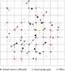 |
Fig. 1 Existing imaging algorithms estimate the locations and intensities of celestial sources on a uniform gird. In practice, sources do not line up so conveniently, and can fall off-grid. Gridding hence results in a less accurate estimation of the location estimations as well as a potential overestimation of intensities due to multiple sources being merged to the same pixel. |
In comparison, the FRI-based sparse recovery allows sources separated by a distance smaller than this apparent bound to be distinguished. The continuous-domain formulation makes the performance only dependent on the number of measurements and sources in the sky, but not on the number of pixels from an arbitrarily imposed, and potentially very large, grid. We name the proposed FRI-based approach as Looking beyond pixels with continuous-space EstimAtion of Point sources (LEAP).
Compressed sensing (e.g., Starck et al. 2010), while it surpasses the instrument resolution limit as well, does rely on a grid. LEAP differs in that the estimation of source locations is decoupled from the estimation of their intensities. Hence, it is possible to exploit the consistency in source locations among different frequency sub-bands and have a coherent reconstruction in a multi-band setting (see Sect. 2.3.3).
The present work quantifies how successfully LEAP can be applied to recover point sources in realistic radio astronomy conditions. Our experiments, carried out through simulation and actual interferometric measurements from LOFAR, show that the reconstruction is more accurate and requires fewer measurements, reaching a comparable source estimate to CLEAN from much less integration time and smaller baselines. The achievable position accuracy goes below the perceived angular resolution, which allows closely located sources to be reliably distinguished. To confirm that these super-resolved sources were indeed actual sources, we showed that CLEAN could also recover them given longer baselines (and hence sharpening its PSF). Finally, we showed that LEAP could leverage together the information from multiple frequency bands in a coherent fashion to improve point source estimation.
The paper is organized as follows. After a briefly review of the radio interferometer measurement equation in Sect. 2.1, we propose to adapt the sparse recovery framework based on FRI sampling (Sect. 2.2) to source estimations in radioastronomy in Sect. 2.3. The algorithmic details for the reconstruction of the source locations and intensities are discussed in Sects. 2.3.1 and 2.3.2. Further, we present the multi-band formulation in Sect. 2.3.3. The method is validated with both synthetic experiments (Sects. 3.2 to 3.4), actual LOFAR observations from the Boötes field (Sect. 3.5), and the “Toothbrush” cluster (Sect. 3.6), respectively. We discuss the advantages and limitations in Sect. 4 before concluding the work with a few possible future directions in Sect. 5.
2. Methods
2.1. Interferometric imaging measurement equation
A typical radio interferometer consists of an array of antennas that collect the electromagnetic waves emitted by celestial sources. In the far field context, these sources are assumed to be located on a hypothetical celestial sphere and the emitted electromagnetic waves arrive at each antenna in parallel. Consequently, the signals received at two antennas differ only by a geometric time delay, which is determined by the baseline of the antenna pair and the observation frequency. When the field-of-view is sufficiently narrow, the celestial sphere can be approximated locally by a tangential plane. It can be shown that the visibility measurements Vij, given by the cross-correlations of antenna pairs (i,j), then correspond to a 2D Fourier domain (conventionally referred to as (u,v)-domain) sampling of the sky brightness distribution I (Thompson et al. 2001; Taylor et al. 1999; Simeoni 2015): 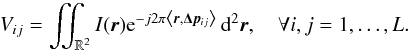 (1)Here, L is the total number of antennas forming the interferometer; r = (l,m) are the spatial coordinates of the sky image; and Δp = (pi−pj) /λ: = (uij/ 2π,vij/ 2π) is the projection onto the tangent plane of the baseline between antenna i and j, normalized by the wavelength λ of the received electromagnetic waves. For simplicity, we assumed antennas have uniform gains and omni-directional primary beams in (1). The w-term (see Cornwell et al. 2008) is considered as a constant for all baselines in a sufficiently small field-of-view. However, the proposed algorithm can straightforwardly be extended to more complex data models such as the ones considered in Simeoni (2015).
The measurement Eq. (1)is known as the van Cittert-Zernike theorem (Thompson et al. 2001, Chap. 3). It establishes an approximate Fourier relationship between interferometric measurements and the sky brightness distribution: the visibilities Vij are samples of the Fourier transform of the sky image at discrete frequencies (uij,vij). For a given antenna layout, a radio interferometer has finite number of possible baselines. Hence, it can only have a partial Fourier domain coverage. By exploiting the earth rotation, a wider uv coverage can be achieved, which sharpens the point-spread-function, and hence improves the resolution, of the various reconstruction algorithms.
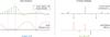 |
Fig. 2 Sparse recovery with annihilating filter method. The annihilation equation that the sparse signal should satisfy x(t)μ(t) = 0 is equivalent to a set of discrete convolution equations between uniformly sinusoidal samples and a finite length discrete filter in the Fourier domain. The mask function μ(t), which can be estimated from the given lowpass filtered samples of x(t), vanishes at the position where x(t) is different from zero. |
In a modern radio telescope, the number of antennas can be enormous (e.g., around 20 000 dipole antennas in LOFAR). In that case, it becomes unrealistic to send all raw data collected by the antenna arrays to a centralized correlator and obtain visibility measurements for each antenna pair. One commonly used strategy for data compression involves grouping antennas as stations and applying beamforming to antenna signals within each station. The visibility measurements are then obtained by taking the cross-correlations at the station level. Specifically, the beamformed visibility measurement from two stations (i,j) are:  (2)Here, L is the total number of stations, Q is the number of antennas per station;
  is the normalized baseline for the pair formed by the pth antenna in station i and the qth antenna in station j; and
  are beamforming weights. A typical beamforming strategy is matched beamforming, which amounts to choosing
  with r0 the focus direction of the matched beamforming (e.g., the zenith).
When digital beamforming is performed, either the beamshapes at each station must be accounted for – rendering the conventional imaging pipeline more computationally intensive – or neglected with potentially strong consequences for image accuracy (Tasse et al. 2013). The latter is the strategy most commonly employed in off-the-shelf CLEAN implementations (Offringa et al. 2014). In contrast, as we will show in Sect. 2.3, the proposed approach readily accounts for the beamformed visibilities with minimal effort.
In summary, LEAP can transparently work with either measurement Eq. (1)(without beamforming), or (2)(factoring in beamforming). To this end, we estimate the Fourier transform of the sky image on a (resolution-independent) uniform grid (e.g., 55 × 55 in a typical setup for radioastronomy) from the visibility measurements (2). The point source locations and amplitudes are subsequently obtained from these uniform Fourier transform reconstructions with the FRI sampling technique, which we review now in the next section.
2.2. Continuous domain sparse recovery with FRI sampling
In this section, we review a continuous-domain sparse recovery technique on both the methodology (Sect. 2.2.1) and the reconstruction algorithm aspects (Sect. 2.2.2). This technique will be adapted to solve point source estimation in radio astronomy in the next section (Sect. 2.3).
2.2.1. The classic FRI sampling framework
Sampling signals with finite rate of innovation (FRI; Vetterli et al. 2002; Blu et al. 2008) is a sampling theory for continuous-domain sparse signals. Typically, these signals have finite degrees of freedom (i.e., signal innovation) per unit time/space. The goal of FRI sampling is to estimate the finite number of unknown signal parameters from samples, or in general measurements, of the original continuous-domain sparse signal. A classic example of FRI signals, and the one most closely related to point source reconstruction in radio astronomy, is a τ-periodic Dirac stream (Vetterli et al. 2002):  (3)Within each period, there are K Dirac deltas with amplitudes αk located at tk. The objective is to reconstruct these 2K unknown parameters from samples of the sparse signal x(t).
Instead of directly reconstructing the original continuous-domain sparse signal x(t), FRI-based sparse recovery estimates a smooth “mask” function μ(t), typically a polynomial, which vanishes precisely at the non-zero locations of the sparse signal (Fig. 2). If we could find such a continuous function satisfying the annihilation equation μ(t)x(t) = 0, then the non-zero locations of the sparse signal are given by the roots of μ(t). The estimation of the amplitude for each non-zero element in x(t) is a linear problem, and can be easily solved once we have the non-zero locations of the sparse signal.
It remains to examine how the annihilation constraint μ(t)x(t) = 0 can be enforced algorithmically. A common feature of FRI signals is that they consist of, or can be transformed into, a weighted sum of sinusoids whose frequencies are related to the unknown parameters of the original continuous sparse signals. Thanks to a result first discovered more than two centuries ago (Prony 1795), we know that there exists a finite length discrete filter such that its convolution with uniformly sampled sinusoids is zero (hence the name “annihilating filter”). Consequently, we can enforce the continuous-domain annihilation constraint with a few discrete convolution equations.
Take the Dirac reconstruction (3)as an example. On the one hand, the given measurements are typically low-pass filtered samples of x(t), which have a direct correspondence to its Fourier series coefficients. On the other hand, the Fourier series coefficients are a sum of sinusoids uk:  (4)whose frequencies have a direct correspondence with the Dirac locations tk. By choosing a (K + 1)-tap filter [h0,...,hK] with z-transform
 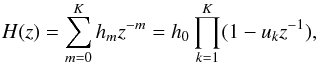 (5)then
  for all m. In the time domain, the Fourier domain convolution equations reduces to a multiplication between the sparse signal x(t) and a mask function
  , which vanishes at t = tk:
  (6)Readers are referred to Vetterli et al. (2002), Blu et al. (2008) for rigorous derivations of the annihilation equations.
Given sufficient measurements, the annihilating filter coefficients can be reconstructed from the annihilation equations. The Dirac locations are then obtained by taking the roots of the polynomial (5). Once we have tk, the amplitudes associated to each Dirac can be obtained by solving a simple least square estimation based on (4). It has been shown that a stream of K Dirac deltas can be perfectly recovered from at least 2K + 1 ideal (noise-free) samples (Vetterli et al. 2002).
2.2.2. Generalization to arbitrary measurements
The direct reconstruction based on the annihilation equations are sensitive to noise. Various algorithms have thus been proposed to improve the robustness of FRI reconstruction, including total least square minimization (Vetterli et al. 2002), Cadzow’s method (Blu et al. 2008), the matrix pencil approach (Urigüen et al. 2013), and structured low-rank approximation (Condat & Hirabayashi 2015). However, these approaches are designed to operate only on uniformly sampled measurements.
Recent work by Pan et al. (2017b) generalizes the classic FRI framework to cases with non-uniform samples making it applicable to point source reconstruction in radio astronomy. There, generic FRI reconstruction is recast as an approximation problem, where one would like to recover an FRI signal consistent with the given measurements. The re-synthesized measurements (based on the reconstructed FRI signal) should match the given (noisy) measurements up to the noise level. A valid solution to the approximation problem is obtained with the help of a constrained optimization, where the fitting error (e.g., the ℓ2 norm of the discrepancies) is minimized subject to the annihilation constraint: 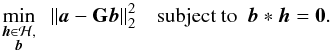 (7)Here
-
a is the given measurements of the sparse signal;
-
h is the annihilating filter coefficients, which belongs to a certain feasible set ℋ, e.g.,
 ;
; -
b is a set of (unknown) uniformly sampled sinusoids, which needs to be tailored to each specific sparse reconstruction problem;
-
G is a linear mapping from these uniform sinusoidal samples to the measurements.
More concretely, for the periodic stream of Dirac reconstruction in the previous section, we could take the ideally lowpass filtered samples as the measurements a, the Fourier series coefficients  as the uniform sinusoidal samples b, and the inverse discrete Fourier transform (DFT) as the linear mapping G (see (2.3.1) for cases of point source estimation in radio astronomy).
The sinusoidal samples b have to be taken on a uniform grid in order to apply the annihilation constraint. However, the grid step-size is flexible and is unrelated to the final resolution that can be achieved with FRI reconstruction, which is only related to the noise level (or in general the level of model mismatch). Experimentally, FRI-based sparse recovery reaches a lower bound, typically characterized by Cramér-Rao bound (Pan et al. 2017b). We define precisely the problem formulation in the case of radio interferometer point source reconstruction in the next section.
An efficient algorithm (Pan et al. 2017b) was proposed to solve (7)iteratively, where an ℓ × ℓ linear system of equations was solved at each iteration for a set of uniform sinusoidal samples b of size ℓ. The simplicity of the algorithm is beneficial for point source reconstructions in radio interferometer imaging. The recovery estimates point sources in the continuous domain directly from visibilities, and the complexity depends only on the dimension of b (typically around a few thousand). In terms of computational complexity, solving a dimension ℓ linear system of equations is at most  (see Golub & Van Loan 2012, Chap. 3). In contrast, CLEAN or compressed sensing based approaches have to estimate an intermediate sky image defined on a grid first before applying local peak detections in order to identify point sources. Consequently, the complexity of these algorithms is related to the size of the discrete image (around one million pixels or more), which is significantly larger than the dimension of the uniform sinusoidal samples b in a typical setup (see Sect. 3.5 for a concrete example).
Although the focus in this paper is on point source reconstructions, the FRI-based approach can also deal with extended source recovery. Given a suitable set of bases in which the extended sources have a sparse representation, the same algorithm can be applied in the transformation domain. However, substantially more work would be required to design a continuous domain “sparsifying” transformation for celestial sources (see Starck et al. 2010, for examples in a discrete setup), and hence this is left for future work.
2.3. Algorithm
In the previous section, we reviewed the generic form of an FRI-based sparse reconstruction. In this section, we adapt this continuous-domain sparse recovery framework to point source reconstructions in radio astronomy. The FRI-based approach estimates source locations first (Sect. 2.3.1) before solving a least square minimization for the source intensities (Sect. 2.3.2). A multi-band formulation, which may potentially reduce the amount of data needed significantly, are proposed in Sect. 2.3.3. Finally, an iterative strategy to refine the source estimation based on the current reconstruction is discussed in Sect. 2.3.4.
2.3.1. Estimation of point source locations
For point source reconstruction, the sky image consists of a sum of Dirac deltas:  (8)The goal is to reconstruct the source locations rk and intensities αk> 0 from the beamformed visibility measurements1:
 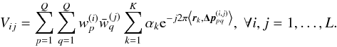 (9)The intensities of sources falling outside the telescope primary beam are significantly attenuated, hence it is reasonable to assume the sky image has finite spatial support, e.g.2rk ∈ [−τ1/ 2,τ1/ 2] × [−τ2/ 2,τ2/ 2]. The Fourier transform of the sky image, then can be represented by sinc interpolation3:
 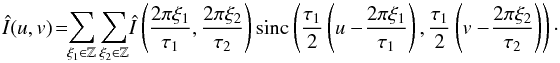 (10)From the FRI reconstruction perspective, as long as we can estimate both the uniformly sampled sinusoids Î(2πξ1/τ1,2πξ2/τ2) and the annihilating filter, then the source locations are given by finding roots of polynomials, whose coefficients are specified by the annihilating filters. In general, the zero-crossing of a 2D polynomial is a curve – any Dirac deltas that are located on the curve satisfy the annihilation constraints (Pan et al. 2014). In order to uniquely determine the Dirac locations, it is necessary to find two annihilating filters: the Dirac locations are then obtained from the intersections of the two associated curves (Pan et al. 2017a). Once the source locations are reconstructed, it is a linear problem to estimate source intensities, which amounts to solving a simple least square minimization (see details in Sect. 2.3.2).
However, this would require the estimation of infinitely many sinusoidal samples from a finite number of visibility measurements. One way to address this challenge is to assume additionally that the Fourier transform Î(u,v) is periodic with period 2πM × 2πN for some M and N such that Mτ1 and Nτ2 are odd numbers4. From Poisson sum formula, the Fourier transform of the sky image can be approximated as (see Pan et al. 2017b, for a similar treatment in 1D): 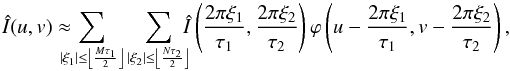 (11)where
  .
.
The beamformed visibility measurements (9)are linear combinations of irregularly sampled Fourier transform of the sky image at frequencies specified by the baselines of the antenna pairs  . Equation (11)provides a linear connection between a finite set of uniform sinusoidal samples Î(2πξ1/τ1,2πξ2/τ2) and these non-uniformly sampled Fourier transform. In terms of FRI sparse recovery, this amounts to solving a constrained minimization:
 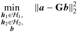 (12)subject to b ∗ h1 = 0andb ∗ h2 = 0,where
-
a is the visibility measurements (9);
-
b is the Fourier transform of the sky image on a uniform grid Î(2πξ1/τ1,2πξ2/τ2);
-
G is the linear mapping from the uniformly sampled Fourier transform b to the visibilities based on (9)and (11);
-
h1and h2 are two annihilating filters, each belonging to a certain feasible set, e.g.,
 ,
,  .
.
Similar to the 1D case, each annihilating filter defines a mask function in the spatial domain, whose value vanishes on a certain curve. The source locations are then given by the intersections of the two curves. In spatial domain, the annihilation constraints can be considered as requiring the multiplication between the two mask functions with the sky image (that contains a few point sources) be zero. Note that, instead of enforcing the reconstructed signal to follow the interpolation Eq. (11)exactly, we use it only as a metric to gauge the reconstruction quality in Eq. (2.3.1). This explains why a reasonably robust reconstruction is observed experimentally even when the periodicity assumption is violated (Pan et al. 2017b). However, see Sect. 2.3.4 for a strategy to refine the linear mapping based on the reconstructed source model.
2.3.2. Estimation of point source intensities
The source intensity αk are estimated by solving a least-square fitting problem based on the measurement Eq. (9)once we have reconstructed the source locations rk: ![Mathematical equation: \begin{eqnarray} \balpha^{\text{opt}}&=&\arg\min_{\balpha\in\R^K}\sum_{i,j=1}^L \left[V_{ij}-\sum_{p,q=1}^Q w_p^{(i)} \bar{w}_{q}^{(j)} \sum_{k=1}^K \alpha_k \e^{-j 2\pi \left\langle \br_k, \bDeltap^{(i,j)}_{pq} \right\rangle }\right]^2\!. \label{eq:opt_sources_intensities} \end{eqnarray}](/articles/aa/full_html/2017/12/aa31828-17/aa31828-17-eq85.png) (13)Equation (13)can be re-written more compactly in matrix form. For this we need to introduce a few quantities:
(13)Equation (13)can be re-written more compactly in matrix form. For this we need to introduce a few quantities:
-
The visibility matrix Σ ∈ CL × L whose terms are given by (Σ)ij = Vij, for all i,j = 1,...,L.
-
The antenna steering matrix A ∈ CLQ × K defined by
![Mathematical equation: \begin{equation} \Aa=\left[ \begin{matrix} \bm{\rho}^{(1)}(\br_1) &\ldots& \bm{\rho}^{(1)}(\br_K)\\ \bm{\rho}^{(2)}(\br_1) &\ldots &\bm{\rho}^{(2)}(\br_K)\\ \vdots &\vdots & \vdots\\ \bm{\rho}^{(L)}(\br_1) &\ldots &\bm{\rho}^{(L)}(\br_K) \end{matrix} \right], \end{equation}](/articles/aa/full_html/2017/12/aa31828-17/aa31828-17-eq90.png) (14)where
(14)where ![Mathematical equation: \hbox{$\bm{\rho}^{(i)}(\br_k)= \Big[ \e^{-j2\pi \langle\br_k,\bm{p}^{(i)}_1\rangle},\ldots,\e^{-j2\pi \langle\br_k,\bm{p}^{(i)}_Q\rangle} \Big] \in\mathbb{C}^Q$}](/articles/aa/full_html/2017/12/aa31828-17/aa31828-17-eq91.png) is the antenna steering vector for station i and rk are the reconstructed source locations.
is the antenna steering vector for station i and rk are the reconstructed source locations. -
the beamforming matrix
 is a block-diagonal matrix defined by
 ![Mathematical equation: \begin{equation} \bcW=\left[ \begin{matrix} \bar{\bm{w}}^{(1)} &\ldots&\bzero\\ \vdots & \ddots&\vdots\\ \bzero&\ldots &\bar{\bm{w}}^{(L)} \end{matrix} \right], \label{eq:beamformingMatrix} \end{equation}](/articles/aa/full_html/2017/12/aa31828-17/aa31828-17-eq93.png) (15)where
(15)where ![Mathematical equation: \hbox{$\bm{w}^{(i)}=\left[w_1^{(i)},\ldots,w_Q^{(i)}\right]\in\mathbb{C}^Q$}](/articles/aa/full_html/2017/12/aa31828-17/aa31828-17-eq94.png) is the beamforming vector for station i.
is the beamforming vector for station i.
With the notation introduced above, (13)reduces to: ![Mathematical equation: \begin{eqnarray} \balpha^{\text{opt}} &=&\arg\min_{\balpha\in\R^K} \left\| {\bf\rm \Sigma} - \bcW^\text{H} \Aa\,\diag(\bm{\alpha})\, \Aa^\text{H}\bcW \right\|_2^2\\ &=&\arg\min_{\balpha\in\R^K} \left\|\bm{\sigma}- \left[\left(\bcW^\text{T}\bar{\Aa}\right)\circ \left(\bcW^\text{H} \Aa\right) \right]\,\balpha \right\|_2^2, \label{eq:opt_standard_form} \end{eqnarray}](/articles/aa/full_html/2017/12/aa31828-17/aa31828-17-eq95.png) where
where  is the vectorization of the visibility matrix, and ° denotes the Khatri-Rao product (see van der Veen & Wijnholds 2013, for more details). The closed-form solution of (17) is
 ![Mathematical equation: \begin{equation} \balpha^{\text{opt}}=\left[ \left(\bcW^\text{T}\bar{\Aa}\right) \circ \left(\bcW^\text{H}\Aa\right) \right]^{\dagger} \,\bm{\sigma}, \end{equation}](/articles/aa/full_html/2017/12/aa31828-17/aa31828-17-eq98.png) (18)where † denotes the Moore-Penrose pseudo-inverse. The optimization problem (17)could be further constrained by α> 0 (since source intensities are positive) leading to a non-negative least-squares problem, which can be solved within a finite number of iterations (Lawson & Hanson 1995). Finally, when the number of sources is uncertain, a sparsity promoting penalty term ν ∥ α ∥ 1 could also be envisaged, with the parameter ν acting as model selection parameter. Unfortunately, such a penalty term would bias the estimation of the source intensities. Instead, we propose an alternative model order selection procedure, based on the fitting error (see Sect. 3.4).
(18)where † denotes the Moore-Penrose pseudo-inverse. The optimization problem (17)could be further constrained by α> 0 (since source intensities are positive) leading to a non-negative least-squares problem, which can be solved within a finite number of iterations (Lawson & Hanson 1995). Finally, when the number of sources is uncertain, a sparsity promoting penalty term ν ∥ α ∥ 1 could also be envisaged, with the parameter ν acting as model selection parameter. Unfortunately, such a penalty term would bias the estimation of the source intensities. Instead, we propose an alternative model order selection procedure, based on the fitting error (see Sect. 3.4).
2.3.3. Coherent multiband reconstruction
Modern radio telescopes operate over a wide frequency range, e.g., 30 MHz to 240 MHz for LOFAR (Van Haarlem et al. 2013). The emitted electromagnetic waves of celestial sources within the operation range are measured simultaneously, which are subsequently filtered into different sub-bands. If the consistency of the measurements across different sub-bands is exploited, it may potentially reduce significantly the integration times needed in order to have a reliable reconstruction.
Classic approaches, e.g., multi-frequency synthesis (Conway et al. 1990), and multi-frequency CLEAN (Sault & Wieringa 1994), try to map multi-frequency visibility measurements into a single sub-band centered at a reference frequency based on a frequency-dependent sky brightness distribution model.
With FRI-based sparse recovery, the mutual information shared across different sub-bands can be exploited in a coherent manner. It is usually reasonable to assume that the source locations remain the same across all subsequent sub-bands. Since the annihilating filter is uniquely specified by the point source locations alone, this implies that we should find one annihilating filter for all sub-bands such that the annihilation equations are satisfied5. In general, the source intensities αk differ from sub-band to sub-band. Hence, the uniformly sampled sinusoids, which are chosen as the interpolation knots Î(2πξ1/τ1,2πξ2/τ2) in Eq. (11), are sub-band-dependent. Then, the multiband point source reconstruction amounts to solving 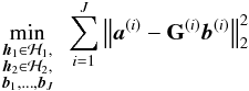 (19)subject to b(i) ∗ h1 = 0andb(i) ∗ h2 = 0 fori = 1,··· ,J,
where a(i) and b(i) are the visibility measurements and the uniform sinusoidal samples in the ith sub-band, respectively; and G(i) is the linear mapping based on Eqs. (9)and (11)for each one of the J sub-bands. Note that (19)is in fact the same formulation6 as Eq. (2.3.1) with a change of variables: ![Mathematical equation: \begin{equation} \ba=\left[ \begin{matrix} \ba^{(1)}\\\vdots\\\ba^{(J)} \end{matrix} \right], \bb=\left[ \begin{matrix} \bb^{(1)}\\\vdots\\\bb^{(J)} \end{matrix} \right], \text{ and } \GG = \left[ \begin{matrix} \GG^{(1)} & \ldots & \bzero\\ \vdots& \ddots &\vdots \\ \bzero & \ldots & \GG^{(J)} \end{matrix} \right]. \end{equation}](/articles/aa/full_html/2017/12/aa31828-17/aa31828-17-eq112.png) (20)Once we have estimated the common annihilating filter h for all sub-bands, the source locations and intensities are determined in the same manner as in the single band case.
(20)Once we have estimated the common annihilating filter h for all sub-bands, the source locations and intensities are determined in the same manner as in the single band case.
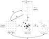 |
Fig. 3 Diagram of the various linear operators involved in the update strategy for the forward operator G (see details in Sects. 2.3.1 and 2.3.4). |
2.3.4. Update strategy for the linear mapping G in Eq. (2.3.1)
Ideally, G should be constructed based on the measurement Eq. (9)in the constrained optimization Eq. (2.3.1), and the discrepancies between the re-synthesized visibilities Gb with the given measurements minimized. If the actual mapping, which links the Fourier transform of the sky image on a uniform grid to the visibility measurement, were available, then the FRI-based sparse recovery would give the exact reconstruction from the noiseless measurements.However, this is not feasible, as the exact mapping based on Eq. (9)contains the source locations and intensities, which are unknown a priori. One possible strategy is to use the initial reconstruction, where G was approximated with the periodic-sinc interpolation Eq. (11), to update the objective function in Eq. (2.3.1).
To describe this update strategy, we need to introduce some notation (see Fig. 3 for a summary):
-
Denote by G0 the linear operator that maps source intensities α to the Fourier transform of the sky image on a uniform grid (u,v) = (2πξ1/τ1,2πξ2/τ2) as in Eq. (11):
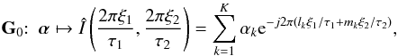 (21)with some given source locations rk = (lk,mk).
 Denote by G1 the matrix mapping the source intensities α to the non-gridded Fourier samples
 :
:  (22)The matrix G1 can also be expressed of the antenna steering matrix A as
Denote by W ∈ CL2 × L2Q2 the cross-beamforming matrix that beamforms the off-grid Fourier samples:
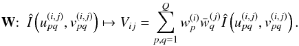 (23)Here W is related to the beamforming matrix
  in (15)as:
Finally, denote by Φ the periodic-sinc interpolation (11)evaluated at non-gridded Fourier samples
 :
: 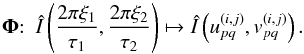 (24)
(24)
 , where
  is the Moore-Penrose pseudo-inverse
  .
.
Note that  , which transforms the uniformly sampled Fourier data to the irregularly sampled ones7, has a rank at most K. At any intermediate step, we may choose the linear mapping G as:
  where G0 and G1 are built with the reconstructed point source locations and
  is the orthogonal projection onto the null space of :
  Experimentally, such an iterative strategy manages to refine the linear mapping and results in a reliable reconstruction (see an example in Sect. 3.2).
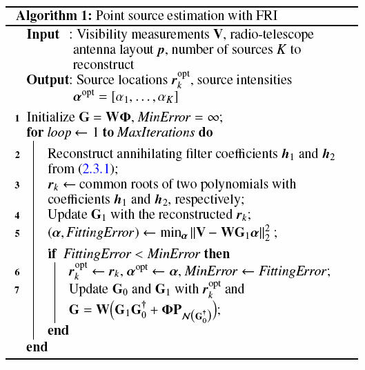
We emphasize that the reconstruction quality should always be measured based on Eq. (9), with rk and αk the reconstructed source locations and intensities, respectively, regardless of the update strategy for the linear mapping G. We summarize the FRI-based point source reconstruction in Algorithm 1.
Summary of various datasets used in the experiments.
3. Results
3.1. Data and experiment setup
The proposed FRI-based sparse recovery approach for point source estimation (LEAP) was validated with both simulated visibilities and real observations from LOFAR. In simulation, visibilities were generated from ground truth point source parameters (locations and intensities) with the LOFAR core station antenna layout. In experiments with real LOFAR observations, we sub-sampled the visibility measurements over different integration times such that only 2% or 0.25% of the total integration times in the measurement set were available to the reconstruction algorithms in single band and multi-band scenarios, respectively.
We should point out that it is not only the number of integration times that matters: with the same number of integration times taken consecutively, a much worse reconstruction is obtained by both CLEAN and LEAP. Experimentally, we observe that it is better to take measurements that are well-spread over the whole acquisition time. One explain might be that with a larger time separation between adjacent measurements, the earth has more significant displacement in space. Thus, it allows the radio interferometer to sample the (u,v)-plane sparsely but over a large area (instead of densely sampling a local area as in the case with consecutive integration times). Spatial diversity in the (u,v) domain sampling makes the reconstruction algorithms more resilient to noise.
We summarize the experimental setups in terms of antenna layouts, integration time and sub-band selections in Table 1. The reconstruction quality of the FRI-based approach was measured by the average distance8 between the recovered and the ground truth source locations (in simulation) or the catalog data (in real-data experiments).
The LEAP results were compared to those obtained from WSClean9, which implements the state-of-the-art w-stacking CLEAN algorithm (Offringa et al. 2014). The maximum number of iterations for the WSClean algorithm was set to 4 × 10⁴. The threshold level was determined automatically by the WSClean algorithm based on the estimated background noise level. Unlike LEAP, which reconstructs point source locations and intensities directly, the CLEAN algorithm typically produces discrete sky images, which will be compared to the FRI reconstruction by visual inspection.
In the following part, we first conduct simulations to verify the effectiveness of the updating strategy of the linear mapping in Sect. 3.2. Next, we investigate the resolvability of the proposed algorithm by simulating visibilities from two point sources that are separated by various distances in Sect. 3.3. Further, a strategy to avoid false detections by selecting an adequate model order is validated through simulations in Sect. 3.4. Finally, we apply LEAP to actual LOFAR observations from the Boötes field (Sect. 3.5), which consists of mostly point sources; and the “Toothbrush” cluster (Sect. 3.6), which has an extended structure in addition to many point sources within the field of view.
3.2. Iterative refinement of linear mapping
One challenge in applying the FRI-based sparse recovery technique to radio astronomy is identifying a suitable surrogate function to gauge reconstruction quality – the ideal MSE criteria based on the measurement Eq. (9)requires the knowledge of the (unknown) ground truth source locations and intensities. We proposed one possible strategy that allows us to refine the objective function based on the current reconstruction in Sect. 2.3.4. In order to verify the effectiveness of such a strategy, we generated an empty measurement set (MS) with the LOFAR antenna layout as specified in Table 1 Dataset I. The MS file is then filled with noiseless visibilities that are simulated based on (9)from two point sources with randomly generated intensities and locations within the field-of-view (5° × 5°).
The evolution of the fitting error between the re-synthesized visibilities (9)(based on the reconstructed point source parameters) and the given visibility measurements is shown in Fig. 4. The reconstructed sources are included for visual comparison, where the dirty image is overlaid with the reconstructed and ground truth point sources. With this simple updating strategy, we indeed obtain the exact reconstruction after a few iterations.
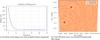 |
Fig. 4 Iterative refinement of the linear mapping G in (2.3.1) for exact point source reconstruction (see details in Sect. 2.3.4). Panel a: The evolution of the fitting error between the re-synthesized and given noiseless visibility measurements. Panel b: Exact reconstruction of the point sources with LEAP (background image: dirty image from the same visibility measurements). |
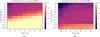 |
Fig. 5 Average reconstruction success rate (25) of two point sources that are separated by various distances from noisy visibility measurements with a) LEAP and b) CLEAN. The reconstructed point sources with CLEAN are extracted from the corresponding CLEAN model image. A point source is considered to be successfully reconstructed if the estimated source location is within half the separation distance with the ground truth source location. Results for each noise level and source separation are averaged over 100 different signal and noise realizations. Instrument angular resolution is 4′49.2′′. |
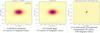 |
Fig. 6 Resolve closely located sources accurately with LEAP (S/N = 20 dB, source separation: 1′30′′, antenna layout: 24 LOFAR core stations, background: CLEAN image). Panel a: LEAP reconstruction. Panel b: CLEAN image from the same set of visibility measurements. Panel c: CLEAN image from additional visibilities with higher time resolution (8.01 s between adjacent integration times) and longer baselines (56 LOFAR core and remote stations). The setup in (c) with longer baselines reduces the telescope angular resolution to 6.10′′. |
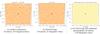 |
Fig. 7 Reliable estimation of sources from highly noisy measurements with LEAP (S/N = −10 dB, source separation: 1°30′, antenna layout: 24 LOFAR core stations, background: CLEAN image). Panel a: LEAP reconstruction. Panel b: CLEAN image from the same set of visibility measurements. Panel c: CLEAN image from additional visibilities with higher time resolution (8.01 s between adjacent integration times) from 24 core stations. |
3.3. Source resolution
In this section, we investigate the resolving power of the proposed FRI-based sparse recovery, by comparing the performance to that of CLEAN. The antenna layout of the 24 LOFAR core stations was used to simulate a 7 h single sub-band observation with center frequency 145.8 MHz (HBA band). The visibility measurements were taken every 400.56 s, leading to a total 63 sets of visibilities at different time instances. The maximum baseline was 713.3 wavelengths, which corresponds to an instrument angular resolution of 4′49.2′′. For simplicity, we did not account for polarization effects in this work. We note, however, that the technique described in Sect. 2.3.3 to reconstruct point sources from multi-bands may be adapted to treat together different polarizations in a coherent manner (see remarks in footnote 5).
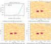 |
Fig. 8 Model order selection based on the fitting error of the reconstructed point source model and the given visibility measurements (Dataset I). The model order is the minimum number of sources such that the fitting error reaches the noise level of the measurements (Background images of (b)–(d): CLEAN images; signal to noise ratio (S/N) in the visibilities: 0 dB; Actual model order: 3). Panel a: Evolution of the fitting errors against different point source model orders K in (8). Panel b: Reconstructed source models with the correct model order K = 3. Panel c: Reconstruction with under-estimated model order K = 1. Panel d: Reconstruction with over-estimated model order K = 5. |
We simulated visibilities of two point sources with unitary intensities. The two sources were separated by distances varying from 10′′ to 10′ on a log scale. The particular antenna layout means there is not always the same sensitivity along all directions. To alleviate this potential direction-dependent bias, we averaged the results over 100 signal realizations with different relative orientations between the two sources for each separation distance. Circularly symmetric complex Gaussian white noise is added to the noiseless visibilities such that the signal to noise ratio (S/N) in the visibility measurements ranges from −10 dB to 20 dB with a step size of 5 dB.
A point source was considered to be successfully reconstructed if the estimated source location is within half the separation distance between the two sources, from the ground truth source location. Hence, the average reconstruction success rate for K point sources is:  (25)Here dist(·,·) computes the distance between the reconstructed
  and ground truth source locations rk; and Δr is the separation between the two sources. We extracted the reconstructed source locations from the CLEAN model image with a pixel size 3.5′′. The average reconstruction success rate is shown in Fig. 5 for both CLEAN and LEAP.
Note that while the instrument angular resolution was close to 5′ here, the FRI-based sparse recovery still manages to resolve two sources beyond the instrument limitation in many cases. This is in stark contrast to image-based approaches such as CLEAN or compressed sensing (CS), where the reconstructions are typically spatial domain images – in order to determine point source locations (and intensities), an additional blob detection algorithm needs to be employed. In contrast, the FRI-based approach starts from a point source assumption, and reconstructs the source parameters directly without going through an intermediate spatial domain image.
To better illustrate the difference between the proposed method and other image-based reconstruction methods, we include two examples where it would otherwise not be possible to recover all point sources based on the estimated sky images (Figs. 6 and 7):
-
Figure 6 shows how two closely located sources,1′30′′ apart, are accurately estimated from mildly noisy visibility measurements (S/N = 20 dB) with LEAP, while the CLEAN image contains one big blob encompassing both sources. In fact, neither one of the two source locations corresponds to the peak of the blob. Further, we considered another case for CLEAN, where additional measurements from 32 LOFAR remote stations were added. With this configuration, the telescope has a much smaller angular resolution 6.10′′ (compared with 4′49.2′′ with 24 LOFAR core stations only). The time resolution of the visibility measurements from all stations is also increased: adjacent integration times are separated by 8.01 s. In total, visibilities from all 56 stations at 3150 integration times are given to the CLEAN algorithm. The blob size is significantly reduced and both sources are resolved by CLEAN (Fig. 6c).
-
Figure 7 shows two well-separated sources, 1°30′ apart, are reliably reconstructed from highly noisy visibility measurements (S/N = −10 dB) with LEAP, while the weaker source, whose intensity is 1/5 of that of the strong source, is completely buried in the noisy background, and cannot be detected from the estimated sky image using CLEAN. With additional visibilities from a higher time resolution (8.01 s between adjacent integration times), both the strong source in the middle of the field of view and the weak source are correctly reconstructed by CLEAN (Fig. 7c).
3.4. Model order selection
The point source model requires a choice of a certain model order K. In simulation, this parameter is assumed to be given a priori, while with actual observations, we have to specify/estimate it. A strategy is then needed to determine if a particular choice of K over-estimates10 the model order and leads to false detections. One method is based on the fitting error between the reconstructed source model and the given measurements (Gilliam & Blu 2016). From our experience, the FRI reconstruction algorithm can reliably estimate a sparse signal that fits the given measurements up to the noise level (Pan et al. 2017b). The strategy is constructive since we can usually estimate the noise level from a source finding algorithm, e.g., Duchamp (Whiting 2012), SoFiA (Serra et al. 2015), and PyBDSF11, or manually specify the approximation error allowed in the reconstruction.
In particular, if the fitting error achieved by FRI-based reconstruction is still within the noise level with a lower model order, then we can further reduce the number of sources by one. The final model order is obtained by repeating the process until any further reduction in K leads to a fitting error above the noise level.
We validated this approach by simulating visibility measurements for K = 3 point sources from 24 LOFAR core stations (Dataset I in Table 1). The noiseless visibilities are contaminated by circularly symmetric complex Gaussian white noise such that the S/N in the visibility measurements is 0 dB. We applied LEAP with different model orders, and compared the noise level with the fitting errors between the given and the re-synthesized visibility measurements based on (9)(Fig. 8a). As soon as the model order is reduced below the actual number of sources, the fitting error jumps above the noise level, while this error remains stable for over-estimation cases. The reconstructed point source model that corresponds to under-estimation and over-estimation cases are also included in Fig. 8.
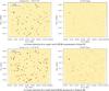 |
Fig. 9 Source detection from actual LOFAR observations from the Boötes field (Dataset II and III) with LEAP (the left column) and CLEAN (the right column). Panel a: LEAP and CLEAN reconstruction from single band visibility measurements at frequency 145.8 MHz with 72 integration times. Panel b: LEAP and CLEAN reconstruction from visibility measurements within 8 sub-bands at frequencies from 145.8 MHz to 146.5 MHz with 9 integration times. |
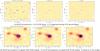 |
Fig. 10 Point source reconstruction from actual LOFAR observations from the Toothbrush cluster RX J0603.3+4214 (Dataset IV). Point sources are reliably estimated even in the presence of extended sources (the Toothbrush cluster). Existence of sources are validated by referencing both the TGSS and the NVSS catalog. Panel a: The reconstructed point sources with LEAP. Panel b: The CLEAN image from the same set of visibility measurements. Panel c: The deconvoluted image with a compressed sensing (CS) based approach (Dabbech et al. 2015). Zoom-in comparisons of the LEAP reconstruction against d) the TGSS catalog and e) the NVSS catalog around the Toothbrush cluster. Panel f: Zoom-in plot of the CS reconstruction around the toothbrush cluster. |
3.5. Actual LOFAR observation: Boötes field
In the previous section, we validated the robustness of the proposed FRI-based sparse recovery method with simulated point sources. In this section, we apply LEAP to an actual LOFAR observation from the Boötes field. Source estimation from real observations of a radio telescope presents a significant challenge over and above ideal simulation conditions. Visibility measurements in a typical setting suffer from severe noise contamination, which may arise from thermal noise at antennas, the planar approximation (1), as well as directional dependent artifacts due to ionosphere variations (Williams et al. 2016). We used12 the visibility measurements from the 24 LOFAR core stations and 4 remote stations closest to the telescope center, and considered two different scenarios for the point source reconstruction in the Boötes field:
-
1.
Single-band visibility measurements at 145.8 MHz were extracted from the measurement set (MS). We sub-sampled the MS file uniformly every 50 integration times (~7 min), leading to a total 72 sets of visibilities from 2% of the all integration times. See Sects. 2.3.1 and 2.3.2 for the algorithmic details.
-
2.
Visibility measurements within 8 sub-bands centered at frequencies from 145.8 MHz to 146.5 MHz were extracted from the MS file. In total, 9 sets of visibilities at different integration times were given to the reconstruction algorithms by sub-sampling the MS file every 400 integration times (~53 min). Sources were reconstructed with the multi-band formulation presented in Sect. 2.3.3.
In both cases, LEAP reconstructed Fourier transform of the sky image within each frequency sub-band, on a uniform grid of size 57 × 63 that spanned the telescope uv-coverage. The source locations were subsequently estimated from these uniform Fourier data. We fixed a priori the number of sources to be K = 100 in Eq. (8)for the LEAP reconstruction. Of course, in practice an non-arbitrary choice of an adequate model order K is needed, and this is discussed in Sect. 3.4.
The reconstructed point sources for the single-band and multi-band cases are plotted in Fig. 9, where the background image is the corresponding CLEAN image reconstructed from the same sets of visibility measurements in each case. We compare the estimated source parameters with a catalog of the Boötes field at 130 ~ 169 MHz (Williams et al. 2016). The errors of the estimated source locations are 1′17.79′′ and 1′38.01′′ in the single-band and multi-band cases, respectively. Similar to the observations in simulated cases, we find that LEAP can reliably resolve closely located sources from the actual LOFAR measurements. The advantage of the FRI-based sparse recovery, which gives a direct estimate of the point source parameters, is evident by comparing the CLEAN image in both single-band and multi-band cases: several sources would otherwise be too weak to be reliably detected with a blob detection algorithm applied to the CLEAN image without introducing many false detections.
3.6. Acutal LOFAR observation: Toothbrush cluster
A natural question to ask is how well the algorithm recovers point sources in the presence of extended sources within the field of view. In order to test their influence, we applied LEAP to a LOFAR observation from the Toothbrush cluster RX J0603.3+4214, which contains one of the brightest radio relics. The toothbrush shape is suggested to be a consequence of a triple merger event based on simulation (Brüggen et al. 2012). We used the LOFAR observation with both the 24 core stations and 12 remote stations within a single-band at frequency 132.1 MHz (Dataset IV in Table 1).
The LEAP reconstruction results are compared to the CLEAN image. We also included the deconvolved image obtained with a compressed sensing (CS) based approach (Dabbech et al. 2015) for reference. We overlaid the CLEAN image with the reconstructed point sources from LEAP in Fig. 10, and validated the existence of sources by comparing the reconstructions with the 150MHz TIFR GMRT sky survey (TGSS; Intema et al. 2017). Even in the presence of the Toothbrush cluster at the center of the field of view, LEAP is robust enough to estimate the point sources reliably. The average reconstruction error of the source locations compared with the TGSS catalog is 2′43.60′′. A zoom-in plot, Fig. 10c, of the area around the toothbrush cluster, reveals that LEAP reconstructed a few sources not in the TGSS catalog (and hence are mismatched to other sources in the catalog). In order to determine whether theses sources were false detections, we cross-referenced with the NRAO VLA sky survey (NVSS; Condon et al. 1998), which observes the sky at a much higher frequency (1.4 GHz). The extra sources reconstructed by LEAP were indeed confirmed to be actual radio sources (Fig. 10d). The average LEAP reconstruction with respect to the NVSS catalog was 2′1.36′′.
4. Discussion
4.1. Resolution
In CLEAN-based source estimation algorithms, the reconstructed sky model (which consists of a few non-zero pixels around sources) are convolved with a point spread function (a.k.a. the “CLEAN beam”). The motivation for such an additional smoothing step is to reflect the angular resolution of a given instrument – the size of the CLEAN beam is determined by the diffraction limit imposed by the instrument with a given maximum baseline. Consequently, it is not possible to resolve sources beyond the instrument angular resolution. In practice, the minimum angular resolution that can be achieved by CLEAN is much larger than the instrument diffraction limit as noticed in Garsden et al. (2015). This is also observed in the two-source simulations in Sect. 3.3: within the simulation setup (which has a maximum source separation of 10′ and an instrument angular resolution 4′49.2′′), CLEAN cannot always resolve both sources consistently even for cases with relative large source separation and low noise levels.
In comparison, LEAP directly reconstructs the source locations in continuous space. The final resolution achievable is only related to the noise level in the visibility measurements. This is a direct consequence of enforcing continuous domain sparsity (i.e., the point source model) in the reconstruction process. LEAP tries to fit the given visibility measurements optimally (in the least square sense) with a point source model. From the experimental results in Figs. 5 and 6a, it indeed manages to resolve sources separated by a distance well below the instrument angular resolution. Further, experiments with actual LOFAR observations from the Boötes field and the Toothbrush cluster (Sects. 3.5 and 3.6, respectively) also confirm the ability of LEAP to identify closely located sources reliably.
4.2. Efficient use of visibility measurements
In the experiments with actual LOFAR observations, we sub-sampled13 the measurement set along different integration times: 2% and 0.25% of the total integration times is used in the single-band and the multi-band reconstruction respectively. Even with such little data, the point sources were estimated accurately by LEAP. This is potentially useful for a modern radio-interferometer like LOFAR or the next generation Square Kilometer Array (SKA), which consists of an array of numerous omnidirectional antennas. With an efficient algorithm, like LEAP, using only a fraction of the total observations can still yield reconstruction accuracy comparable to a conventional method (e.g., CLEAN) requiring significantly more integration times and longer baselines (e.g., Fig. 7). Another potential application of LEAP could be for the Very Long Baseline Interferometry (VLBI), which has sparse coverage in the uv domain.
5. Conclusions
We investigated the FRI-based continuous-domain sparse recovery framework in the challenging radio astronomy setting with both simulations and actual LOFAR observations, and demonstrated that the proposed approach (LEAP) can accurately resolve closely located sources under various noise conditions. In particular, we showed that it is possible to go beyond the instrument angular resolution. A comparable reconstruction accuracy to CLEAN can be achieved with significantly fewer measurements. Further, we developed a multi-band reconstruction scheme that estimates the point sources consistently among different sub-bands, and demonstrated the effectiveness of the multi-band reconstruction strategy given actual LOFAR observations. In order to facilitate the application of this new approach for source estimation in radio astronomy, the Python implementation is made available online14.
For future work, we will consider the potential application in calibration, where an accurate source estimation is essential for
subsequent imaging. Another interesting application could be for pulsar detection (from the antenna signals), given that LEAP can have reliable reconstructions even from very limited data. We will also extend the current framework to the sphere, to improve performance for instruments with a wide field-of-view, such as the Murchison Wide-field Array (MWA).
Without loss of generality, we can always shift the coordinates such that the telescope primary beam is centered at the origin.
In cases where strong sources fall outside the assumed spatial support and still have significant contributions to the visibility measurements, the interpolation representation here will be less accurate.
This is for the consideration of the convergence of Poisson sum equation (see Blu et al. 2008, for details).
The same approach can be applied to measurements of different polarizations within the same sub-band, where the source locations are common but intensities differ for each polarization.
To be precise, the convolution in the annihilation constraints in the multiband case should be understood as a convolution for each sub-band, which amounts to vertically stacking the convolution matrices associated with all sub-bands.
Superficially, this looks similar to the “gridding” in a conventional approach, e.g., CLEAN. However, unlike CLEAN, the final resolution that can be achieved by the FRI-based algorithm is not related to the grid step size but only the noise level in the given measurements (see Pan et al. 2017b).
The correspondence between the reconstructed and ground truth source locations were obtained by permuting the source locations such that the distance between the permuted reconstruction and the ground truth source locations was minimized.
Available at https://sourceforge.net/projects/wsclean/
In the case of under-estimation, the most dominating point sources will be reconstructed by the algorithm with a fitting error above the noise level (see an example in Fig. 8c).
Available at https://github.com/lofar-astron/PyBDSF
During the observation, 4 out of the 24 core stations were not working.
This is different than taking the measurements with same number of consecutive integration times. See our comments at the beginning of Sect. 3.1.
The Python package is available at https://github.com/hanjiepan/LEAP
Acknowledgments
We acknowledge the financial support from the Dutch Ministry of Economische Zaken, and the province of Drenthe as part of the collaboration between IBM and ASTRON in the DOME project; an ERC Advanced Grant – Support for Frontier Research – SPARSAM No. 247006; the Swiss National Science Foundation under Grant SNF–20FP-1_151073; and the Hong Kong Research Grant Council under the General Research Fund CUHK14200114. We gratefully thank Tammo Jan Dijkema from ASTRON for the LOFAR data from both the Boötes field and the Toothbrush cluster. We appreciate Sepand Kashani’s help in the data pre-processing of the measurement set.
References
- Bhatnagar, S., & Cornwell, T. 2004, A&A, 426, 747 [NASA ADS] [CrossRef] [EDP Sciences] [Google Scholar]
- Blu, T., Dragotti, P. L., Vetterli, M., Marziliano, P., & Coulot, L. 2008, IEEE Signal Process. Mag., 25, 31 [NASA ADS] [CrossRef] [Google Scholar]
- Brüggen, M., van Weeren, R., & Röttgering, H. 2012, MNRAS, 425, L76 [NASA ADS] [CrossRef] [Google Scholar]
- Carrillo, R. E., McEwen, J. D., & Wiaux, Y. 2014, MNRAS, 439, 3591 [NASA ADS] [CrossRef] [MathSciNet] [Google Scholar]
- Condat, L., & Hirabayashi, A. 2015, Sampl. Theory Signal Image Process., 14, 17 [Google Scholar]
- Condon, J., Cotton, W., Greisen, E., et al. 1998, AJ, 115, 1693 [NASA ADS] [CrossRef] [Google Scholar]
- Conway, J., Cornwell, T., & Wilkinson, P. 1990, MNRAS, 246, 490 [NASA ADS] [Google Scholar]
- Cornwell, T. J., Golap, K., & Bhatnagar, S. 2008, IEEE J. Sel. Top. Signal Process., 2, 647 [NASA ADS] [CrossRef] [Google Scholar]
- Dabbech, A., Ferrari, C., Mary, D., et al. 2015, A&A, 576, A7 [NASA ADS] [CrossRef] [EDP Sciences] [Google Scholar]
- Garsden, H., Girard, J., Starck, J.-L., et al. 2015, A&A, 575, A90 [NASA ADS] [CrossRef] [EDP Sciences] [Google Scholar]
- Gilliam, C., & Blu, T. 2016, in Proc. Forty-first IEEE International Conference on Acoustics, Speech, and Signal Processing (ICASSP’16), 4019 [Google Scholar]
- Golub, G. H., & Van Loan, C. F. 2012, Matrix Computations (Johns Hopkins University Press), 3 [Google Scholar]
- Högbom, J. 1974, A&AS, 15, 417 [Google Scholar]
- Intema, H., Jagannathan, P., Mooley, K., & Frail, D. 2017, A&A, 598, A78 [NASA ADS] [CrossRef] [EDP Sciences] [Google Scholar]
- Lawson, C. L., & Hanson, R. J. 1995, Solving Least Squares Problems (SIAM) [Google Scholar]
- Maravić, I., & Vetterli, M. 2005, IEEE Trans. Signal Process., 53, 2788 [NASA ADS] [CrossRef] [Google Scholar]
- Offringa, A., McKinley, B., Hurley-Walker, N., et al. 2014, MNRAS, 444, 606 [NASA ADS] [CrossRef] [Google Scholar]
- Ongie, G., & Jacob, M. 2016, SIAM J. Imaging Sci., 9, 1004 [CrossRef] [Google Scholar]
- Pan, H., Blu, T., & Dragotti, P. L. 2014, IEEE Trans. Signal Process., 62, 458 [NASA ADS] [CrossRef] [Google Scholar]
- Pan, H., Blu, T., & Vetterli, M. 2017a, IEEE Trans. Signal Process., submitted [Google Scholar]
- Pan, H., Blu, T., & Vetterli, M. 2017b, IEEE Trans. Signal Process., 65, 821 [NASA ADS] [CrossRef] [Google Scholar]
- Prony, R. 1795, J. Ecol. Polytech., 1, 24 [Google Scholar]
- Sault, R., & Wieringa, M. 1994, A&AS, 108 [Google Scholar]
- Schwab, F. 1984, Optimal Gridding of Visibility Data in Radio Interferometry (Cambridge University Press), 333 [Google Scholar]
- Serra, P., Westmeier, T., Giese, N., et al. 2015, MNRAS, 448, 1922 [NASA ADS] [CrossRef] [Google Scholar]
- Shukla, P., & Dragotti, P. L. 2007, IEEE Trans. Signal Process., 55, 3670 [NASA ADS] [CrossRef] [Google Scholar]
- Simeoni, M. M. J.-A. 2015, Towards more accurate and efficient beamformed radio interferometry imaging, Tech. Rep., École Polytechnique Fédérale de Lausanne [Google Scholar]
- Starck, J.-L., Murtagh, F., & Fadili, J. M. 2010, Sparse Image and Signal Processing: Wavelets, Curvelets, Morphological Diversity (Cambridge University Press) [Google Scholar]
- Tasse, C., van der Tol, S., van Zwieten, J., van Diepen, G., & Bhatnagar, S. 2013, A&A, 553, A105 [NASA ADS] [CrossRef] [EDP Sciences] [Google Scholar]
- Taylor, G. B., Carilli, C. L., & Perley, R. A. 1999, in Synthesis Imaging in Radio Astronomy II, 180 [Google Scholar]
- Thompson, A. R., Moran, J. M., & Swenson, G. W. 2001, Interferometry and Synthesis in Radio Astronomy (John Wiley & Sons) [Google Scholar]
- Urigüen, J., Blu, T., & Dragotti, P. L. 2013, IEEE Trans. Signal Process., 61, 5310 [NASA ADS] [CrossRef] [Google Scholar]
- van der Veen, A.-J., & Wijnholds, S. J. 2013, in Handbook of Signal Processing Systems (Springer), 421 [Google Scholar]
- Van Haarlem, M., Wise, M., Gunst, A., et al. 2013, A&A, 556, A2 [NASA ADS] [CrossRef] [EDP Sciences] [Google Scholar]
- Vetterli, M., Marziliano, P., & Blu, T. 2002, IEEE Trans. Signal Process., 50, 1417 [NASA ADS] [CrossRef] [Google Scholar]
- Whiting, M. T. 2012, MNRAS, 421, 3242 [NASA ADS] [CrossRef] [Google Scholar]
- Wiaux, Y., Puy, G., & Vandergheynst, P. 2010, MNRAS, 402, 2626 [NASA ADS] [CrossRef] [Google Scholar]
- Williams, W., Van Weeren, R., Röttgering, H., et al. 2016, MNRAS, 460, 2385 [NASA ADS] [CrossRef] [Google Scholar]
All Tables
All Figures
|
Fig. 1 Existing imaging algorithms estimate the locations and intensities of celestial sources on a uniform gird. In practice, sources do not line up so conveniently, and can fall off-grid. Gridding hence results in a less accurate estimation of the location estimations as well as a potential overestimation of intensities due to multiple sources being merged to the same pixel. |
| In the text | |
|
Fig. 2 Sparse recovery with annihilating filter method. The annihilation equation that the sparse signal should satisfy x(t)μ(t) = 0 is equivalent to a set of discrete convolution equations between uniformly sinusoidal samples and a finite length discrete filter in the Fourier domain. The mask function μ(t), which can be estimated from the given lowpass filtered samples of x(t), vanishes at the position where x(t) is different from zero. |
| In the text | |
|
Fig. 3 Diagram of the various linear operators involved in the update strategy for the forward operator G (see details in Sects. 2.3.1 and 2.3.4). |
| In the text | |
|
Fig. 4 Iterative refinement of the linear mapping G in (2.3.1) for exact point source reconstruction (see details in Sect. 2.3.4). Panel a: The evolution of the fitting error between the re-synthesized and given noiseless visibility measurements. Panel b: Exact reconstruction of the point sources with LEAP (background image: dirty image from the same visibility measurements). |
| In the text | |
|
Fig. 5 Average reconstruction success rate (25) of two point sources that are separated by various distances from noisy visibility measurements with a) LEAP and b) CLEAN. The reconstructed point sources with CLEAN are extracted from the corresponding CLEAN model image. A point source is considered to be successfully reconstructed if the estimated source location is within half the separation distance with the ground truth source location. Results for each noise level and source separation are averaged over 100 different signal and noise realizations. Instrument angular resolution is 4′49.2′′. |
| In the text | |
|
Fig. 6 Resolve closely located sources accurately with LEAP (S/N = 20 dB, source separation: 1′30′′, antenna layout: 24 LOFAR core stations, background: CLEAN image). Panel a: LEAP reconstruction. Panel b: CLEAN image from the same set of visibility measurements. Panel c: CLEAN image from additional visibilities with higher time resolution (8.01 s between adjacent integration times) and longer baselines (56 LOFAR core and remote stations). The setup in (c) with longer baselines reduces the telescope angular resolution to 6.10′′. |
| In the text | |
|
Fig. 7 Reliable estimation of sources from highly noisy measurements with LEAP (S/N = −10 dB, source separation: 1°30′, antenna layout: 24 LOFAR core stations, background: CLEAN image). Panel a: LEAP reconstruction. Panel b: CLEAN image from the same set of visibility measurements. Panel c: CLEAN image from additional visibilities with higher time resolution (8.01 s between adjacent integration times) from 24 core stations. |
| In the text | |
|
Fig. 8 Model order selection based on the fitting error of the reconstructed point source model and the given visibility measurements (Dataset I). The model order is the minimum number of sources such that the fitting error reaches the noise level of the measurements (Background images of (b)–(d): CLEAN images; signal to noise ratio (S/N) in the visibilities: 0 dB; Actual model order: 3). Panel a: Evolution of the fitting errors against different point source model orders K in (8). Panel b: Reconstructed source models with the correct model order K = 3. Panel c: Reconstruction with under-estimated model order K = 1. Panel d: Reconstruction with over-estimated model order K = 5. |
| In the text | |
|
Fig. 9 Source detection from actual LOFAR observations from the Boötes field (Dataset II and III) with LEAP (the left column) and CLEAN (the right column). Panel a: LEAP and CLEAN reconstruction from single band visibility measurements at frequency 145.8 MHz with 72 integration times. Panel b: LEAP and CLEAN reconstruction from visibility measurements within 8 sub-bands at frequencies from 145.8 MHz to 146.5 MHz with 9 integration times. |
| In the text | |
|
Fig. 10 Point source reconstruction from actual LOFAR observations from the Toothbrush cluster RX J0603.3+4214 (Dataset IV). Point sources are reliably estimated even in the presence of extended sources (the Toothbrush cluster). Existence of sources are validated by referencing both the TGSS and the NVSS catalog. Panel a: The reconstructed point sources with LEAP. Panel b: The CLEAN image from the same set of visibility measurements. Panel c: The deconvoluted image with a compressed sensing (CS) based approach (Dabbech et al. 2015). Zoom-in comparisons of the LEAP reconstruction against d) the TGSS catalog and e) the NVSS catalog around the Toothbrush cluster. Panel f: Zoom-in plot of the CS reconstruction around the toothbrush cluster. |
| In the text | |
Current usage metrics show cumulative count of Article Views (full-text article views including HTML views, PDF and ePub downloads, according to the available data) and Abstracts Views on Vision4Press platform.
Data correspond to usage on the plateform after 2015. The current usage metrics is available 48-96 hours after online publication and is updated daily on week days.
Initial download of the metrics may take a while.