| Issue |
A&A
Volume 608, December 2017
|
|
|---|---|---|
| Article Number | A28 | |
| Number of page(s) | 12 | |
| Section | Galactic structure, stellar clusters and populations | |
| DOI | https://doi.org/10.1051/0004-6361/201731528 | |
| Published online | 01 December 2017 | |
Revisiting nucleosynthesis in globular clusters
The case of NGC 2808 and the role of He and K
1 Institut d’Astrophysique de Paris, UMR 7095 CNRS, Univ. P. & M. Curie, 98bis Bd Arago, 75014 Paris, France
e-mail: prantzos@iap.fr
2 Department of Astronomy, University of Geneva, Chemin des Maillettes 51, 1290 Versoix, Switzerland
3 IRAP, UMR 5277, CNRS and Université de Toulouse, 14, av. E. Belin, 31400 Toulouse, France
4 Department of Physics & Astronomy, University of North Carolina at Chapel Hill, Chapel Hill, NC 27599-3255, USA
Received: 7 July 2017
Accepted: 14 September 2017
Context. Motivated by recent reports concerning the observation of limited enrichment in He but excess K in stars of globular clusters, we revisit the H-burning conditions that lead to the chemical properties of multiple stellar populations in these systems.
Aims. In particular, we are interested in correlations of He and K with other elements, such as O, Na, Al, Mg and Si, reported in stars of NGC 2808.
Methods. We performed calculations of nucleosynthesis at constant temperature and density, exploring the temperature range of 25 to 200 × 106 K (25 to 200 MK), using a detailed nuclear reaction network and the most up-to-date nuclear reaction rates.
Results. We find that Mg is the most sensitive “thermometer” of hydrostatic H-burning conditions, pointing to a temperature range of 70–80 MK for NGC 2808, while He is a lesser – but not negligible – constraint. Potassium can be produced at the levels reported for NGC 2808 at temperatures >180 MK and Si at T > 80 MK. However, in the former temperature range Al and Na are totally destroyed and no correlation can be obtained, in contrast to the reported observations. None of the putative polluter sources proposed so far seem to satisfy the ensemble of nucleosynthesis constraints.
Key words: nuclear reactions, nucleosynthesis, abundances / globular clusters: general / globular clusters: individual: NGC 2808
© ESO, 2017
1. Introduction
The discovery of the ubiquitous presence of multiple stellar populations (MSP) in Galactic globular clusters (GC) is considered one of the major breakthroughs of the past two decades in stellar population studies. It has motivated the massive acquisition of exquisite photometric and spectroscopic data with large ground-based and space surveys to probe the peculiarities of numerous stars in a significant number of GCs. On the photometric side, the analysis of GCs colour-magnitude diagrams (CMD) combining optical, ultraviolet, and infrared HST filters has definitively challenged the classical view that GCs are single isochrones. This method has revealed in different areas of GCs CMDs the presence of diverse and complex sequences. Some clusters show two separated groups of stars on the subgiant branch and the red giant branch, while in others these two sequences appear to be merged into a single broad sequence (e.g. Milone et al. 2017) that are presumably occupied by MSPs (e.g. Milone et al. 2012c, 2017; Piotto et al. 2015; Milone 2016; Soto et al. 2017). This is supported by the fact that stars on the different sequences also exhibit different chemical compositions (e.g. Marino et al. 2008, 2016; Yong et al. 2008; Milone et al. 2012c). Indeed, multi-object spectroscopy with VLT has extensively documented the chemical properties of MSPs, revealing that GC stars located in all the regions of the CMD (main sequence, turnoff, red giant, horizontal and asymptotic giant branches) exhibit large abundance variations of C, N, O, Na, Al, and sometimes Mg that are coupled with anticorrelations (C-N, Na-O, Mg-Al, Li-Na; e.g. Carretta et al. 2004, 2009; Carretta 2006; Lind et al. 2009; D’Orazi et al. 2010; Gratton et al. 2012; Wang et al. 2016), the exact shape and extension of which vary from one cluster to another. In particular, Mg depletion – thus the Mg-Al anticorrelation – is seen only in ~40% of Galactic GCs, and is more extended in the most massive or most metal-poor GCs (Pancino et al. 2017,and references therein).
These abundance patterns have long been recognized to result from hydrogen-burning at high temperature through the CNO-cycle and the NeNa and MgAl chains (Kudryashov & Tutukov 1988; Denisenkov & Denisenkova 1990; Langer et al. 1993; Denissenkov et al. 1998; Prantzos & Charbonnel 2006; Prantzos et al. 2007). The fact that the sum C+N+O is observed to be constant from star-to-star (Dickens et al. 1991; Ivans et al. 1999; Carretta et al. 2005; Cohen & Meléndez 2005; Smith et al. 2005; Yong et al. 2008; note however the cases of NGC 1851, Yong et al. 2009, and M 22; Marino et al. 2011) is a clear signature of H-burning. Elements heavier than those affected by the MgAl chain or by more advanced phases of stellar nucleosynthesis were thought to be essentially mono-abundant in GCs. However, that idea has been challenged by recent observations (see below).
The spectroscopic identification of MSPs indicates that ~30% of the GC stars were born with similar chemical properties to their contemporary halo field counterparts (i.e. with typical SNeII patterns); these chemically normal stars are often referred to as first population, or first generation stars (1P or 1G). The remaining ~70% are thought to be born from a mixture of the pristine protocluster gas with hydrogen-burning products ejected by short-lived GC stars that have polluted the GCs in the very early phases of their evolution (Ventura et al. 2001; Prantzos & Charbonnel 2006; Carretta 2013; see also Charbonnel et al. 2014, who propose a test on the actual percentage of GC stars born out of polluted material); these are the so-called second population or second generation stars (2P or 2G).
When using photometric indices to separate the different populations on the RGB, the fraction of 1P stars varies between ~8 and ~67% from one GC to another, and decreases with the GC mass (Milone et al. 2017). So far, the MSP phenomenon has been detected in all the Galactic GCs where it has been looked for, and in some extragalactic GCs close enough for appropriate observations to be carried out. The only known exception in the Milky Way is Rup 106 (Villanova et al. 2013), an old (~12 Gyr) and relatively metal-poor ([Fe/H] = −1.5) low-mass GC that appears to be much less compact than MSP GCs (Krause et al. 2016). Other chemical peculiarities of this cluster (i.e., lack of α-enhancement) point towards an extragalactic origin (we note that another GC from the Sagittarius elliptical dwarf galaxy, namely Pal 12 does not seem to show the O-Na anticorrelation; Cohen 2004). However the MSP phenomenon has never been found in any other stellar populations such as open clusters (de Silva et al. 2009; Pancino et al. 2010; Bragaglia et al. 2012, 2014), with the possible exception of the old, very massive, and very metal-rich Galactic open cluster NGC 6791 (Geisler et al. 2012). It is currently intensively searched for in young massive star clusters (YMSC). Evidence of N-spread from photometry and spectroscopy points to its presence in clusters as young as 2 Gyr (but not in younger clusters, at least not for stars evolved past the main sequence turnoff; Bastian 2016; Krause et al. 2016; Martocchia et al. 2017a; Niederhofer et al. 2017b,a; Hollyhead et al. 2017; Martocchia et al. 2017b).
Several enrichment scenarios have been developed to decipher the photometric and chemical specificities of GC MSPs, and in particular to reproduce the well-documented O-Na and Mg-Al anticorrelations. Each of them calls for different stellar sources of hydrostatic hydrogen-burning ashes, implying different pollution modes of the intracluster gas and consequently different secondary star formation routes for the MSPs (for a review, see Charbonnel 2016). The most commonly invoked polluters are fast rotating massive stars (FRMS; ≥25 M⊙; Maeder & Meynet 2006; Prantzos & Charbonnel 2006; Decressin et al. 2007a,b; Krause et al. 2013, 2016), massive AGB stars (~6.5 M⊙; e.g. Ventura et al. 2001, 2013; Decressin et al. 2009; D’Ercole et al. 2012; D’Antona et al. 2016), and intermediate-mass binaries (10–20 M⊙; de Mink et al. 2009). Recently, supermassive stars (SMS, ≥104M⊙; Denissenkov & Hartwick 2014; Denissenkov et al. 2015) appeared as potential important players. Since the invoked H-burning operates in different conditions and at different evolution phases within these possible polluters (on the main sequence for the FRMS and the SMS, during the thermal pulse phase for the AGB), model predictions differ in many ways. Even so, none of the current scenarios is able to reproduce the extreme variety of spectroscopic and photometric signatures of GC self-enrichment (e.g. Bastian et al. 2015; Renzini et al. 2015; Charbonnel 2017; Krause et al. 2016).
In addition to the well-documented O-Na and Al-Mg anticorrelations, recent determinations of the abundance of other key chemicals like He, K, Si, and Ar isotopes have opened new theoretical challenges. In particular, isochrone fitting of high-precision photometric data for a handful of GCs calls for relatively low helium enrichment between +0.01 and +0.2 in mass fraction (ΔY)1 among MSPs; the highest values are derived for those GCs that exhibit the most extended O-Na anticorrelations and that are among the most massive within the Milky Way (e.g. Piotto et al. 2007; Busso et al. 2007; Caloi & D’Antona 2007; King et al. 2012; Milone et al. 2012b, 2013; Milone 2015; Lee et al. 2013; Bellini et al. 2017). The lowest values for He enrichment are hard to reconcile with the FRMS and the AGB scenarios which both require a minimum ΔY of ~0.13–0.15 to reproduce the bulk abundance variations, while higher values are needed to account for the most extreme part of the O-Na anticorrelation (see Bastian et al. 2015; Chantereau et al. 2016; and Chantereau et al. 2017, for extended discussions of the various issues raised by the He constraints). On the other hand, the surprising star to star abundance variations of K reported for a couple of GCs (Cohen et al. 2011; Cohen & Kirby 2012; Mucciarelli et al. 2012) might still be interpreted in the framework of the H-burning scenario, but at much higher temperatures than previously thought (Ventura et al. 2016; Iliadis et al. 2016).
In this context, it is timely to revisit the physical nucleosynthesis conditions that shaped the chemical properties of GC MSPs, taking into account the new constraints from He, Si, Ar, and K abundance determination in GCs. This is the aim of the present paper, where we focus on the case of NGC 2808 for which data exist for all these elements. We describe the corresponding large body of observational data in Sect. 2. We then follow the procedure developed by Prantzos et al. (2007, hereafter PCI07) and extend it to nucleosynthesis calculations over a much broader range of temperature and a larger nuclear network with updated nuclear reactions. All the details on the method, assumptions, and nuclear input physics are given in Sect. 3 where we present the results of our calculations for H-burning at constant temperature. In Sect. 4 we use the nucleosynthesis calculations to explore the dilution factors between H-processed and unprocessed material that are required to reproduce the C-N, O-Na, and Mg-Al, anticorrelations, as well as the behaviour of the Mg and K isotopes observed in NGC 2808. In Sect. 5 we discuss the astrophysical sites where the required nucleosynthesis conditions are expected to be fulfilled and derive constraints on the corresponding stellar polluters before concluding in Sect. 6.
2. Abundance patterns in NGC 2808
Here we summarize the observational data from the literature regarding the chemical composition of the stellar populations in NGC 2808 which we will use in Sects. 3 and 4 to constrain the H-burning temperatures and the nature of the GC polluters. The numbers are given in Table 1 and the observational data are shown in Fig. 3. We also recall the peculiarities of NGC 2808 for certain elements with respect to other Galactic GCs.
Initial and extreme abundance values derived for various elements in NGC 2808 (Carretta 2014, for Al; Carretta 2015, for O, Na, Mg, Si; Mucciarelli et al. 2015, for K) and the corresponding spreads.
2.1. Fe, O, Na, Mg, Al, Si
NGC 2808 is a moderately metal-poor GC, with a mean [Fe/H] of −1.1 and no significant intrinsic scatter in Fe, Fe-group and α-elements (Carretta 2015; Wang et al. 2016, and references therein). It is one of the brightest (MV = −9.39; Harris 2010), most massive (Kimmig et al. 2015), and most compact (Krause et al. 2016) Galactic GCs. This is an important point because the present-day GC mass and compactness2 appear to be the main parameters driving the extent of the abundance variations among GC MSPs (e.g. Carretta et al. 2010; Krause et al. 2016; Milone et al. 2017). The Na-O and Mg-Al anticorrelations in this cluster are indeed very extended, with variations in [Na/Fe], [O/Fe], [Mg/Fe], and [Al/Fe] reaching + 0.7, −1.3, −0.5, and + 1.1 dex respectively (Carretta 2015). A Mg-Si anticorrelation could also be detected among RGB stars in this GC, with [Si/Fe] variations of + 0.15 dex among the most Mg-depleted stars (Carretta 2015).
2.2. K
Mucciarelli et al. (2015) derived [K/Fe] abundance ratios in NGC 2808 for a large sample (119) of RGB stars with large O, Na, Mg, and Al variations. They found that the small subsample (four stars) of Mg-deficient stars show a K enrichment by + 0.3 dex compared to the Mg-normal stars, indicating the existence of a Mg-K anticorrelation in this cluster.
A similar pattern, although of larger amplitude, was found in another massive GC, namely NGC 2419, with [K/Fe] enhancement derivations that very between 0.78 dex (Cohen & Kirby 2012) and 2 dex (Mucciarelli et al. 2012) in the Mg-depleted subpopulation. So far however, no significant intrinsic spread in [K/Fe] has been found in any other GC (Carretta et al. 2013), although marginally significant K-O anticorrelation in NGC 104 (47 Tuc) and NGC 6809, and K-Na correlation in NGC 104 and NGC 6809 cannot be excluded (Mucciarelli et al. 2017; but see Černiauskas et al. 2017, who finds no star-to-star abundance variation of K in NGC 104).
2.3. He
Relatively large internal helium abundance variations have been derived among NGC 2808 MSPs with indirect methods based on the interpretation of colour distributions in different parts of the CMD. Values of ΔY between 0.13 and 0.2 were inferred to explain the horizontal branch (HB) morphology and the width of the main sequence (D’Antona & Caloi 2004; D’Antona et al. 2005; Lee et al. 2005; Piotto et al. 2007; Dalessandro et al. 2011; Milone et al. 2012b). Values between 0.13 and 0.19 were derived from the analysis of the RGB bump luminosity function (Bragaglia et al. 2010; Milone et al. 2015).
Challenging spectroscopic He determinations have also been attempted. A value of ΔY ≥ 0.17 was obtained through the comparison of the He 10 830 Å chromospheric line strengths in two red giant stars exhibiting a difference in [Na/Fe] of 0.52 dex (Pasquini et al. 2011). Direct spectroscopic measurements of non-local thermodynamic equilibrium He abundances indicate ΔY values of 0.09 ± 0.06 for a subset of blue horizontal branch (HB) stars in NGC 2808 (Marino et al. 2014); however for these objects the strong effects of atomic diffusion may blur the interpretation of the data.
We note that the other GCs for which similarly high He variations have been derived are also among the most massive Galactic objects, namely Ω Cen (ΔY≥ 0.14–0.17 needed to explain the blue main sequence; e.g., Norris 2004; Piotto et al. 2005; Moehler et al. 2007; Dupree & Avrett 2013; Bellini et al. 2017), NGC 6441 (ΔY~ 0.15 needed to reproduce the blue HB; Caloi & D’Antona 2007), and NGC 2419 (ΔY ~ 0.11–0.18 needed to reproduce the blue HB, di Criscienzo et al. 2011, 2015; ΔY = 0.19 from Subaru narrowband photometry of the RGB, Lee et al. 2013) which also shows K abundance spread (Sect. 2.2).
For other GCs analysed with multiwavelength HST photometry, a much lower He abundance spread (ΔY below 0.03) has been inferred to fit the various patterns in the CMD (ΔY = 0.013 ± 0.001 for NGC 288, Piotto et al. 2013; 0.01 for NGC 6397, Milone et al. 2012a; 0.029 ± 0.006 for NGC 6352, Nardiello et al. 2015; 0.08 ± 0.01 for NGC 6266, Milone 2015). Similar results were obtained through multivariate analysis of the HB morphology for a large sample of GCs observed with HST (Milone et al. 2014), for which He was derived with the R-parameter method (Iben 1968; Salaris et al. 2004; Gratton et al. 2010).
3. Hydrogen-burning nucleosynthesis in hydrostatic conditions
3.1. Nuclear reaction network and initial composition
We perform H-burning nucleosynthesis calculations at constant temperature T and density ρ within a range that corresponds to hydrostatic burning in the cores of massive and supermassive stars or the H-shells of AGBs. The adopted reaction network consists of 213 nuclear species, from protons and neutrons up to 55Cr. Thermonuclear reaction rates are adopted from STARLIB 3 (Sallaska et al. 2013) in tabular form, in the temperature range 10 MK to 10 GK. It also includes stellar weak interaction rates depending on both temperature and density. The network and the reaction rates are presented in detail in Iliadis et al. (2016).
Potassium (39K) is made through the reaction chain: 36Ar(p, γ)37K(β+)37Ar(p, γ)38K(β+)38Ar(p, γ)39K and it is destroyed mainly through 39K(p, γ)40Ca. As emphasized in Iliadis et al. (2016), “most of the important reaction rates for studying hydrogen burning in globular clusters are based on experimental nuclear physics information and provide a reliable foundation for robust predictions”. This concerns, in particular, some of the important reactions involved in the production of potassium, namely 36Ar(p, γ)37K, 38Ar(p, γ)39K, 39K(p, γ)40Ca. In contrast, a few other reactions in that region, like 37Cl(p, γ)38Ar, 37Ar(p, γ)38K, and 39K(p,α)36Ar have no experimentally measured reaction rates and statistical calculations with the TALYS code have been adopted.
For the initial composition of the mixture we adopt that of field halo stars of the same metallicity as NGC 2808: [Fe/H] = −1.2. The abundances of the light isotopes are those resulting from Big Bang nucleosynthesis, with a 7Li abundance of log(Li/H) + 12 = 2.65 (after BBN+WMAP).
The abundances of ONaMgAl are those suggested by the observations of the most O-rich stars in NGC 2808, namely those having [O/Fe] ~ 0.4, while for C and N we adopt [X/Fe] = 0. We adopt here the values of Lodders (2010) as our reference solar system abundances. For the initial isotopic abundances, we rely on galactic chemical evolution calculations. We update the calculations of Goswami & Prantzos (2000) for the chemical evolution of the Galactic halo, by using more recent ingredients: a set of metallicity dependent stellar yields from Nomoto et al. (2013) from massive stars and Karakas (2010) for intermediate-mass stars, as well as an empirical prescription for the rate of SNIa (see Appendix C in Kubryk et al. 2015, for a detailed description of the updated chemical evolution ingredients). The chemical evolution model allows us to predict the abundances of all isotopes at a metallicity of [Fe/H] ~ –1, and here we adopt those values as the initial ones (i.e. corresponding to the composition of the gas of the globular cluster and of its first generation stars) for our nucleosynthesis and mixing calculations.
3.2. Evolution of the composition during H-burning at constant temperature
We explore the temperature range from T = 25 to T = 200 MK with a step of 5 MK3. We keep always the density at ρ = 10g cm3 which is representative of typical average values in the cores of massive stars and in the shells of AGB stars, the two main candidate sites for the composition of the 2P stars in GCs. Since timescales vary a lot as function of temperature, we show our results as a function of the consumed H mass fraction (the initial value being XH = 0.75).
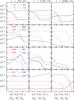 |
Fig. 1 Evolution of the abundances (by mass fraction) of various elements (as indicated in the leftmost panels) as a function of the consumed hydrogen fraction (used as a proxy for time), for three different values of constant temperature (as indicated at the top of the figure) and for a constant density of ρ = 10g cm3. |
The results of our calculations for three different values of the temperature appear in Fig. 1. The abundances of selected C, N, O, Ne, Na, Mg, Al, Si, Ar, and K isotopes are plotted as a function of consumed mass fraction of hydrogen ΔX/X0 = (X0–X)/X0.
The top row shows that the CN isotopes rapidly reach their equilibrium values, on a timescale shorter than the leftmost value on the time axis of the figure4, while O reaches equilibrium when ~1% of H is burned. All these isotopes keep their equilibrium values up to H exhaustion for the whole range of temperatures explored here. The carbon isotopic ratio in particular decreases from the assumed initial value of 210 to low values between 3.7 and 30 respectively for burning temperatures of 75 and 200 MK.
23Na (second row) is produced through the destruction of 22Ne already at 25 MK (not shown here). As temperature increases, an increasing fraction of 20Ne is converted to 22Ne and 23Na. The equilibrium value of 23Na is highest around T = 50 MK and decreases slowly at higher T; at 100 MK the equilibrium value is smaller than the initial value, i.e. 23Na is destroyed.
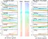 |
Fig. 2 Left: evolution of the abundances (by mass fraction) of various elements as a function of increase in He mass fraction ΔY (used as a proxy for time), for different values of constant temperature (as indicated by the colour-coded values in the middle column), and for a constant density of ρ = 10g cm3; abundances are now expressed as [X/X0] = log(X) – log(X0), where X0 is the initial value. The horizontal bars in each panel indicate the differences between the extreme abundances (Δ[X/Fe] = [X/Fe]E – [X/Fe]0) observed in NGC 2808 (see Table 1). Their thick portion extends between ΔY = 0.02 and 0.04, the variation observed in most globular clusters, while the thin portion extends up to ΔY = 0.15, derived for NGC 2808 (see text for references). Right: same as on the left, but this time the equilibrium abundances of oxygen (which displays the largest depletion with respect to its initial value) are diluted by a factor f with pristine material to fix the observed extreme value in NGC 2808 for each temperature. That factor f, appearing in the middle column for each temperature, is then used to dilute all other abundances. Points are used for temperatures of 75 and 80 MK, where the curves for Na, Mg and Al match the observations (horizontal bars). |
24Mg (third row) is affected only above 70 MK, and only 1% of its initial abundance is left at T = 80 MK. Early on (small H fractions consumed), its destruction leads to an increase in the abundances of 25Mg and 26Al. When more H is consumed, almost all initial Mg (all three isotopes) has turned into 27Al. At temperatures higher than 100 MK, 27Al is destroyed quite rapidly, the amount of consumed H decreasing with increasing temperature. 27Al undergoes an important overproduction in a limited range of temperatures, around 75–90 MK, as already discussed in PCI07.
The bottom panel of Fig. 1 displays the evolution of Si, Ar, and K. Above 100 MK, Si is overproduced from the increased leakage out of the Mg-Al cycle that starts at ~65 MK (e.g. Arnould et al. 1999). Above 180 MK, Si starts being destroyed. The abundances of the heavier isotopes (Ar and K) are not affected by nuclear reactions until temperatures reach above 150 MK when 36Ar is depleted to the profit of 38Ar. Production of 39K occurs only above 170 MK when almost all the 36Ar has gone. 39K reaches a maximum overabundance at 200 MK when it shares with 38Ar almost all the initial abundance of 36Ar. It displays then an overabundance of a factor of 30 with respect to its initial value. This is practically the maximum abundance that K can reach in our set-up (i.e. with the assumed initial abundances), because at even higher temperatures it is destroyed by (p, γ) reactions.
When K gets to such high abundances, all major lighter species – i.e. those participating in the NeNa and MgAl cycle as well as Si – have essentially disappeared. Moreover, more than 30% of the initial H has been consumed in that case; this has some important consequences, as will be discussed in the next section. Finally, it should be noted that Ar and K never reach equilibrium values, in contrast to the cases of the isotopes of CNO or Ne-Na cycles.
4. Comparison to NGC 2808
In this section, we use the nucleosynthesis calculations presented in Sect. 3 to infer the temperatures in the H-burning zones of the “polluters” that affected the composition of the intracluster gas out of which NGC 2808 2P stars formed. In Sect. 4.1, we use the extreme abundances of Table 1 to infer the range of appropriate temperatures, and we summarize the key nucleosynthesis points in Sect. 4.3. We explore the whole abundance pattern of NGC 2808 in Sect. 4.4.
4.1. From extreme to predicted abundances after dilution
In Fig. 2 we show the elemental overabundances of O, Na, Mg, Al, Si, and K (from top to bottom) as function of ΔY, the increase in the He mass fraction, for all the temperature values of our calculations. Results are plotted in the left panel as over- or underabundances [X/X0] with respect to the initial values of those elements, i.e. those corresponding to NGC 2808 1P stars. In the logarithmic scale adopted in the figure, the value of 0 for [X/X0] represents the initial value of the element.
The results can be understood in terms of the isotopic abundance evolution already analysed after Fig. 1, taking into account for example that the abundance of Mg in Fig. 2 (left) is the sum of 24Mg+25Mg+26Mg+26Al in Fig. 1. We also indicate with a horizontal bar in Fig. 2 the maximum variation (i.e. the positive or negative difference), from [X/X0 ] in the abundance of each of the plotted elements, as observed in NGC 2808 and given in Table 1. The bar extends from the lowest values ΔY = 0.02 to 0.04 derived by multiwavelength photometry in other GCs and up to ΔY = 0.15, which is the mean enrichment value evaluated for NGC 2808 (see references in Sect. 2). In the case of oxygen, the extreme observed variation is −1.3 dex, i.e. O is depleted by a factor of 20 in the most extreme 2P stars of NGC 2808.
For the whole temperature range covered by the computations, the O equilibrium values in the left top panel of Fig. 2 are reached at the very beginning of H-burning (i.e., for ΔY much lower than the maximum value allowed by the observations not only for NGC 2808 but also for the other GCs; moreover, the higher the temperature, the lower the value of ΔY at which O reaches equilibrium). Additionally, they lie systematically below the observed extreme abundance of that element in NGC 2808. This suggests that this extreme abundance (and, by extension, the less extreme ones) were obtained by diluting one part of processed material from the H-burning region with f parts of pristine one. As shown in PCI07 for the case of NGC 6752, the whole abundance pattern of GCs can be interpreted in terms of abundances produced by hydrostatic H-burning in a temperature range, diluted with pristine material (having the same composition as the initial one adopted in the calculations) by various factors. Prantzos et al. (2007) adopted a simple formalism for the abundances (mass fractions) of the mixture (=2P stars), namely  (1)where f is the dilution factor, i.e. one part of processed material is mixed with f parts of unprocessed one. The required minimum dilution factors fmin (i.e. those needed to obtain the observed extreme value of O in NGC 2808) for each temperature are then obtained as
  (2)where we take the values for XO,extreme and XO,original from Table 1. The corresponding values of fmin for each temperature appear in the second column of the central part of Fig. 2. They are quite small, in the range from 0.03 to 0.05, implying that the observed extreme values of O in NGC 2808 are obtained from material processed at nuclear burning temperatures, which has been diluted with very little pristine material. The implications of such a small dilution factor are discussed in Sect. 4.2.
These dilution factors fmin are then applied to all the abundances in the left panels and the results appear in the right panels of Fig. 2. All equilibrium values of O correspond now to the extreme values observed in NGC 2808 (by construction). In the case of the other elements, extreme observed values for Na, Mg, and Al are obtained for temperatures in the range 75 to 80 MK (indicated by filled circles in the right panels in Fig. 2), as already shown in PCI07. This happens for maximum variations in He mass fraction in agreement with the observational constraints for ΔY in NGC 2808 (0.15 to 0.2) for the whole temperature range considered here. In addition, the higher the temperature, the lower the variation in He mass fraction at which the predictions match the Mg data. Therefore, in the case of other GCs where ΔY is determined to be significantly lower than in NGC 2808 (i.e., of the order of 0.02 to 0.04), a temperature of ~80 MK is required to fit the observed extreme values of Mg at very low He-enrichment.
In the 75–80 MK temperature range, Si and K variations are negligible. In order to obtain Si and K overabundances comparable to the extreme observed values in NGC 2808, temperatures of >100 MK and 190 MK are required, respectively. However, at such high temperatures, Na, Mg and Al are largely depleted.
4.2. Implications for dilution
In the previous section we show that O rapidly reaches its equilibrium value when ~1% of H is burned and that it is the most affected element; its abundance is reduced by a factor of 50–500 in the studied temperature range. Such low O values are never observed in GCs (although for the most O-poor stars data analysis provides only upper limits for this element), implying that some mixing of burned material with pristine material takes place before the formation of 2P stars. The corresponding dilution factor is determined by the observed extreme O abundance and it is generally quite small, generically less than 10%.
Prantzos et al. (2007) found that in the case of NGC 6752, where the observed lowest O abundance is only ~5 times smaller than the pristine one, the corresponding minimal dilution factor is fmin ~ 30%, i.e. considerably higher than in the case of NGC 2808.
The minimal dilution factor fmin found for NGC 2808 is extremely constraining for all scenarios of 2P star formation. It implies that the extreme 2P stars of NGC 2808 are made from H-processed material essentially unmixed with the gas from which the 1P stars were made. It also has a clear implication concerning the presence of a fragile element, like Li. In the case of NGC 6752, Prantzos et al. (2007) showed that the Li abundance of the most Na-rich stars of that cluster (a factor of ~3 below the so-called “Spite-plateau”; e.g., Spite & Spite 1982; Charbonnel & Primas 2005; Meléndez et al. 2010) can be explained by assuming a mixture of H-processed Li-free material with Li-normal pristine gas with the derived dilution factor of 30%. The dilution factors we derived in PCI07 and in the present study agree with those derived for the mixture between the stellar winds and the original matter in the case of the FRMS scenario based on Li observations (e.g. Decressin et al. 2007b; note that although this approach differs from that of Salaris & Cassisi 2014; who study dilution of Li-free polluters ejecta directly within pre-main sequence stars in the early-disc accretion scenario of Bastian et al. 2013, these authors also conclude for the need to mix polluters yields with gas containing pristine Li). Now, our smaller dilution factor of ~5% for NGC 2808 implies that the initial Li content of the most extreme 2P stars of that cluster has to be even lower, about a factor of 10 below the Spite plateau. We are not aware of Li observations in NGC 2808 as function of e.g. O/Fe or Na/Fe, but we urge such observations, as we find them crucial for the validity of all scenarios proposing 2P star formation from mixing of processed and pristine material in GCs. Such observations should however focus on main sequence stars only, as Li is quickly depleted in subgiant and red giant stars under the effects of the first dredge-up and other mixing processes. Even in the case of main sequence stars actually, the interpretation of the Li observations in GCs requires great caution, as its surface abundance may vary under the action of atomic diffusion combined to rotation-induced turbulent processes (for a review and references, see Charbonnel 2016).
Finally, the carbon isotopic ratio obtained after dilution with a minimum dilution factor of 0.0455 (as found for H-burning temperature of 75–80 MK, see Fig. 2) is 12C/13C = 4.4. This is in agreement with the ratio derived for a handful of subgiant stars in a couple of GCs (NGC 6752 and 47 Tuc; Carretta et al. 2005) but not yet in NGC 2808. As discussed by Charbonnel et al. (2014), the determination of this quantity in turnoff GC stars could provide a new signature of membership to the first and second stellar populations.
4.3. Inferences on H-burning temperature
Applying the above-mentioned mixing/dilution factor fmin to all the other elements (i.e. those less affected than O), we find the following:
-
observed extreme values for Na, Mg, and Al inNGC 2808 can be obtained formaterial that has been processed in thetemperature range 75–80 MK, in agreement withPCI07 finding for NGC 6752;
-
the corresponding predicted He enrichment agrees with the observational constraints on ΔY for NGC 2808. Lower values of ΔY like those observed in other GCs require temperature of the order of 80 MK to fill the Mg constrain;
-
for extreme overabundances of Si and K, temperatures higher than 100 and 190 MK, respectively are required, but then Na, Mg and Al are destroyed. This implies that high K abundances are not expected to be seen in Na- and Al-enriched stars in the case of a single nucleosynthesis source for GC abundance anomalies.
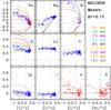 |
Fig. 3 Theoretical abundances of various elements of Fig. 2 obtained at ΔY = 0.15 are diluted by various amounts of pristine material and plotted as function of the corresponding values of [O/Fe] for selected values of temperature (colour-coded lines). Data for NGC 2808 are from Carretta (2014, 2015, blue) and Mucciarelli et al. (2015, red). Typical error bars are of the order of 0.1 dex as quoted in the original papers. |
4.4. Abundance pattern of NGC 2808
In the previous section, we determined the factor fmin required to explain the extreme abundances of NGC 2808 for O and found it to be very small, less than 10%.
We use this simple scheme here, assuming that Xprocessed for each temperature is the value obtained in the simulations when ΔY = 0.15 (see Fig. 2). This choice automatically ensures that i) O will be at its equilibrium value, so we can start dilution with the fmin values of the previous paragraph and ii) the corresponding He abundance will be the extreme value observed in NGC 2808.
In Fig. 3 we display the results of Na, Mg, Al, Si, Ca, Ti, Sc, Cr, and K as functions of O, as well as K vs. Na, for various temperatures and for increasing higher values of the dilution factor f, starting with fmin. We compare our predictions with NGC 2808 observations (Carretta 2014, 2015; Mucciarelli et al. 2015). Since our step in temperature is 5 MK, we can only perform a coarse-grained analysis of the situation; a smaller step would be required for a finer analysis.
The patterns for Na and Al are correctly reproduced for T = 75 MK, but Mg fits better at T = 70 MK and disappears above that temperature when ΔY = 0.15. The Si pattern fits best at T = 80 MK. Taking into account observational error bars, of the order of 0.1 dex in most cases we find that the temperature range of 70–80 MK is the one that best reproduces the patterns. This is similar to our conclusion in PCI07, which concerned NGC 6752, while here we also include Si and the ΔY constraint.
We find that the K vs. O pattern can be obtained for T ≥ 180 MK in these conditions. However, at this temperature Na and most other elements have already been depleted to very low values and the K-Na correlation observed in NGC 2808 is not predicted at any temperature. This inconsistency is obtained whatever the He abundance variations, i.e. independently of the He constraint. Similarly, the computations predict a K-Al anticorrelation, at odds with the data.
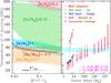 |
Fig. 4 Left: shaded areas indicate the temperature range as a function of produced He amount (ΔY) where each of the corresponding elements is either overproduced (Na, Al, Si and K) or depleted (Mg) with respect to its initial value by the factors indicated; these factors correspond to the extreme abundances observed in NGC 2808 (see Table 1). The horizontal bar at the bottom corresponds to the observationally inferred variation in the He content of most globular clusters (thick portion) and of NGC 2808 (thin portion; see Sect. 2). The boxes around the Mg values correspond to these inferred variations and show explicitly why Mg is the most sensitive “thermometer” among those elements (see text). Right: H-burning temperatures at various phases of a star’s life as a function of initial stellar mass (see legend at the top of the figure, adapted from Prantzos et al. 2007). Vertical red segments (for central H-burning) start at the ZAMS and end at central H mass fraction X = 0.01 (thick portion) and X = 0 (thin portion, for stars between 20 and 200 M⊙). For the other phases we show only the maximum temperature reached in the H-burning zones of interest. In the bottom part, more details are given for massive star evolution. On the right side of the figure the temperatures are for the supermassive star models of Denissenkov (priv. comm.). The shaded rectangular area indicates the “triple point”, i.e. the temperature range (from the left side) allowing for the co-production of Na, Mg, and Al at the levels inferred from observations of NGC 2808. |
5. Implications for the polluter candidates
5.1. T vs. ΔY constraints for hydrostatic H-burning
In Sect. 4.1 we determined the temperature conditions that allow the production/destruction of the key elements O, Na, Al, Mg, Si, and K to their extreme abundance levels, as observed in NGC 2808 and considering the He constraint. In Sect. 4.4 we showed that within a simple scheme of dilution of these abundances with pristine material, a large amount of the observed patterns in NGC 2808 can be reduced. However, even if some correlations/anticorrelations are satisfactorily reproduced, this does not always occur for the same range of temperatures. Furthermore, some observed correlations (K-Na and K-Al) are never reproduced.
The situation is summarized on the left side of Fig. 4. It displays the temperature ranges where each of the key elements reaches (after dilution) its extreme abundance, as observed in NGC 2808 and indicated by the corresponding numbers. The temperature ranges are displayed as a function of the increased ΔY in He mass fraction. We indicate the observationally inferred variation in He content for NGC 2808 and other GCs. It can be seen that Na and Al “coexist” at their observed highest level in a narrow range around T ~ 75–80 MK at low ΔY (compatible with the relatively high He values derived for NGC 2808 and with the much lower He values obtained in several GCs), which extends down to 60–80 MK at H-exhaustion (ΔY~ 0.75). Na drops below its extreme value above T ~ 80 MK, and Al above 80–90 MK, depending on the amount of He. At low ΔY values, Si is produced after Al decreases from its maximum abundance. For larger ΔY, Si may coexist at its observed level with large Al amounts around 90 MK and even with Na around 80 MK, but only for ΔY values larger than derived observationally in NGC 2808. K is produced for relatively high ΔY (still compatible with ΔY in NGC 2808, but not with ΔY < 0.04). However, and as already noted before, K production occurs only at extremely high temperatures where Na, Al, and Mg are destroyed; it is marginally compatible with Si enhancement for very high ΔY beyond the observational constraint.
An interesting feature is the very narrow temperature range where Mg displays its observed depletion of [Mg/Mg0] ~ −0.5 dex in NGC 2808: a narrow band of width ΔT ~ 5 MK extending from T ~ 80 MK at ΔY = 0.02 to T ~ 70 MK at ΔY = 0.15. In PIC2007 we showed that the isotopic abundances of Mg are co-produced at the levels observed in NGC 6752 for T ~ 75 MK, but for smaller ΔY values. The derived narrow temperature range suggests that the abundance of Mg constitutes the most sensitive thermometer to probe the conditions of the astrophysical site of the polluter(s); the increase in the He abundance constitutes a second parameter in that respect. This is a key finding of our study.
5.2. Hydrostatic H-burning sources
5.2.1. H-burning temperature in stellar models
We now check whether the above-mentioned nucleosynthetic requirements for NGC 2808 correspond to the temperature conditions of hydrostatic H-burning in specific astrophysical sites. We consider single stars in the whole range of masses between 1 and 200 M⊙ (while in PCI07 we only considered stars up to 120 M⊙), as well as the putative supermassive stars above 103M⊙ that have been proposed as polluters of GCS (Denissenkov & Hartwick 2014). We also consider H-burning shells of red giants and AGB stars.
The results are summarized in the right panel of Fig. 4 where we plot, on the same scale as on the left, the temperatures of the various putative polluters as function of the initial stellar mass. We collect predictions from stellar model computed by various authors at [Fe/H] = −1.5. The models with masses between 20 and 120 M⊙ are from Decressin et al. (2007b), and the 200 M⊙ model was computed with the same version of the Geneva stellar evolution code for the present study (C. Georgy, priv. comm.). The models with masses lower than 9 M⊙ are a combination from Decressin et al. (2009), Pumo et al. (2007), and Ventura et al. (2002). Finally, the models for supermassive stars have been computed by P. Denissenkov (priv. comm.) with the stellar evolution code MESA (Paxton et al. 2011, 2013) using the same physical assumptions as in Denissenkov et al. (2015).
The correspondence between symbols and evolutionary phases is displayed in the upper left part of the figure (adapted from PCI07). Vertical red segments (for central H-burning) start at the ZAMS and end at central H-exhaustion. We also indicate with small horizontal tick marks the temperatures where ΔY~ 0.15 (i.e. maximum He enrichment in NGC 2808) and with triangles the temperatures where ΔY~ 0.55 (i.e. 20% of H left). For the other phases we show only the maximum temperature reached in the H-burning zones of interest (i.e. H-burning shell for stars at the RGB tip and at the clump, and the base of the convective envelope for stars undergoing thermal pulses on the AGB).
A comparison of the left and right diagrams of Fig. 4 allows us to draw the following straightforward conclusions for the different potential polluters5. Here we focus on the nucleosynthesis aspects. We refer to recent reviews for an extended discussion about more general issues related to the associated GC pollution scenarios (e.g. Renzini et al. 2015; Bastian 2017; Charbonnel 2016, 2017).
5.2.2. Fast rotating massive main sequence stars
Our computations confirm that central H-burning in massive stars (20 to 200 M⊙) can produce the observed large Na excess and O depletion (i.e. the defining chemical feature of GC stars) for relatively low ΔY values, corresponding to the range observed in GC 2P stars (i.e. between 0.01 and 0.2). In contrast, the observed high Al values and the observed Mg depletion can be obtained for massive main sequence star temperatures only for large increases in the He content (i.e. towards H-exhaustion), substantially larger than inferred from GC observations. A similar conclusion holds for Si: large amounts, i.e. comparable to observed values, can be obtained at T ≥ 80 MK but only for high He abundances; however, at such high temperatures Mg is always destroyed. Finally, no K can be produced in these objects.
Our results agree with the nucleosynthesis predictions of the evolution models of fast rotating massive stars (FRMS, see e.g. Figs. 3 and 6 of Decressin et al. 2007b). In the original FRMS scenario, the hydrogen-burning ashes would be ejected from massive stars rotating near critical rotation velocity all along the main sequence and would mix with pristine gas to form 2P stars in the immediate surroundings of the massive parent star. Since the CNO-cycle and the NeNa chain fully operate at relatively low temperature at the beginning of the main sequence, the FRMS models naturally explain the O-Na anticorrelation for moderate He enrichment as derived for NGC 2808 or even lower (e.g. Chantereau et al. 2015). Additionally, it has been predicted that 2P stars are born with relatively low carbon isotopic ratios (Charbonnel et al. 2014).
However, 2P GC stars with important Al excess and Mg depletion can be made only from high-temperature material of FRMS close to H-exhaustion, having therefore a high He mass fraction (up to Y = 0.8 after dilution with pristine gas; see e.g. Fig. 1 of Chantereau et al. 2016). Here, we confirm this conclusion. In particular, the difficulty in reproducing the Mg-Al anticorrelation was already pointed out by Decressin et al. (2007b), who showed that in the typical case of NGC 6752, this pattern could be reproduced by FRMS models only by invoking an increase in the 24Mg(p, γ) reaction rate by a factor of 1000 around 50MK with respect to the nominal rate of Iliadis et al. (2001). Such a large increase is extremely unlikely, given the quality of current input nuclear physics information for this rate. Even in this case, Mg-depletion would come with strong He enrichment.
Whether or not this can detected in the GC CMDs remains unclear. In the original FRMS scenario, only ~20% of 2P in NGC 2808 are expected to be born with an initial ΔY higher than 0.15 (Chantereau et al. 2016). Because of the effects of He on the stellar evolution paths and lifetimes (Chantereau et al. 2015, and references therein), their total number reduces to ~10% at the main sequence turnoff and on the RGB for GCs with ages between 9 and 13 Gyr. Additionally, for the same age range, this fraction drops dramatically on the horizontal branch (~0.5% at 13 Gyr), meaning that this evolution phase cannot be used to distinguish between the two most commonly invoked scenarios for GC enrichment. These very helium-rich 2P stars might even disappear on the AGB, depending on the age and metallicity of their host GC, and on their mass loss rate along the RGB (Charbonnel et al. 2013; Cassisi et al. 2014; Charbonnel & Chantereau 2016; Chantereau et al. 2016).
5.2.3. Supermassive main sequence stars
The situation appears to be more favourable in the case of supermassive main sequence stars (SMSs) with masses above 2 × 10³M⊙. According to the stellar models we plot in Fig. 4, their central temperatures are already high enough at the beginning of the main sequence to allow for a simultaneous co-existence of He, Na, Al and Mg to levels compatible with observational constraints (except for SMS with mass M > 104M⊙). For these elements, our computations are in good agreement with the model predictions of Denissenkov et al. (2015, see e.g. their Fig. 1 for maximum ΔY. In addition, our computations show that Si can also be produced in that site, but at temperatures where Mg is heavily depleted. When both constraints are considered, i.e. T and ΔY, we find that neither Mg nor Na survives Si production. Finally, we show that the current SMS models do not reach K-production temperature.
As can be seen in Fig. 4, the models predict a strong increase in the central temperature as SMSs evolve along the main sequence, in particular once ΔY reaches 0.55 (central He mass fraction of 0.8), which leads to Na and Al depletion, at odds with the observations. Therefore, if SMSs played a role in GC pollution, they must have released H-burning material at the very beginning of the main sequence, as proposed by Denissenkov & Hartwick (2014) based on the He argument. Whether this can happen requires the verification of speculations on how the required mass loss might be driven by the super-Eddington radiation continuum-driven stellar wind or by the diffusive mode of the Jeans instability.
5.2.4. Asymptotic giant branch stars
For the case of AGB stars, conclusions are not straightforward because the simple one-zone calculations at constant T performed here cannot capture the complexity of the situation. In addition to hot-bottom burning in the AGB envelope, which is invoked for the required hot H-burning, the third dredge-up events can occur and can mix material of He-burning in H-burning zones, altering the composition of the latter and the products of nucleosynthesis (for details, see e.g. Charbonnel 2016). The range of AGB temperatures reported in Fig. 2 thus simply indicates that the abundances of Na, Mg, Al, O, and Si can be modified in that site, while K cannot, but it gives no clues as to the resulting correlations or anticorrelations between these elements, which are strongly determined by the mixing with He-burning material. For example, all the AGB and super-AGB models computed so far predict chemical yields at odds with the observed O-Na anticorrelation (e.g. Forestini & Charbonnel 1997; Denissenkov & Herwig 2003; Karakas & Lattanzio 2007; Siess 2010; Ventura et al. 2013; Doherty et al. 2014), exactly because of the competition between the third dredge up and HBB (for details see e.g. Charbonnel 2016).
Moreover, models of rotating AGB stars predict the ejection of helium-burning products by these stars (Decressin et al. 2009). During central He-burning, rotational mixing does indeed bring fresh CO-rich material from the core towards the hydrogen-burning shell, causing important production of primary 14N that is later mixed in the stellar envelope during the second dredge-up. This strongly increases the total C+N+O content at the stellar surface and in the stellar wind (this adds to the C+N+O increase already predicted by standard, non-rotating models, see e.g. Karakas et al. 2006). While this prediction is sustained by a wide variety of galactic observations (e.g. Maeder & Meynet 2006; Chiappini et al. 2008), in the case of GCs it would imply that 2P stars present higher total C+N+O values than their 1P counterparts. This at odds with the constancy of C+N+O observed among GC low-mass stars which otherwise present strong variations in the individual abundances of C, N, O, and Na (references in Sect. 1).
The temperature range for hot bottom burning by the AGB models shown in Fig. 4 does not reach the values that are necessary to produce K. This is totally consistent with the results of Ventura et al. (2012) when they use the current nuclear reaction rates available for the reactions involved in the production of this element. These authors thus call for an increase in the 38Ar(p, γ39)K cross section by a factor of 100 to produce K in AGB models. However, an increase of this magnitude seems unlikely, considering the nuclear physics input. As an alternative, Ventura et al. (2012) suggest that HBB temperature might be higher in AGB stars than the current models predict. In that case, the computations presented in the present paper show that the corresponding yields would then be devoid of Na, Al, and Mg, as discussed previously.
Finally, our computations do not provide any information on the amount of He that is produced by AGB stars and released in their winds together with the H- and He-burning products. In the case of these potential polluters, He enrichment indeed comes from the second dredge-up that occurs on the early-AGB phase (He enrichment due to HBB is negligible). As a consequence, the He yields on the one hand and those of CNONaMgAl nuclei on the other are not directly correlated since these elements are processed at different phases of the evolution. In all the AGB models available (references above), the He content of the ejecta increases with polluter mass, and Y reaches a value of ~0.38 for the most massive AGBs. All 2P stars are thus expected to share similar and relatively high initial He abundances, independently of their CNONaMgAl content.
5.3. The peculiar case of K: a hint of novae?
Among the various abundance patterns reported so far for GC stars, the overabundance of potassium in the most massive GCs like NGC 2808, if real, is undoubtedly the most disturbing. None of the known or putative stellar sources discussed in the previous section is expected to reach the H-burning temperatures as high as >180 MK that are required to produce K in excess.
H-burning at such high – or even higher – temperatures is expected to occur in novae, but explosively, i.e. on a hydrodynamical timescale τ = ρ− 1/2 (where ρ is the peak density of the exploding region), which is always shorter than the nuclear timescale; as a result, only a small fraction of the main nuclear fuel is consumed. Still, important modifications to the abundances of other nuclear species may occur.
Detailed theoretical investigations have shown that the nova outburst is a multi-parameter phenomenon, depending on the mass, temperature and composition of the exploding white dwarf, and on the accretion rate and composition of the material of the companion star, etc. (see e.g. José 2017, for a recent review). In these conditions, it is not easy to perform parametrized simulations of nova nucleosynthesis. Still, detailed 1D simulations clearly suggest that peak temperatures much higher than 200 MK, sometimes reaching 450 MK can be obtained (e.g. Yaron et al. 2005; Denissenkov et al. 2014).
In particular, Denissenkov et al. (2014) studied models of CO and ONe white dwarfs with the MESA code, performing post-processing nucleosynthesis with the NUGRID multi-zone code MPPNP. They used a network of 147 species, up to Ca-47 and thus appropriate for K production; 1700 nuclear reactions are considered, with rates taken for JINA Reaclib v1, which include those evaluated by Iliadis et al. (2010).
An inspection of the results presented in Denissenkov et al. (2014) shows that a modest overabundance of K can be obtained in some cases. However, in all these cases, all intermediate mass elements (Na, Al, Si, S) are systematically overproduced to large amounts, much larger than observed; sometimes O is also overproduced, in contrast with its well-known depletion in GCs. The reason is that such elements are made from abundant “seed” material (CO or ONe white dwarfs) and explosive nucleosynthesis has little time to substantially deplete the original elements. Based on these results, it is tempting to conclude that K overproduction in novae is expected to be accompanied by much larger overproduction of lighter elements. This conclusion would be in stark contrast with the one on hydrostatic H-burning presented in Sect. 4.2. However, a much more thorough investigation of the large parameter space of novae would be required to establish this conclusion on a firm basis.
The issue of novae as potential sources of K anomalies in the 2P stars of GCs is also discussed in Iliadis et al. (2016) from the point of view of the total mass available for star formation in that case. They find that for the case of NGC 2419, novae could eject enriched material to form at most 1% of the K-enriched stars observed in that cluster (which constitute about 30% of the total population). However, they point out that current models of novae, concerning white dwarfs accreting from their companion stars, are perhaps not appropriate to account for the situation in the early life of GCs, where accretion would take place directly from the fairly dense (~106 cm-3) ISM; the total amount of material processed by the white dwarfs of the GC could be much larger in that case. However, the corresponding hydrodynamical problems concerning the retention of the fast ejecta within the cluster in order to form the 2P stars, have not yet been considered.
6. Summary
In this work, we reassess the nucleosynthesis constraints on the putative polluters of 2P stars in GCs. We consider the specific case of NGC 2808, where abundances for elements up to K have been reported to display variations among the cluster stars. We study H-burning nucleosynthesis in hydrostatic conditions, as appropriate for almost all polluter sites proposed so far. We perform parametrized calculations, varying the temperature in the range of 20 to 200 MK and keeping the density constant at 10 g cm3.
In the spirit of our previous study (Prantzos et al. 2007, where we focused on NGC 6752) we first determined the conditions reproducing the most extreme abundances reported in one specific GC, namely NGC 2808. We find that it is possible to reproduce the extreme abundances of O, Na, Al and Mg for T ~ 75–80 MK, after a small dilution with pristine material (i.e. having the composition of the 1P stars in the cluster). The small dilution factor, of the order of ~5%, was determined by the abundance of oxygen, which is the most affected heavy element in H-burning. This minimal dilution factor is substantially smaller than determined in PCI07 for NGC 6752 (~30%). This finding is extremely constraining for all scenarios of 2P star formation in GCs, which must account for stochasticity in the formation process of MSPs (Bastian et al. 2015). Here it implies that the extreme 2P stars of NGC 2808 are made from H-processed material essentially unmixed with the gas from which the 1P stars were made. A direct consequence is that the initial Li content of the most extreme 2P stars of that cluster has to be about a factor of 10 below the Spite plateau. We urge then Li observations in NGC 2808 main sequence stars, as we find them crucial for the validity of all scenarios proposing 2P star formation from mixing of processed and pristine material in GCs.
The narrow temperature range between 70–80 MK where the observed extreme values of O, Na, Mg and Al in NGC 2808 can be reproduced (after minimal dilution) is the same as that determined in PCI07 for NGC 6752. Here we show that the abundance of Mg constitutes the most sensitive thermometer, allowing one to probe the conditions of the astrophysical site of the polluter(s). The increase in the He abundance constitutes a second parameter in that respect, allowing for the same abundance of Mg to be obtained either at T ~ 80 MK and low ΔY (~3%) or at lower T ~ 70 MK and higher ΔY (around 10–15%). Finally, we find that the observed extreme Si abundance in NGC 2808 can also be obtained for the high T values of that temperature range, around T ~ 80 MK, and for high values of ΔY~ 0.15.
Ideally, our scheme should allow us to pinpoint more precisely the allowed region in the T vs. ΔY phase space. However, the uncertainties in the observed abundances (~0.1 dex) and in the He content of GC stars, at present preclude that possibility. Moreover, the simplicity of the method – one-zone H-burning, not allowing for replenishment of depleted species through convection – makes it difficult to accurately simulate realistic sites, such as convective core burning in massive stars or hot bottom burning in AGBs. Even so, the resulting abundances are more sensitive to the variations of temperature, thus our results should be considered as reliable first-order approximations of more complex situations.
Once the extreme values of the various elements are obtained (after determining T and fmin), dilution with various factors higher then fmin allows the full abundance pattern of a given GC to be obtained, as shown in PCI07. Here we repeat this exercise for NGC 2808, showing how most of the observed abundance patterns can be satisfactorily obtained from material processed through H-burning at T ~ 70–80 MK. K is a clear exception, since its observed extreme abundance requires T ~ 180 MK at least. At such high temperatures, most of the other key elements (Na, Mg, Al) are heavily depleted and the corresponding patterns do not match the observed ones.
Finally, we discuss the main putative polluters of GCs, namely AGBs, FRMS, and SMS, considering only the nucleosynthesis aspects and not other features of the corresponding scenarios (e.g. the mass budget problem, the retention of the polluter ejecta or their mixing with pristine material, the dependence on the mass, compactness, and metallicity of the cluster). As already emphasized in the literature, AGBs produce correlations rather than the observed anticorrelations between O, Na and Al. Fast rotating massive stars easily make the O-Na extreme abundances but barely reach the temperature regime for the extreme Mg-Al abundances observed in NGC 2808 and in other very massive or metal-poor GC. The latter temperature regime is reached by the hypothetical SMSs resulting in severe depletion of Mg early on the main sequence, i.e. for low ΔY. None of the above-mentioned sources reaches the high T regime required for K production. The only known H-burning site able to do so is novae, but recent models show that abundance patterns substantially different than the observed ones should be expected in that case. To date, K abundance variations have been reported in only two of the most massive galactic GCs. If confirmed, these observations could eventually indicate that specific conditions were ruling the early evolution of such clusters. However, the fact that K and Na are observed to be correlated can not be explained with our current understanding of H-burning nucleosynthesis. Before turning to exotic solutions, we urge observers to investigate possible issues in abundance analysis.
Our conclusion is that, despite two decades of intense theoretical and observational investigation, the origin of the observed abundance anomalies in GCs remains a fundamentally unsettled issue. However, we think that this work convincingly shows that respecting the nucleosynthetic constraints must be the fundamental consideration for all the scenarios that aim to explain the formation of multiple stellar populations in GCs. Although we focus here on the specific case of NGC 2808, one of the most massive GCs that show the most extreme abundance anomalies, our computations can be directly used to constrain the polluter stars that may have played a role in shaping differently (or stochastically) the abundance patterns in other GCs.
The compactness index is usually defined as (M∗/105)/(rh/pc), with M∗ the stellar mass and rh the half-mass radius of a GC. Additionally, Pancino et al. (2017) find that the extent of the Mg-Al anticorrelation also depends on GC [Fe/H] content.
We do not discuss the case of intermediate-mass binary stars (de Mink et al. 2009) since the temperatures in these 10–20 M⊙ objects can only account for Na enrichment, but not for Al enhancement or Mg depletion.
Acknowledgments
We warmly thank P. Denissenkov and C. Georgy for providing stellar models results, and N. Bastian, W. Chantereau, M. Gieles, M. Krause, and C. Lardo for careful reading and useful comments on the manuscript. C.C. acknowledges support from the Swiss National Science Foundation (SNF) for the Projects 200020-159543 “Multiple stellar populations in massive star clusters – Formation, evolution, dynamics, impact on galactic evolution” and 200020-169125 “Globular cluster archeology”. We thank the International Space Science Institute (ISSI, Bern, CH) for welcoming the activities of the Team 271 “Massive Star Clusters Across the Hubble Time” (2013–2016; team leader C.C.).
References
- Arnould, M., Goriely, S., & Jorissen, A. 1999, A&A, 347, 572 [NASA ADS] [Google Scholar]
- Bastian, N. 2016, in EAS Pub. Ser. 80, eds. E. Moraux, Y. Lebreton, & C. Charbonnel, 5 [Google Scholar]
- Bastian, N. 2017, in Formation, Evolution, and Survival of Massive Star Clusters, eds. C. Charbonnel, & A. Nota, IAU Symp., 316, 302 [Google Scholar]
- Bastian, N., Lamers, H. J. G. L. M., de Mink, S. E., et al. 2013, MNRAS, 436, 2398 [NASA ADS] [CrossRef] [MathSciNet] [Google Scholar]
- Bastian, N., Cabrera-Ziri, I., & Salaris, M. 2015, MNRAS, 449, 3333 [NASA ADS] [CrossRef] [Google Scholar]
- Bellini, A., Milone, A. P., Anderson, J., et al. 2017, ApJ, 844, 164 [NASA ADS] [CrossRef] [Google Scholar]
- Bragaglia, A., Carretta, E., Gratton, R., et al. 2010, A&A, 519, A60 [NASA ADS] [CrossRef] [EDP Sciences] [Google Scholar]
- Bragaglia, A., Gratton, R. G., Carretta, E., et al. 2012, A&A, 548, A122 [NASA ADS] [CrossRef] [EDP Sciences] [Google Scholar]
- Bragaglia, A., Sneden, C., Carretta, E., et al. 2014, ApJ, 796, 68 [NASA ADS] [CrossRef] [Google Scholar]
- Busso, G., Cassisi, S., Piotto, G., et al. 2007, A&A, 474, 105 [NASA ADS] [CrossRef] [EDP Sciences] [Google Scholar]
- Caloi, V., & D’Antona, F. 2007, A&A, 463, 949 [NASA ADS] [CrossRef] [EDP Sciences] [Google Scholar]
- Carretta, E. 2006, AJ, 131, 1766 [NASA ADS] [CrossRef] [Google Scholar]
- Carretta, E. 2013, A&A, 557, A128 [NASA ADS] [CrossRef] [EDP Sciences] [Google Scholar]
- Carretta, E. 2014, ApJ, 795, L28 [NASA ADS] [CrossRef] [Google Scholar]
- Carretta, E. 2015, ApJ, 810, 148 [NASA ADS] [CrossRef] [Google Scholar]
- Carretta, E., Gratton, R. G., Bragaglia, A., Bonifacio, P., & Pasquini, L. 2004, A&A, 416, 925 [NASA ADS] [CrossRef] [EDP Sciences] [Google Scholar]
- Carretta, E., Gratton, R. G., Lucatello, S., Bragaglia, A., & Bonifacio, P. 2005, A&A, 433, 597 [NASA ADS] [CrossRef] [EDP Sciences] [Google Scholar]
- Carretta, E., Bragaglia, A., Gratton, R. G., et al. 2009, A&A, 505, 117 [NASA ADS] [CrossRef] [EDP Sciences] [Google Scholar]
- Carretta, E., Bragaglia, A., Gratton, R. G., et al. 2010, A&A, 516, A55 [NASA ADS] [CrossRef] [EDP Sciences] [Google Scholar]
- Carretta, E., Gratton, R. G., Bragaglia, A., et al. 2013, ApJ, 769, 40 [NASA ADS] [CrossRef] [Google Scholar]
- Cassisi, S., Salaris, M., Pietrinferni, A., Vink, J. S., & Monelli, M. 2014, A&A, 571, A81 [NASA ADS] [CrossRef] [EDP Sciences] [Google Scholar]
- Černiauskas, A., Kučinskas, A., Klevas, J., et al. 2017, A&A, 604, A35 [NASA ADS] [CrossRef] [EDP Sciences] [Google Scholar]
- Chantereau, W., Charbonnel, C., & Decressin, T. 2015, A&A, 578, A117 [NASA ADS] [CrossRef] [EDP Sciences] [Google Scholar]
- Chantereau, W., Charbonnel, C., & Meynet, G. 2016, A&A, 592, A111 [NASA ADS] [CrossRef] [EDP Sciences] [Google Scholar]
- Charbonnel, C. 2016, in EAS Pub. Ser. 80, eds. E. Moraux, Y. Lebreton, & C. Charbonnel, 177 [Google Scholar]
- Charbonnel, C. 2017, in Formation, Evolution, and Survival of Massive Star Clusters, eds. C. Charbonnel, & A. Nota, IAU Symp., 316, 1 [Google Scholar]
- Charbonnel, C., & Chantereau, W. 2016, A&A, 586, A21 [NASA ADS] [CrossRef] [EDP Sciences] [Google Scholar]
- Charbonnel, C., & Primas, F. 2005, A&A, 442, 961 [NASA ADS] [CrossRef] [EDP Sciences] [Google Scholar]
- Charbonnel, C., Chantereau, W., Decressin, T., Meynet, G., & Schaerer, D. 2013, A&A, 557, L17 [NASA ADS] [CrossRef] [EDP Sciences] [Google Scholar]
- Charbonnel, C., Chantereau, W., Krause, M., Primas, F., & Wang, Y. 2014, A&A, 569, L6 [NASA ADS] [CrossRef] [EDP Sciences] [Google Scholar]
- Chiappini, C., Ekström, S., Meynet, G., et al. 2008, A&A, 479, L9 [NASA ADS] [CrossRef] [EDP Sciences] [Google Scholar]
- Cohen, J. G. 2004, AJ, 127, 1545 [NASA ADS] [CrossRef] [Google Scholar]
- Cohen, J. G., & Kirby, E. N. 2012, ApJ, 760, 86 [NASA ADS] [CrossRef] [Google Scholar]
- Cohen, J. G., & Meléndez, J. 2005, AJ, 129, 303 [NASA ADS] [CrossRef] [Google Scholar]
- Cohen, J. G., Huang, W., & Kirby, E. N. 2011, ApJ, 740, 60 [NASA ADS] [CrossRef] [Google Scholar]
- Dalessandro, E., Salaris, M., Ferraro, F. R., et al. 2011, MNRAS, 410, 694 [NASA ADS] [CrossRef] [Google Scholar]
- D’Antona, F., & Caloi, V. 2004, ApJ, 611, 871 [NASA ADS] [CrossRef] [Google Scholar]
- D’Antona, F., Bellazzini, M., Caloi, V., et al. 2005, ApJ, 631, 868 [NASA ADS] [CrossRef] [Google Scholar]
- D’Antona, F., Vesperini, E., D’Ercole, A., et al. 2016, MNRAS, 458, 2122 [NASA ADS] [CrossRef] [Google Scholar]
- de Mink, S. E., Pols, O. R., Langer, N., & Izzard, R. G. 2009, A&A, 507, L1 [NASA ADS] [CrossRef] [EDP Sciences] [Google Scholar]
- de Silva, G. M., Gibson, B. K., Lattanzio, J., & Asplund, M. 2009, A&A, 500, L25 [NASA ADS] [CrossRef] [EDP Sciences] [MathSciNet] [Google Scholar]
- Decressin, T., Charbonnel, C., & Meynet, G. 2007a, A&A, 475, 859 [NASA ADS] [CrossRef] [EDP Sciences] [Google Scholar]
- Decressin, T., Meynet, G., Charbonnel, C., Prantzos, N., & Ekström, S. 2007b, A&A, 464, 1029 [NASA ADS] [CrossRef] [EDP Sciences] [Google Scholar]
- Decressin, T., Charbonnel, C., Siess, L., et al. 2009, A&A, 505, 727 [NASA ADS] [CrossRef] [EDP Sciences] [Google Scholar]
- Denisenkov, P. A., & Denisenkova, S. N. 1990, Sov. Astron. Lett., 16, 275 [NASA ADS] [Google Scholar]
- Denissenkov, P. A., & Herwig, F. 2003, ApJ, 590, L99 [NASA ADS] [CrossRef] [Google Scholar]
- Denissenkov, P. A., & Hartwick, F. D. A. 2014, MNRAS, 437, L21 [NASA ADS] [CrossRef] [Google Scholar]
- Denissenkov, P. A., Da Costa, G. S., Norris, J. E., & Weiss, A. 1998, A&A, 333, 926 [NASA ADS] [Google Scholar]
- Denissenkov, P. A., Truran, J. W., Pignatari, M., et al. 2014, MNRAS, 442, 2058 [NASA ADS] [CrossRef] [Google Scholar]
- Denissenkov, P. A., VandenBerg, D. A., Hartwick, F. D. A., et al. 2015, MNRAS, 448, 3314 [NASA ADS] [CrossRef] [Google Scholar]
- D’Ercole, A., D’Antona, F., Carini, R., Vesperini, E., & Ventura, P. 2012, MNRAS, 423, 1521 [NASA ADS] [CrossRef] [Google Scholar]
- di Criscienzo, M., D’Antona, F., Milone, A. P., et al. 2011, MNRAS, 414, 3381 [NASA ADS] [CrossRef] [Google Scholar]
- di Criscienzo, M., Tailo, M., Milone, A. P., et al. 2015, MNRAS, 446, 1469 [NASA ADS] [CrossRef] [Google Scholar]
- Dickens, R. J., Croke, B. F. W., Cannon, R. D., & Bell, R. A. 1991, Nature, 351, 212 [NASA ADS] [CrossRef] [Google Scholar]
- Doherty, C. L., Gil-Pons, P., Lau, H. H. B., Lattanzio, J. C., & Siess, L. 2014, MNRAS, 437, 195 [NASA ADS] [CrossRef] [Google Scholar]
- D’Orazi, V., Lucatello, S., Gratton, R., et al. 2010, ApJ, 713, L1 [NASA ADS] [CrossRef] [Google Scholar]
- Dupree, A. K., & Avrett, E. H. 2013, ApJ, 773, L28 [NASA ADS] [CrossRef] [Google Scholar]
- Forestini, M., & Charbonnel, C. 1997, A&AS, 123, 241 [NASA ADS] [CrossRef] [EDP Sciences] [Google Scholar]
- Geisler, D., Villanova, S., Carraro, G., et al. 2012, ApJ, 756, L40 [NASA ADS] [CrossRef] [Google Scholar]
- Goswami, A., & Prantzos, N. 2000, A&A, 359, 191 [NASA ADS] [Google Scholar]
- Gratton, R. G., Carretta, E., Bragaglia, A., Lucatello, S., & D’Orazi, V. 2010, A&A, 517, A81 [NASA ADS] [CrossRef] [EDP Sciences] [Google Scholar]
- Gratton, R. G., Carretta, E., & Bragaglia, A. 2012, A&ARv, 20, 50 [CrossRef] [Google Scholar]
- Harris, W. E. 2010, ArXiv e-prints [arXiv:1012.3224] [Google Scholar]
- Hollyhead, K., Kacharov, N., Lardo, C., et al. 2017, MNRAS, 465, L39 [NASA ADS] [CrossRef] [Google Scholar]
- Iben, I. 1968, Nature, 220, 143 [NASA ADS] [CrossRef] [Google Scholar]
- Iliadis, C., D’Auria, J. M., Starrfield, S., Thompson, W. J., & Wiescher, M. 2001, ApJS, 134, 151 [NASA ADS] [CrossRef] [Google Scholar]
- Iliadis, C., Longland, R., Champagne, A. E., Coc, A., & Fitzgerald, R. 2010, Nucl. Phys. A, 841, 31 [NASA ADS] [CrossRef] [Google Scholar]
- Iliadis, C., Karakas, A. I., Prantzos, N., Lattanzio, J. C., & Doherty, C. L. 2016, ApJ, 818, 98 [NASA ADS] [CrossRef] [Google Scholar]
- Ivans, I. I., Sneden, C., Kraft, R. P., et al. 1999, AJ, 118, 1273 [NASA ADS] [CrossRef] [Google Scholar]
- José, J. 2017, in 14th International Symposium on Nuclei in the Cosmos (NIC2016), eds. S. Kubono, T. Kajino, S. Nishimura, et al., 010501 [Google Scholar]
- Karakas, A. I. 2010, MNRAS, 403, 1413 [NASA ADS] [CrossRef] [Google Scholar]
- Karakas, A., & Lattanzio, J. C. 2007, PASA, 24, 103 [NASA ADS] [CrossRef] [Google Scholar]
- Karakas, A. I., Fenner, Y., Sills, A., Campbell, S. W., & Lattanzio, J. C. 2006, ApJ, 652, 1240 [NASA ADS] [CrossRef] [Google Scholar]
- Kimmig, B., Seth, A., Ivans, I. I., et al. 2015, AJ, 149, 53 [NASA ADS] [CrossRef] [Google Scholar]
- King, I. R., Bedin, L. R., Cassisi, S., et al. 2012, AJ, 144, 5 [NASA ADS] [CrossRef] [Google Scholar]
- Krause, M., Charbonnel, C., Decressin, T., Meynet, G., & Prantzos, N. 2013, A&A, 552, A121 [NASA ADS] [CrossRef] [EDP Sciences] [Google Scholar]
- Krause, M. G. H., Charbonnel, C., Bastian, N., & Diehl, R. 2016, A&A, 587, A53 [NASA ADS] [CrossRef] [EDP Sciences] [Google Scholar]
- Kubryk, M., Prantzos, N., & Athanassoula, E. 2015, A&A, 580, A126 [NASA ADS] [CrossRef] [EDP Sciences] [Google Scholar]
- Kudryashov, A. D., & Tutukov, A. V. 1988, Astronomicheskij Tsirkulyar, 1525, 11 [NASA ADS] [Google Scholar]
- Langer, G. E., Hoffman, R., & Sneden, C. 1993, PASP, 105, 301 [NASA ADS] [CrossRef] [Google Scholar]
- Lee, Y.-W., Joo, S.-J., Han, S.-I., et al. 2005, ApJ, 621, L57 [NASA ADS] [CrossRef] [Google Scholar]
- Lee, Y.-W., Han, S.-I., Joo, S.-J., et al. 2013, ApJ, 778, L13 [NASA ADS] [CrossRef] [Google Scholar]
- Lind, K., Primas, F., Charbonnel, C., Grundahl, F., & Asplund, M. 2009, A&A, 503, 545 [NASA ADS] [CrossRef] [EDP Sciences] [MathSciNet] [Google Scholar]
- Lodders, K. 2010, Astrophys. Space Sci. Proc., 16, 379 [NASA ADS] [CrossRef] [Google Scholar]
- Maeder, A., & Meynet, G. 2006, A&A, 448, L37 [NASA ADS] [CrossRef] [EDP Sciences] [Google Scholar]
- Marino, A. F., Villanova, S., Piotto, G., et al. 2008, A&A, 490, 625 [NASA ADS] [CrossRef] [EDP Sciences] [Google Scholar]
- Marino, A. F., Sneden, C., Kraft, R. P., et al. 2011, A&A, 532, A8 [NASA ADS] [CrossRef] [EDP Sciences] [Google Scholar]
- Marino, A. F., Milone, A. P., Przybilla, N., et al. 2014, MNRAS, 437, 1609 [NASA ADS] [CrossRef] [Google Scholar]
- Marino, A. F., Milone, A. P., Casagrande, L., et al. 2016, MNRAS, 459, 610 [NASA ADS] [CrossRef] [Google Scholar]
- Martocchia, S., Bastian, N., Usher, C., et al. 2017a, MNRAS, 468, 3150 [NASA ADS] [CrossRef] [Google Scholar]
- Martocchia, S., Bastian, N., Usher, C., et al. 2017b, MNRAS, 473, 2688 [NASA ADS] [CrossRef] [Google Scholar]
- Meléndez, J., Casagrande, L., Ramírez, I., Asplund, M., & Schuster, W. J. 2010, A&A, 515, L3 [NASA ADS] [CrossRef] [EDP Sciences] [Google Scholar]
- Milone, A. P. 2015, MNRAS, 446, 1672 [NASA ADS] [CrossRef] [Google Scholar]
- Milone, A. P. 2016, Mem. Soc. Astron. It., 87, 303 [NASA ADS] [Google Scholar]
- Milone, A. P., Marino, A. F., Piotto, G., et al. 2012a, ApJ, 745, 27 [NASA ADS] [CrossRef] [Google Scholar]
- Milone, A. P., Piotto, G., Bedin, L. R., et al. 2012b, A&A, 537, A77 [NASA ADS] [CrossRef] [EDP Sciences] [Google Scholar]
- Milone, A. P., Piotto, G., Bedin, L. R., et al. 2012c, ApJ, 744, 58 [NASA ADS] [CrossRef] [Google Scholar]
- Milone, A. P., Marino, A. F., Piotto, G., et al. 2013, ApJ, 767, 120 [NASA ADS] [CrossRef] [Google Scholar]
- Milone, A. P., Marino, A. F., Dotter, A., et al. 2014, ApJ, 785, 21 [NASA ADS] [CrossRef] [Google Scholar]
- Milone, A. P., Marino, A. F., Piotto, G., et al. 2015, ApJ, 808, 51 [NASA ADS] [CrossRef] [Google Scholar]
- Milone, A. P., Piotto, G., Renzini, A., et al. 2017, MNRAS, 464, 3636 [NASA ADS] [CrossRef] [Google Scholar]
- Moehler, S., Dreizler, S., Lanz, T., et al. 2007, A&A, 475, L5 [NASA ADS] [CrossRef] [EDP Sciences] [Google Scholar]
- Mucciarelli, A., Bellazzini, M., Ibata, R., et al. 2012, MNRAS, 426, 2889 [NASA ADS] [CrossRef] [Google Scholar]
- Mucciarelli, A., Bellazzini, M., Merle, T., et al. 2015, ApJ, 801, 68 [NASA ADS] [CrossRef] [Google Scholar]
- Mucciarelli, A., Merle, T., & Bellazzini, M. 2017, A&A, 600, A104 [NASA ADS] [CrossRef] [EDP Sciences] [Google Scholar]
- Nardiello, D., Piotto, G., Milone, A. P., et al. 2015, MNRAS, 451, 312 [NASA ADS] [CrossRef] [Google Scholar]
- Niederhofer, F., Bastian, N., Kozhurina-Platais, V., et al. 2017a, MNRAS, 465, 4159 [NASA ADS] [CrossRef] [Google Scholar]
- Niederhofer, F., Bastian, N., Kozhurina-Platais, V., et al. 2017b, MNRAS, 464, 94 [NASA ADS] [CrossRef] [Google Scholar]
- Nomoto, K., Kobayashi, C., & Tominaga, N. 2013, ARA&A, 51, 457 [NASA ADS] [CrossRef] [Google Scholar]
- Norris, J. E. 2004, ApJ, 612, L25 [NASA ADS] [CrossRef] [Google Scholar]
- Pancino, E., Carrera, R., Rossetti, E., & Gallart, C. 2010, A&A, 511, A56 [NASA ADS] [CrossRef] [EDP Sciences] [Google Scholar]
- Pancino, E., Romano, D., Tang, B., et al. 2017, A&A, 601, A112 [NASA ADS] [CrossRef] [EDP Sciences] [Google Scholar]
- Pasquini, L., Mauas, P., Käufl, H. U., & Cacciari, C. 2011, A&A, 531, A35 [NASA ADS] [CrossRef] [EDP Sciences] [Google Scholar]
- Paxton, B., Bildsten, L., Dotter, A., et al. 2011, ApJS, 192, 3 [Google Scholar]
- Paxton, B., Cantiello, M., Arras, P., et al. 2013, ApJS, 208, 4 [NASA ADS] [CrossRef] [Google Scholar]
- Piotto, G., Villanova, S., Bedin, L. R., et al. 2005, ApJ, 621, 777 [NASA ADS] [CrossRef] [Google Scholar]
- Piotto, G., Bedin, L. R., Anderson, J., et al. 2007, ApJ, 661, L53 [NASA ADS] [CrossRef] [Google Scholar]
- Piotto, G., Milone, A. P., Marino, A. F., et al. 2013, ApJ, 775, 15 [NASA ADS] [CrossRef] [Google Scholar]
- Piotto, G., Milone, A. P., Bedin, L. R., et al. 2015, AJ, 149, 91 [NASA ADS] [CrossRef] [Google Scholar]
- Prantzos, N., & Charbonnel, C. 2006, A&A, 458, 135 [NASA ADS] [CrossRef] [EDP Sciences] [Google Scholar]
- Prantzos, N., Charbonnel, C., & Iliadis, C. 2007, A&A, 470, 179 [NASA ADS] [CrossRef] [EDP Sciences] [Google Scholar]
- Pumo, M. L., Siess, L., & Zappalà, R. A. 2007, Mem. Soc. Astron. It., 78, 804 [NASA ADS] [Google Scholar]
- Renzini, A., D’Antona, F., Cassisi, S., et al. 2015, MNRAS, 454, 4197 [NASA ADS] [CrossRef] [Google Scholar]
- Salaris, M., & Cassisi, S. 2014, A&A, 566, A109 [NASA ADS] [CrossRef] [EDP Sciences] [Google Scholar]
- Salaris, M., Riello, M., Cassisi, S., & Piotto, G. 2004, A&A, 420, 911 [NASA ADS] [CrossRef] [EDP Sciences] [Google Scholar]
- Sallaska, A. L., Iliadis, C., Champange, A. E., et al. 2013, ApJS, 207, 18 [NASA ADS] [CrossRef] [Google Scholar]
- Siess, L. 2010, A&A, 512, A10 [NASA ADS] [CrossRef] [EDP Sciences] [Google Scholar]
- Smith, V. V., Cunha, K., Ivans, I. I., et al. 2005, ApJ, 633, 392 [NASA ADS] [CrossRef] [Google Scholar]
- Soto, M., Bellini, A., Anderson, J., et al. 2017, AJ, 153, 19 [NASA ADS] [CrossRef] [Google Scholar]
- Spite, M., & Spite, F. 1982, Nature, 297, 483 [NASA ADS] [CrossRef] [Google Scholar]
- Ventura, P., D’Antona, F., Mazzitelli, I., & Gratton, R. 2001, ApJ, 550, L65 [NASA ADS] [CrossRef] [Google Scholar]
- Ventura, P., D’Antona, F., & Mazzitelli, I. 2002, A&A, 393, 215 [NASA ADS] [CrossRef] [EDP Sciences] [Google Scholar]
- Ventura, P., D’Antona, F., Di Criscienzo, M., et al. 2012, ApJ, 761, L30 [NASA ADS] [CrossRef] [Google Scholar]
- Ventura, P., Di Criscienzo, M., Carini, R., & D’Antona, F. 2013, MNRAS, 431, 3642 [NASA ADS] [CrossRef] [Google Scholar]
- Ventura, P., García-Hernández, D. A., Dell’Agli, F., et al. 2016, ApJ, 831, L17 [NASA ADS] [CrossRef] [Google Scholar]
- Villanova, S., Geisler, D., Carraro, G., Moni Bidin, C., & Muñoz, C. 2013, ApJ, 778, 186 [NASA ADS] [CrossRef] [Google Scholar]
- Wang, Y., Primas, F., Charbonnel, C., et al. 2016, A&A, 592, A66 [NASA ADS] [CrossRef] [EDP Sciences] [Google Scholar]
- Yaron, O., Prialnik, D., Shara, M. M., & Kovetz, A. 2005, ApJ, 623, 398 [NASA ADS] [CrossRef] [Google Scholar]
- Yong, D., Grundahl, F., Johnson, J. A., & Asplund, M. 2008, ApJ, 684, 1159 [NASA ADS] [CrossRef] [Google Scholar]
- Yong, D., Grundahl, F., D’Antona, F., et al. 2009, ApJ, 695, L62 [NASA ADS] [CrossRef] [Google Scholar]
All Tables
Initial and extreme abundance values derived for various elements in NGC 2808 (Carretta 2014, for Al; Carretta 2015, for O, Na, Mg, Si; Mucciarelli et al. 2015, for K) and the corresponding spreads.
All Figures
|
Fig. 1 Evolution of the abundances (by mass fraction) of various elements (as indicated in the leftmost panels) as a function of the consumed hydrogen fraction (used as a proxy for time), for three different values of constant temperature (as indicated at the top of the figure) and for a constant density of ρ = 10g cm3. |
| In the text | |
|
Fig. 2 Left: evolution of the abundances (by mass fraction) of various elements as a function of increase in He mass fraction ΔY (used as a proxy for time), for different values of constant temperature (as indicated by the colour-coded values in the middle column), and for a constant density of ρ = 10g cm3; abundances are now expressed as [X/X0] = log(X) – log(X0), where X0 is the initial value. The horizontal bars in each panel indicate the differences between the extreme abundances (Δ[X/Fe] = [X/Fe]E – [X/Fe]0) observed in NGC 2808 (see Table 1). Their thick portion extends between ΔY = 0.02 and 0.04, the variation observed in most globular clusters, while the thin portion extends up to ΔY = 0.15, derived for NGC 2808 (see text for references). Right: same as on the left, but this time the equilibrium abundances of oxygen (which displays the largest depletion with respect to its initial value) are diluted by a factor f with pristine material to fix the observed extreme value in NGC 2808 for each temperature. That factor f, appearing in the middle column for each temperature, is then used to dilute all other abundances. Points are used for temperatures of 75 and 80 MK, where the curves for Na, Mg and Al match the observations (horizontal bars). |
| In the text | |
|
Fig. 3 Theoretical abundances of various elements of Fig. 2 obtained at ΔY = 0.15 are diluted by various amounts of pristine material and plotted as function of the corresponding values of [O/Fe] for selected values of temperature (colour-coded lines). Data for NGC 2808 are from Carretta (2014, 2015, blue) and Mucciarelli et al. (2015, red). Typical error bars are of the order of 0.1 dex as quoted in the original papers. |
| In the text | |
|
Fig. 4 Left: shaded areas indicate the temperature range as a function of produced He amount (ΔY) where each of the corresponding elements is either overproduced (Na, Al, Si and K) or depleted (Mg) with respect to its initial value by the factors indicated; these factors correspond to the extreme abundances observed in NGC 2808 (see Table 1). The horizontal bar at the bottom corresponds to the observationally inferred variation in the He content of most globular clusters (thick portion) and of NGC 2808 (thin portion; see Sect. 2). The boxes around the Mg values correspond to these inferred variations and show explicitly why Mg is the most sensitive “thermometer” among those elements (see text). Right: H-burning temperatures at various phases of a star’s life as a function of initial stellar mass (see legend at the top of the figure, adapted from Prantzos et al. 2007). Vertical red segments (for central H-burning) start at the ZAMS and end at central H mass fraction X = 0.01 (thick portion) and X = 0 (thin portion, for stars between 20 and 200 M⊙). For the other phases we show only the maximum temperature reached in the H-burning zones of interest. In the bottom part, more details are given for massive star evolution. On the right side of the figure the temperatures are for the supermassive star models of Denissenkov (priv. comm.). The shaded rectangular area indicates the “triple point”, i.e. the temperature range (from the left side) allowing for the co-production of Na, Mg, and Al at the levels inferred from observations of NGC 2808. |
| In the text | |
Current usage metrics show cumulative count of Article Views (full-text article views including HTML views, PDF and ePub downloads, according to the available data) and Abstracts Views on Vision4Press platform.
Data correspond to usage on the plateform after 2015. The current usage metrics is available 48-96 hours after online publication and is updated daily on week days.
Initial download of the metrics may take a while.