| Issue |
A&A
Volume 608, December 2017
|
|
|---|---|---|
| Article Number | A118 | |
| Number of page(s) | 12 | |
| Section | The Sun | |
| DOI | https://doi.org/10.1051/0004-6361/201731412 | |
| Published online | 13 December 2017 | |
Magnetic cloud fit by uniform-twist toroidal flux ropes
1 Astronomical Institute, Academy of Sciences of the Czech Republic, Boční II 1401, 141 00 Praha 4, Czech Republic
e-mail: This email address is being protected from spambots. You need JavaScript enabled to view it.
2 University Park, LSC, Houston, TX 77070, USA
e-mail: This email address is being protected from spambots. You need JavaScript enabled to view it.
Received: 21 June 2017
Accepted: 12 September 2017
Abstract
Context. Detailed studies of magnetic cloud observations in the solar wind in recent years indicate that magnetic clouds are interplanetary flux ropes with a low twist. Commonly, their magnetic fields are fit by the axially symmetric linear force-free field in a cylinder (Lundquist field), which in contrast has a strong and increasing twist toward the boundary of the flux rope. Therefore another field, the axially symmetric uniform-twist force-free field in a cylinder (Gold-Hoyle field) has become employed to analyze magnetic clouds.
Aims. Magnetic clouds are bent, and for some observations, a toroidal rather than a cylindrical flux rope is needed for a local approximation of the cloud fields. We therefore try to derive an axially symmetric uniform-twist force-free field in a toroid, either exactly, or approximately, and to compare it with observations.
Methods. Equations following from the conditions of solenoidality and force-freeness in toroidally curved cylindrical coordinates were solved analytically. The magnetic field and velocity observations of a magnetic cloud were compared with solutions obtained using a nonlinear least-squares method.
Results. Three solutions of (nearly) uniform-twist magnetic fields in a toroid were obtained. All are exactly solenoidal, and in the limit of high aspect ratios, they tend to the Gold-Hoyle field. The first solution has an exactly uniform twist, the other two solutions have a nearly uniform twist and approximate force-free fields. The analysis of a magnetic cloud observation showed that these fields may fit the observed field equally well as the already known approximately linear force-free (Miller-Turner) field, but it also revealed that the geometric parameters of the toroid might not be reliably determined from fits, when (nearly) uniform-twist model fields are used. Sets of parameters largely differing in the size of the toroid and its aspect ratio yield fits of a comparable quality.
Key words: magnetic fields / Sun: coronal mass ejections (CMEs) / solar wind
© ESO, 2017
1. Introduction
Magnetic clouds were discovered in the 1970s by in-situ spacecraft measurements in the solar wind (Krimigis et al. 1976; Burlaga et al. 1981) and defined as regions where the magnetic field magnitude is higher than in the background solar wind, the magnetic field vector smoothly rotates through large angles, and the proton temperature is lower than in the background (Klein & Burlaga 1982). The duration of the events is on the order of one day, which implies that their spatial extent is on the order of tenths of AU (Fig. 1). They are interpreted as large interplanetary magnetic flux ropes ejected from the solar corona during coronal mass ejections and propagating in the solar wind.
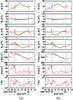 |
Fig. 1 Magnetic cloud of April 22, 2001. Observations (5-min averages) are plotted by the red lines, B, Bx, By, and Bz are the magnetic field magnitude and the field components in the GSE coordinates, V, N, and T are the solar wind velocity, proton number density, and proton temperature, respectively. Estimated cloud boundaries are drawn by the blue vertical lines. The thick green lines are fits by cylindrical models, namely a) the (spatially) constant-α force-free field (the Lundquist solution) with expansion, and b) (spatially) uniform-twist field (the Gold-Hoyle tube) with expansion. |
They are successfully locally modeled almost from the beginning by the axially symmetric constant-α force-free cylindrical magnetic field found by Lundquist (1950) (Burlaga 1988; Lepping et al. 1990, 2006), which in cylindrical coordinates r, ϕ, and z reads
 where J0 and J1 are the Bessel functions of the first kind, B0 is the maximum magnetic field magnitude, and α is a constant fulfilling
  (4)The α is related to the flux-rope radius r0 by
  (5)where a0 is the first root of J0 (J0(a0) = 0, a0 ≐ 2.41). The sign stands for chirality, a plus means a right-handed flux rope. This selection of α yields the axial field Bz = 0 at the flux rope boundary.
Magnetic clouds expand during their propagation (Klein & Burlaga 1982), which is manifested by an almost linear decrease of the solar wind velocity magnitude (Fig. 1). The first attempts to incorporate expansion into models of magnetic clouds were made by Osherovich et al. (1993) and Marubashi (1997). Analytical solutions of an expanding cylindrical flux rope (Shimazu & Vandas 2002; Berdichevsky et al. 2003) indicate that they can asymptotically be described by Eqs. (1)–(3) with time-dependent B0 and α, meaning that the fields are spatially force-free and ![Mathematical equation: \begin{eqnarray} && B_0 = B_{00} [1+E (t-t_0)]^{-2}, \label{B0t} \\ && \alpha = \alpha_0 [1+E (t-t_0)]^{-1}, \label{alt} \end{eqnarray}](/articles/aa/full_html/2017/12/aa31412-17/aa31412-17-eq24.png) where E is the expansion factor, t is the time, and B00 and α0 are quantities at t = t0 (for our purposes, t0 is the time when a spacecraft enters a flux rope or magnetic cloud). It follows from the definition of α by Eq. (5) that the flux rope radius rt increases linearly in time,
where E is the expansion factor, t is the time, and B00 and α0 are quantities at t = t0 (for our purposes, t0 is the time when a spacecraft enters a flux rope or magnetic cloud). It follows from the definition of α by Eq. (5) that the flux rope radius rt increases linearly in time, ![Mathematical equation: \begin{equation} r_t = r_0 [1+E (t-t_0)], \label{rt} \end{equation}](/articles/aa/full_html/2017/12/aa31412-17/aa31412-17-eq32.png) (8)and that
(8)and that  (9)We can also obtain these time dependencies heuristically, assuming that the flux rope expansion is given by Eq. (8). The magnetic flux of the flux rope must be conserved during expansion. The flux through its cross section is for the field (1)–(3) given by
 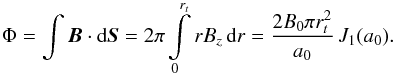 (10)We see that Φ is independent of time when B0 behaves as given by Eq. (6).
Figure 1a shows an observation of a magnetic cloud identified by Lepping et al. (2006) and its fit by the model (1)–(3) when expansion is considered. All observations presented in this paper were taken from OMNIWeb through the Space Physics Data Facility at NASA GSFC. The fitting procedure is described in detail in Vandas et al. (2015), and it yields the flux rope orientation, radius, impact parameter (signed closest approach to the rope axis divided by r0), flux rope velocity, and expansion factor. Fitted are the magnetic field components and the velocity magnitude. The resulting geometric parameters in our case are r0 = 0.10 AU, ϑ = − 56° (inclination angle to the ecliptic plane in the geocentric solar ecliptic (GSE) coordinates), φ = 269° (azimuthal angle in the ecliptic plane in the GSE coordinates), and p = − 0.09 (impact parameter); the field is left-handed.
Magnetic field lines in flux ropes are helically twisted around its magnetic axis. The angle that a magnetic field line makes around the axis and along it within a unit length is called its twist per unit length. For the Lundquist solution (1)–(3), the twist of magnetic field lines approaching the boundary increases without limits because Bz goes to zero while | Bϕ | increases (cf. Fig. 8). However, investigations indicate that interplanetary magnetic flux ropes (magnetic clouds) have a relatively weak twist, contrary to the Lundquist solution (Larson et al. 1997; Hu et al. 2014, 2015). In principle, we could suppress the strong twist in the Lundquist solution by a selection of a smaller flux rope radius than r0 given by Eq. (5) (for a fixed α following from a fit), because every r = const. is a magnetic surface (due to Br = 0). Another problem would emerge, however: the magnetic field magnitude profile would be too shallow, contrary to observations. It is therefore suggested that a uniform-twist model might be more relevant (Hu et al. 2015).
The magnetic field of a cylindrical flux rope with a uniform twist (the so-called Gold-Hoyle tube, Gold & Hoyle 1960) is given by 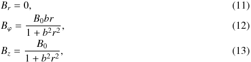 where b is a parameter related to the twist and its sign gives the field chirality, and B0 determines the level of the magnetic field magnitude. It is a nonlinear force-free field with
 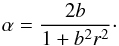 (14)The twist per unit length is given by
 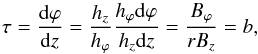 (15)and it is constant. The Lamé coefficients for cylindrical coordinates are hϕ = r and hz = 1. As in the case of the Lundquist solution, Br = 0, therefore every r = const. may serve as a flux rope boundary. In contrast to the Lundquist solution, Bz does not change its sign.
Farrugia et al. (1999) were the first to fit a particular magnetic cloud with this solution. Recently, Wang et al. (2016) made a comprehensive study and fit many magnetic clouds by the Gold-Hoyle field (11)–(13). The authors included expansion of flux ropes in a manner similar to that described above for the Lundquist solution. Following the heuristic approach, it is again assumed that the flux rope expands according to Eq. (8). The magnetic flux through the rope cross section is  (16)Φ is independent of time when B0 behaves as given by Eq. (6) and b by
 ![Mathematical equation: \begin{equation} b = b_0 [1+E (t-t_0)]^{-1}, \label{bt} \end{equation}](/articles/aa/full_html/2017/12/aa31412-17/aa31412-17-eq52.png) (17)where b0 is the value of b at t = t0. Similarly to Eq. (9), it holds
(17)where b0 is the value of b at t = t0. Similarly to Eq. (9), it holds  (18)Figure 1b shows the same observation of the magnetic cloud as Fig. 1a, but supplemented with a fit by the uniform-twist model (11)–(13) when expansion is considered. The fitting algorithm was the same as in the previous case. The resulting geometric parameters now are r0 = 0.07 AU, ϑ = − 34°, φ = 207°, and p = 0.44; the unit-less twist is b0r0 = − 2.1. We see from Fig. 1 that the uniform-twist field fits the observations equally well as the constant-α field. However, the parameters differ, notably the impact parameter.
In some cases of magnetic cloud observations, a local approximation by a cylindrical flux rope is not appropriate because the curvature of the flux rope plays a role. Some approximate variants of the Lundquist solution in toroidal geometry have been used to fit these observations (Marubashi 1997; Marubashi & Lepping 2007). There are also other toroidal solutions found in space-physics literature, for instance, an approximately force-free field with a uniformly distributed toroidal current by Titov & Démoulin (1999), applied to coronal flux ropes, or a non-force-free field in a loop-like flux rope with varying cross section by Hidalgo (2014), applied to magnetic cloud observations. Recently, a procedure suggesting a Grad-Shafranov reconstruction of magnetic fields in toroidal flux ropes has been proposed (Hu 2017). It assumes rotational symmetry, static structure, and an arbitrary cross section. In view of the current preference for weak-twist solutions, we question such solutions in toroidal geometry. More specifically, in the present paper, we search analytically for an analog of the Gold-Hoyle field (11)–(13) for a toroidal flux rope, that is, a uniform-twist field in an ideal toroid.
The paper is organized as follows: in Sect. 2 we derive three solutions of (nearly) uniform-twist magnetic fields in an ideal toroid of arbitrary aspect ratio, which are exactly solenoidal and approximately force-free (with an increasing accuracy). Section 3 presents fits of a magnetic cloud by the toroidal solutions, and Sect. 4 concludes the paper. The magnetic cloud was taken from the list by Marubashi & Lepping (2007), and our fitting approach closely follows the cited paper. We investigated the performance of the solutions in comparison with the known constant-α force-free field in context of the results by Marubashi & Lepping (2007).
2. Construction of (nearly) uniform-twist magnetic fields in an ideal toroid
Uniform-twist toroidal flux ropes can be constructed quite easily. We work in toroidally curved cylindrical coordinates, r, ϕ, and θ, where  These coordinates describe an ideal toroid with the major radius R0, minor radius r0, and the rotational axis coinciding with the z-axis, by r ∈ ⟨ 0,r0 ⟩, ϕ ∈ ⟨0,2π), and θ ∈ ⟨0,2π); r = r0 is the equation of the toroid boundary.
In accord with Eqs. (11)–(13), we assume that the field is azimuthally symmetric and set  (22)which means that magnetic surfaces are symmetrically coaxial toroids. The magnetic field lines helically wind on toroids, and their constant twist means the condition
  (23)where hϕ = R0 + rcosθ and hθ = r are the Lamé coefficients. The third condition is
  (24)which is simply
  (25)We may therefore write
  (26)where F is a function. From Eq. (23) we have
  (27)However, this field cannot be strictly force-free because of Eq. (22).
When we require that the field with the components (22), (27), and (26) tend to the Gold-Hoyle field (11)–(13) for high aspect ratios, then τ and F are determined, and we have  We call this the uniform-twist field in the paper.
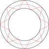 |
Fig. 2 Toroidal flux rope with a uniform-twist field. One magnetic field line is drawn in red. It closes in on itself, and this holds for all field lines. This behavior only occurs for specific values of twist, otherwise the field lines are ergodic. |
For specific values of twist, all magnetic field lines are closed, that is, if 2πbR0 = n, where n is an integer. One such field line is shown in Fig. 2. Figure 3 shows a cross section of a flux rope with the field given by Eqs. (28)–(30). We see that the magnetic field magnitude maximum is shifted toward the toroid hole from the toroid circular axis, and that such a flux rope will be approximately force-free only for very high aspect ratios.
We note that Chui & Moffatt (1992) derived another uniform-twist field in an ideal toroid. In their case, τ from Eq. (23) is not constant, but all field lines make the same number of turns along the whole toroid. We may therefore say that the integral twist is constant for this field, while in our case, the differential twist is constant. However, their solution has a minimum of the magnetic field magnitude inside the rope and the magnitude increases toward the boundary, which means that this field is not suitable for modeling of magnetic clouds.
The question is whether the cylindrical field (11)–(13) can be generalized to a toroidal field that would represent a toroidal flux rope with an (approximately) uniform twist and an (approximately) force-free field. We search for an approximate solution in such a way that the field (11)–(13) is taken as a zero-order solution and corrections on the order of r/R0 (r ≤ r0) are evaluated. For the constant-α Lundquist solution, this procedure yields the Miller & Turner (1981) solution cut at  , explicitly,
 ![Mathematical equation: \begin{eqnarray} && B_r = B_0 J_0(\alpha r) \frac{\sin \theta}{2 \alpha R_0}, \label{BrMT} \\ && B_\varphi = B_0 J_0(\alpha r) \left(1-\frac{r \cos \theta}{2 R_0}\right), \label{BpMT} \\ && B_\theta = -B_0 \left\{J_1(\alpha r)-\left[J_0(\alpha r)+ \alpha r J_1(\alpha r)\right] \frac{\cos \theta}{2 \alpha R_0}\right\}\cdot \label{BtMT} \end{eqnarray}](/articles/aa/full_html/2017/12/aa31412-17/aa31412-17-eq83.png) We call this the MT solution. It is approximately solenoidal and approximately force-free (Vandas & Romashets 2015). For α given by Eq. (5), the boundary of the ideal toroid with r0 and R0 is a magnetic surface where Br = 0. In addition, Bϕ = 0 there as well, which means that the field is purely poloidal and the twist of the magnetic field lines goes to infinity there, similarly as for the Lundquist solution (cf. Fig. 8).
We call this the MT solution. It is approximately solenoidal and approximately force-free (Vandas & Romashets 2015). For α given by Eq. (5), the boundary of the ideal toroid with r0 and R0 is a magnetic surface where Br = 0. In addition, Bϕ = 0 there as well, which means that the field is purely poloidal and the twist of the magnetic field lines goes to infinity there, similarly as for the Lundquist solution (cf. Fig. 8).
An azimuthally symmetric toroidal force-free field in toroidally curved cylindrical coordinates must fulfill ![Mathematical equation: \begin{eqnarray} && -\frac{1}{r h_\varphi} \frac{\partial}{\partial \theta} (h_\varphi B_\varphi) = \alpha B_r, \label{Bre5} \\ && \frac{1}{r} \left[\frac{\partial B_r}{\partial \theta} - \frac{\partial}{\partial r} (r B_\theta)\right] = \alpha B_\varphi, \label{Bpe5} \\ && \frac{1}{h_\varphi} \frac{\partial}{\partial r} (h_\varphi B_\varphi) = \alpha B_\theta, \label{Bte5} \\ && r B_r \frac{\partial \alpha}{\partial r}+ B_\theta \frac{\partial \alpha}{\partial \theta} = 0. \label{div5} \end{eqnarray}](/articles/aa/full_html/2017/12/aa31412-17/aa31412-17-eq85.png) These equations are explicitly written in conditions (4) and (24), respectively. Inserting the components Br and Bθ from Eqs. (34) and (36) into Eqs. (35) and (37), we obtain
These equations are explicitly written in conditions (4) and (24), respectively. Inserting the components Br and Bθ from Eqs. (34) and (36) into Eqs. (35) and (37), we obtain ![Mathematical equation: \begin{eqnarray} && \frac{\partial}{\partial \theta} \left[ \frac{1}{\alpha r h_\varphi} \frac{\partial}{\partial \theta} (h_\varphi B_\varphi) \right] + \frac{\partial}{\partial r} \left[ \frac{r}{\alpha h_\varphi} \frac{\partial}{\partial r} (h_\varphi B_\varphi) \right] + \alpha r B_\varphi = 0, \label{Bpe5a} \\ && \frac{\partial \alpha}{\partial r} \frac{\partial}{\partial \theta} (h_\varphi B_\varphi) - \frac{\partial \alpha}{\partial \theta} \frac{\partial}{\partial r} (h_\varphi B_\varphi) = 0. ~~~~~~~~~~~~~~~~~~~~~~~~~~~~~~~~~~~~~~~~~~ \label{div5a} \end{eqnarray}](/articles/aa/full_html/2017/12/aa31412-17/aa31412-17-eq88.png) Equation (39) is fulfilled when
Equation (39) is fulfilled when  (40)where
  is a function. From analogy with the cylindrical solution (11)–(14), it follows
  (41)We may therefore set
  (42)In this case, Eq. (39) is fulfilled, which means that the field is exactly solenoidal. The components Br and Bθ are given by Eqs. (34) and (36) from Bϕ, therefore the force-free condition is fulfilled for them exactly. Equation (38) yields
  (43)which is an equation for α. We rewrite it in the form
  (44)We solve this approximately by setting α = αc(r)(1 + δα1), where αc is given by Eq. (14) (from the cylindrical solution, but r is now interpreted as the toroidal coordinate r) and δα1(r,θ) is on the order of .
 |
Fig. 3 a) Magnetic field magnitude distribution and b) distribution of angles δ between the field vectors and current for a toroidal flux rope with aspect ratio R0/r0 = 5, uniform-twist field, and unit-less twist br0 = 1.5. Lines are cross sections of magnetic field surfaces on which magnetic field lines lie. The thick line (circle) is the flux rope boundary. The magnetic field magnitude B is scaled by its maximum value Bmax inside the flux rope. The angle δ is zero for an exact force-free solution. |
When we set δα1 = 0, the zero-order terms in Eq. (35) cancel as expected, but the terms remain. This means that Eq. (44) is fulfilled as 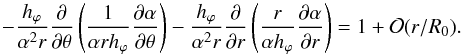 (45)Components follow from Eqs. (34), (42), and (36) with α = αc, and they are
  These equations determine a solenoidal solution for a toroidal flux rope with a circular cross section. It is approximately force-free only for high aspect ratios, or near the flux rope magnetic axis (flux rope core) where r is small. It has an approximately uniform twist (given by b). For brevity, this field is called the zero-order solution in the paper.
For δα1 ≠ 0, we try to meet Eq. (44) to first order, that is,  (49)Setting δα1 = α1(r,θ) r/R0, where α1 is on the order of
  , we obtain from condition (49) an equation for α1:
  (50)The prime means derivative by r and the dot by θ. There is a term with cosθ and terms with α1, its derivatives by r, and terms with
  . We may therefore set α1 = f1(r)cosθ to meet the theta dependence. We obtain from Eq. (50)
  (51)The solution of Eq. (51) is given in Appendix A. It depends on a parameter that may be a value of f1(0).
Knowing the function f1(r), we can evaluate the field components: ![Mathematical equation: \begin{eqnarray} && B_r = \frac{B_0 R_0 f_1(r) \sin \theta}{2 b (R_0+r \cos \theta) [R_0+r f_1(r) \cos \theta]},~~~~~~~~~~~~~~~~~~~~~~~~~~~~~~~ \label{Br6} \\ && B_\varphi = \frac{B_0 [R_0+r f_1(r) \cos \theta]}{(1+b^2 r^2) (R_0+r \cos \theta)},~~~~~~~~~~~~~~~~~~~~~~~~~~~~~~~~~~~~~~~~~~~ \label{Bp6} \\ && B_\theta = B_0 R_0 [(1-b^2 r^2) f_1(r) \cos \theta+(1+b^2 r^2) r f_1^\prime(r) \cos \theta \nonumber \\ & &\qquad -\,2 b^2 r R_0] ~~~~~~~~~~~~~~~~~~~~~~~~~~~~~~~~~~~~~~~~~~~~~~~~~~~~~~~~~~~~~~~~~~~~\nonumber \\ & &\qquad \times \, \big\{2 b (1+b^2 r^2) (R_0+r \cos \theta) [R_0+r f_1(r) \cos \theta]\big\}^{-1}, ~~~~~~~~~~~~~~~~~~~~~~~~~~~~~~~ \label{Bt6} \end{eqnarray}](/articles/aa/full_html/2017/12/aa31412-17/aa31412-17-eq119.png) α is
α is ![Mathematical equation: \begin{equation} \alpha = \frac{2 b [R_0+r f_1(r) \cos \theta]}{(1+b^2 r^2) R_0}\cdot \label{al6} \end{equation}](/articles/aa/full_html/2017/12/aa31412-17/aa31412-17-eq120.png) (55)Equations (52)–(54) determine a solenoidal solution for a toroidal flux rope that has a circular cross section when the value of f1(0) is properly chosen (as described in Appendix A). It is approximately force-free, on the order of
(55)Equations (52)–(54) determine a solenoidal solution for a toroidal flux rope that has a circular cross section when the value of f1(0) is properly chosen (as described in Appendix A). It is approximately force-free, on the order of  , and with an approximately uniform twist (given by b). This field is called the first-order solution in the paper for brevity.
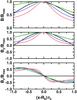 |
Fig. 4 Magnetic field profiles along the x axis for several flux ropes with R0/r0 = 5. Comparison of the MT solution (black lines) to the zero-order solution with several values of br0. The green lines are for br0 = 1, the blue lines for br0 = 2, and the red lines for br0 = 3. |
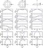 |
Fig. 5 Magnetic field profiles for four flux ropes and along three different directions are shown in the middle part. Comparison of the MT solution (in black) to the zero- (in green) and first- (in red) order solutions and the uniform-twist solution (in blue). All flux ropes have circular cross sections with radius r0, R0/r0 = 5, and br0 = 1.5. Trajectories along which the profiles are displayed are shown by the thick arrows in the top sketches of the flux ropes. Panel a displays the profiles along the x-axis, panel b along the line parallel to the y-axis and crossing the x-axis at the point [R0−r0/ 2,0,0], and panel c along the line parallel to the z-axis and crossing the x-axis at the point [R0,0,0]. The bottom part shows hodograms of the magnetic field vectors along the displayed trajectories. The color coding of the lines is the same as in the middle part. The arrows show directions of the hodograms and also indicate the entry into the toroid (blue) and the exit (green). |
Figure 4 shows profiles of the magnetic field magnitude and components for several toroidal flux ropes with R0/r0 = 5. The Bx component at the x-axis is the radial field, which is exactly zero for all solutions and therefore not shown; the By component is the axial field, and the Bz component is the azimuthal field. The constant-α MT field is plotted with the black line for reference. Its axial field reaches zero at the boundary (this indicates infinite twist), while the other fields do not, which are the zero-order solutions with different twist parameters b. We see that the best correspondence to the MT solution is br0 between 1 and 2. Therefore Fig. 5 is made for br0 = 1.5. The MT and zero-order solutions are given by the black and green lines, respectively. The red lines show profiles of the first-order solution, and the blue lines show profiles of the uniform-twist solution. The value of f1(0) for the first-order solution was determined by the condition f1(r0) = 0, as described in Appendix A. We see that the differences among the first- and zero-order solutions and the uniform-twist solution are very small, one profile often obscures another in the panels. The MT solution matches the other solutions in the Bz component and the inner part (r/r0 ≲ 0.5) in the Bx and By components.
Figures 6–7 show flux ropes with zero- and first-order solutions and for two aspect ratios, 5 and 3, respectively. The Cartesian coordinate system is the same as in figures displaying profiles (i.e., Figs. 4–5). Lines are cross sections of magnetic surfaces with the plane y = 0. They are circular for the top panels and nearly circular for the bottom panels. The angle δ in the figures tests the force-free condition. We see that the first-order solution strongly improves it.
We determined the twist of magnetic field lines by tracing them along the toroid and counting their turns. The twist per unit length was then calculated by dividing the twist by the toroid length. It is denoted as  to distinguish it from τ defined by Eq. (23), which depends on spatial coordinates (e.g., θ) and changes along a field line. The results are shown in Fig. 8. Twists per unit length are nearly constant and close to b. The zero-order solution is closer to the value of b than the first-order solution, but the differences are small. For lower aspect ratios, the twist has larger deviations from b near the flux rope boundary and it is decreasing. The uniform-twist solution, Eqs. (28)–(30), would clearly have τ equal to b, and it would be represented by the horizontal dashed line in the figure.
3. Fit of a magnetic cloud observation by toroidal models
Marubashi & Lepping (2007) analyzed long-duration magnetic clouds and fit them by a toroidal model similar to the MT solution. We took one cloud from their list, namely the magnetic cloud of March 19–22, 2001 (their event 13), and fit its observation by the MT field and the toroidal fields derived in this paper to determine whether the resulting fits have a similar quality as in the case of the fits by cylindrical models presented in the Introduction.
To do this, we first incorporated expansion into the field equations. We followed the way described in the Introduction. The toroidal flux rope has a major radius Rt and a minor radius rt at a time t. It is again assumed that rt behaves according to Eq. (8).
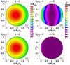 |
Fig. 6 Magnetic field magnitude distribution (a, c) and distribution of angles δ between the field vectors and current (b, d) for a toroidal flux rope with aspect ratio R0/r0 = 5 given by the zero-order solution in the top panels (a, b), and by the first-order solution in the bottom panels (c, d). The lines are cross sections of magnetic field surfaces on which magnetic field lines lie. The thick line (circle) is the flux rope boundary. It is br0 = 1.5. |
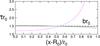 |
Fig. 8 Twist |

For the MT field, α must fulfill Eq. (7) in order for the expanding toroid to be a magnetic surface according to Eq. (31). The magnetic flux through the flux-rope cross section (toroidal flux) is given by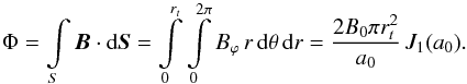 (56)Bϕ is taken from Eq. (32) with R0 replaced by Rt. We obtained the same expression as for the Lundquist solution, Eq. (10). This means that B0 must behave as given by Eq. (6) for the magnetic flux to be conserved. The magnetic helicity of the flux rope should also be conserved during expansion, it is approximately given (Vandas & Romashets 2015) by
 ![Mathematical equation: \begin{equation} H = \frac{B_0^2 \pi^2 r_t^3 R_t}{2 a_0} \left[8-\left(1+\frac{1}{a_0^2} \right) \frac{r_t^2}{R_t^2}\right] {J}_1^2(a_0) \, \mathrm{sign} \, \alpha, \label{HMT} \end{equation}](/articles/aa/full_html/2017/12/aa31412-17/aa31412-17-eq139.png) (57)where the sign is the signum function (the helicity is approximate because the field itself is only approximately solenoidal). It follows from this formula that H is independent of time when the aspect ratio Rt/rt is constant, in other words, Rt behaves similarly to rt, Rt = R0 [1 + E(t−t0)].
(57)where the sign is the signum function (the helicity is approximate because the field itself is only approximately solenoidal). It follows from this formula that H is independent of time when the aspect ratio Rt/rt is constant, in other words, Rt behaves similarly to rt, Rt = R0 [1 + E(t−t0)].
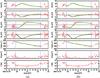 |
Fig. 9 Magnetic cloud of March 19–22, 2001. The format of the figure is the same as Fig. 1. The thick green lines are fits by toroidal models, namely a) the MT field with expansion, and b) the zero-order solution with expansion. |
For the uniform-twist field, the toroidal flux coincides with formula (16) for the cylindrical case, which means that when b and B0 meet Eqs. (17) and (6), the flux is conserved. To calculate the helicity of the uniform-twist field, the formula by Berger (1998) can be used, which holds for an axially symmetric toroidal flux rope that consists of a set of nested magnetic surfaces, 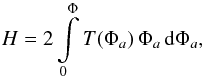 (58)where Φa is the axial (toroidal) magnetic flux within a particular magnetic surface, Φ is the total axial flux, that is, Φa of the outermost surface (boundary). T(Φa) is the number of field-line turns about the magnetic axis at the magnetic surface labeled by Φa. In our case, T = bRt, Φ is given by Eq. (16), and the integral (58) can be immediately evaluated,
 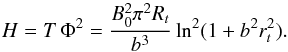 (59)As in the previous case, H does not depend on time when the aspect ratio remains constant.
With the last equation, the helicity per unit length can be determined, 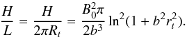 (60)The formula coincides with the relative helicity per unit length for the cylindrical uniform-twist flux rope, calculated by Dasso et al. (2003), which is used to characterize the helicity of cylindrical flux ropes (Dasso et al. 2003; Wang et al. 2016).
The toroidal magnetic flux of the toroidal rope with the zero-order solution is also given by Eq. (16) and the helicity has a more complex formula, which is given in Appendix B. They are conserved when the parameters behave as in the case of the uniform-twist field. The same is true for the first-order solution. Here we do not derive analytical formulae for the magnetic flux and helicity, but a close inspection of their integral representations confirms this statement.
Fit parameters for the toroidal models.
Figure 9 shows the observation of the magnetic cloud of March 19–22, 2001. In order to fit it by the toroidal fields from Sect. 2, we exactly followed the geometric model of a toroidal flux rope given by Marubashi & Lepping (2007). The only difference was that we used other magnetic fields and another fitting procedure. The list of model parameters is the following. The toroid has a major radius R0 and a minor radius r0 at a spacecraft entry (at time t0). The minor radius expands according to Eq. (8), so that the expansion factor E belongs to the parameter set. The major radius is kept constant, Rt = R0, otherwise the geometrical calculations would be very complicated, as the authors note. This somewhat contradicts the conservation of magnetic helicity (see above), but we can expect that the results are not greatly affected (the change in Rt is not very large). The toroid rotational-axis direction is determined by the inclination angle ϑn and the azimuthal angle φn in the GSE system. The angles are kept constant in time. The toroid as a whole moves with a velocity U = U0−D(t−t0) along the xGSE-axis. U0 and D are parameters of the model. The deceleration D had to be introduced (Marubashi & Lepping 2007) so that the velocity magnitude inside magnetic clouds was satisfactorily matched (unlike in the cylindrical model, where this is not necessary). The resulting velocity inside the toroidal flux rope (magnetic cloud) is the vector sum of U and the expansion radial velocity vr = Er [1 + E(t−t0)] -1. Two impact parameters py and pz define the spacecraft trajectory relative to the toroid axis (for details see Marubashi & Lepping 2007). The level of the magnetic field magnitude is given by B00 and the field twist by α0 or b0; while α0 is firmly given by Eq. (5), b0 is a free parameter. Because E can be calculated from the other parameters, there are nine free parameters of the model for the MT field, and ten free parameters for the other toroidal fields. The sign of α0 or b0 (chirality) is given at the beginning of our fitting procedure (by trial and error) and the unit-less quantity Δ,  is minimized using the nonlinear least-squares method by Powell (Press et al. 2002; Vandas et al. 2015). The superscript (o) means observed values, while (m) denotes modeled values, NB is the number of the magnetic field B measurements, NV is the number of the solar wind velocity V measurements, Bmax and Vmax their maximum magnitude values. The weights were set wB = wV = 0.5. The quantity ΔB is equal to Erms listed by Marubashi & Lepping (2007).
We note that exactly the same fitting procedure was used for the fits presented in the Introduction (Fig. 1), only a simpler model (cylinder) was used (and of course the cylindrical fields), with three free parameters less (D and R0 are not involved, and instead of two parameters py and pz, only one p is involved).
In addition to observations, Fig. 9 shows fits of them by two toroidal models, with the MT and the zero-order solutions. The fits have a comparable quality. We took the same time interval of the event as Marubashi & Lepping (2007) did and 5-min data; this represented NB = 669 and NV = 665 observational points (some measurements were missing). As the initial values for the fitting procedure, we entered the values obtained by Marubashi & Lepping (2007). They are listed in Table 1 together with values from our fits for four toroidal models. The flux rope was left-handed (i.e., the values of α0 and b0 are negative).
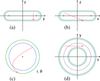 |
Fig. 10 Trajectory of a spacecraft (red arrows) through the model of the expanding toroidal flux rope, corresponding to the fit from Fig. 9b. The trajectory is shown in the intrinsic Cartesian system x, y, and z of the toroid, Eqs. (19)–(21) (the coordinates are different from the GSE coordinates), in projection to the a) yz-plane, b) xz-plane, and d)xy-plane; panel c displays the trajectory in a cross section of the toroid, where coordinates r and θ serve as polar coordinates. The blue lines are the boundaries of the toroid at the spacecraft entry, the green lines are the boundaries at the exit. According to the model assumptions, the minor radius of the toroid increases during expansion, while the major radius remains constant. |
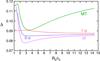 |
Fig. 11 Δ as a function of the aspect ratio for four magnetic field solutions: the uniform-twist field (ut, magenta), the zero-order solution (0-o, blue), the first-order solution (1-o, red), and the MT field (MT, green). The values of Δ are approximately one half of the ΔB values because the values of ΔV are small, see Eq. (61). |
The parameters from the fit by the MT field are similar to the values by Marubashi & Lepping (2007). This corresponds to the fact that both models are quantitatively similar. The uniform-twist and the zero-order solutions also yield parameters that are not very far from these values. We expected that the same would hold for the first-order solution, which is only a small correction to the zero-order case. To our surprise, the parameters are very different (see Table 1), mainly the values of the toroid radii and aspect ratio. On the other hand, the quality of the fit represented by ΔB is comparable to the other fits. Figure 9b shows the fit by the zero-order solution, but the fits by the uniform-twist field as well as by the first-order solution are nearly the same and are therefore not shown. Figure 10 displays the trajectory of the spacecraft through an expanding toroidal cloud according to the model with the zero-order solution. Trajectories are similar in the other models, including the first-order solution; but in the latter case, the toroid would be very thin.
In order to determine the reason for this difference in parameters, we examined the dependence of Δ on the aspect ratio. This dependence is shown in Fig. 11. To determine Δ, a modified fitting procedure was used, where the aspect ratio was kept constant, that is, the number of free parameters was one less. The displayed Δ is the resulting Δ from the fitting procedure (minimum Δ found). The zero- and first-order solutions do not have a well-expressed minimum in Δ, their Δ is nearly constant for a wide range of aspect ratios. The uniform-twist field behaves better in this respect, and the MT field has the best-expressed Δ-minimum. It follows that geometric parameters may not be reliably determined for (nearly) uniform-twist flux ropes in some cases, especially the toroid radii and aspect ratio (and consequently py and pz).
4. Conclusions
We derived three solutions of (nearly) uniform-twist magnetic fields in an ideal toroid, which may serve as models of low-twist fields. All are exactly solenoidal, and in the limit of high aspect ratios, they tend to the Gold-Hoyle field (i.e., a nonlinear uniform-twist force-free field). The first solution is far from a force-free field for moderate aspect ratios, but it is exactly a uniform-twist field. The other two fields have a nearly uniform twist and approximate force-free fields, they are two subsequent solutions in accuracy, which involves the value of aspect ratio.
When crossings of a hypothetic spacecraft through a toroidal flux rope are simulated, all three solutions yield very similar magnetic field profiles. This means that they can be alternatively involved in fitting procedures, or they can test the robustness of the fitting when used subsequently.
We analyzed the magnetic cloud observation during April 19–22, 2001. We fit the observed data by the known approximately linear force-free field in a toroid (Miller-Turner field) and by the newly derived toroidal fields. In our fitting procedure, we followed a traditional way (Lepping et al. 1990, 2006; Marubashi & Lepping 2007; Vandas et al. 2015) and evaluated the quality of the fit by the value of ΔB and by eye inspection. Fits by all models had a comparable quality. However, this analysis also revealed that the geometric parameters of the toroid following from the fit might not be reliably determined when (nearly) uniform-twist model fields are used. Sets of parameterslargely differing in the size of the toroid and its aspect ratio yield fits of a comparable quality. Usage of more models and their intercomparison may suppress this ambiguity.
Acknowledgments
We acknowledge the use of data from OMNIWeb (NASA/GSFC/SPDF) and the PIs who provided them. This work was supported by project 17-06065S from GA ČR and by the AV ČR grant RVO:67985815.
References
- Abramowitz, M., & Stegun, I. A. 1972, Handbook of Mathematical Functions with Formulas, Graphs, and Mathematical Tables, 9th printing (Mineola, NY: Dover Publications) [Google Scholar]
- Berdichevsky, D., Lepping, R. P., & Farrugia, C. J. 2003, Phys. Rev. E, 67, 036405 [NASA ADS] [CrossRef] [Google Scholar]
- Berger, M. A. 1998, in New Perspectives on Solar Prominences, IAU Colloq., 167, eds. D. Webb, D. Rust, & B. Schmieder (San Francisco: ASP), ASP Conf. Ser., 150, 102 [Google Scholar]
- Burlaga, L. F. 1988, J. Geophys. Res., 93, 7217 [NASA ADS] [CrossRef] [Google Scholar]
- Burlaga, L., Sittler, E., Mariani, F., & Schwenn, R. 1981, J. Geophys. Res., 86, 6673 [Google Scholar]
- Chui, A. Y. K., & Moffatt, H. K. 1992, in Topological Aspects of the Dynamics of Fluids and Plasmas, eds. H. K. Moffatt, G. M. Zaslavsky, P. Comte, & M. Tabor (Dordrecht, The Netherlands: Kluwer Academic Publishers), NATO ASI Series, 195 [Google Scholar]
- Dasso, S., Mandrini, C. H., Démoulin, P., & Farrugia, C. J. 2003, J. Geophys. Res., 108, 1362 [NASA ADS] [CrossRef] [Google Scholar]
- Farrugia, C. J., Janoo, L. A., Tobert, R. B., et al. 1999, in Solar Wind Nine, eds. S. R. Habbal, R. Esser, J. V. Hollweg, & P. A. Isenberg (Woodbury, New York: AIP), AIP Conf. Proc., 471, 745 [Google Scholar]
- Gold, T., & Hoyle, F. 1960, MNRAS, 120, 89 [NASA ADS] [Google Scholar]
- Hidalgo, M. A. 2014, ApJ, 784, 67 [NASA ADS] [CrossRef] [Google Scholar]
- Hu, Q. 2017, Sol. Phys., 292, 116 [NASA ADS] [CrossRef] [Google Scholar]
- Hu, Q., Qiu, J., Dasgupta, B., Khare, A., & Webb, G. M. 2014, ApJ, 793, 53 [NASA ADS] [CrossRef] [Google Scholar]
- Hu, Q., Qiu, J., & Krucker, S. 2015, J. Geophys. Res., 120, 5266 [Google Scholar]
- Klein, L. W., & Burlaga, L. F. 1982, J. Geophys. Res., 87, 613 [Google Scholar]
- Krimigis, S., Sarris, E., & Armstrong, T. 1976, Trans. AGU, 57, 304 [Google Scholar]
- Larson, D. E., Lin, R. P., McTiernan, J. M., et al. 1997, Geophys. Res. Lett., 24, 1911 [NASA ADS] [CrossRef] [Google Scholar]
- Lepping, R. P., Jones, J. A., & Burlaga, L. F. 1990, J. Geophys. Res., 95, 11957 [NASA ADS] [CrossRef] [Google Scholar]
- Lepping, R. P., Berdichevsky, D. B., Wu, C.-C., et al. 2006, Ann. Geophys., 24, 215 [NASA ADS] [CrossRef] [Google Scholar]
- Lundquist, S. 1950, Ark. Fys., 2, 361 [Google Scholar]
- Marubashi, K. 1997, in Coronal Mass Ejections, eds. N. Crooker, J. Joselyn, & J. Feyman (Washington, DC: AGU), Geophys. Monogr. Ser., 99, 147 [Google Scholar]
- Marubashi, K., & Lepping, R. P. 2007, Ann. Geophys., 25, 2453 [NASA ADS] [CrossRef] [Google Scholar]
- Miller, G., & Turner, L. 1981, Phys. Fluids, 24, 363 [NASA ADS] [CrossRef] [Google Scholar]
- Osherovich, V. A., Farrugia, C. J., & Burlaga, L. F. 1993, Adv. Space Res., 13(6), 57 [NASA ADS] [CrossRef] [Google Scholar]
- Press, V. H., Teukolsky, S. A., Vetterling, W. T., & Flannery, B. P. 2002, Numerical Recipes in C, The Art of Scientific Computing, 2nd edn. (New York: Cambridge University Press) [Google Scholar]
- Shimazu, H., & Vandas, M. 2002, Earth Planets Space, 54, 783 [NASA ADS] [CrossRef] [Google Scholar]
- Titov, V. S., & Démoulin, P. 1999, A&A, 351, 707 [NASA ADS] [Google Scholar]
- Vandas, M., & Romashets, E. 2015, A&A, 580, A123 [NASA ADS] [CrossRef] [EDP Sciences] [Google Scholar]
- Vandas, M., Romashets, E., & Geranios, A. 2015, A&A, 583, A78 [NASA ADS] [CrossRef] [EDP Sciences] [Google Scholar]
- Wang, Y., Zhuang, B., Hu, Q., et al. 2016, J. Geophys. Res., 121, 9316 [CrossRef] [Google Scholar]
Appendix A: Analytical expression for f1
Equation (51) with the substitution s = (br)2 is transformed into  (A.1)where the primes are derivatives by s. This equation is further rewritten using the substitution t = 1/(1 + s),
  (A.2)where now the primes are derivatives by t. The homogeneous part of this equation has a solution t. Setting f1(t) = tg1(t) in Eq. (A.2) yields
  (A.3)The homogeneous part of this equation has a solution [t(1−t)] -2 with respect to
  . We set
 ![Mathematical equation: \hbox{$g_1^\prime(t)=[t (1-t)]^{-2} \tilde{g}_1(t)$}](/articles/aa/full_html/2017/12/aa31412-17/aa31412-17-eq250.png) in Eq. (A.3) and obtain the equation
in Eq. (A.3) and obtain the equation  (A.4)which has the solution
  (A.5)where C2 is an integration constant, therefore
  (A.6)C1 is the second integration constant and Li2(1−t) is Spencer’s integral, which can be expressed via the dilogarithm function (Abramowitz & Stegun 1972)
  (A.7)The general solution of Eq. (A.1) therefore is
 ![Mathematical equation: \appendix \setcounter{section}{1} \begin{eqnarray} f_1(s) &=& \frac{1}{2 s (1+s)} \Bigg\{1+s (2+2 C_1+s)+2 C_2 (1-s^2) \nonumber \\[2mm] & & -\, 2 s (1+2 C_2) \ln s +[1-s^2-s \ln (1+s)] \ln (1+s) \nonumber \\[2mm] & & -\, 2 s \mathrm{Li}_2 \frac{s}{1+s} \Bigg\}\cdot \label{fga} \end{eqnarray}](/articles/aa/full_html/2017/12/aa31412-17/aa31412-17-eq258.png) (A.8)In general, the function f1(s) has a singularity at s = 0. We separate diverging and regular parts:
(A.8)In general, the function f1(s) has a singularity at s = 0. We separate diverging and regular parts: ![Mathematical equation: \appendix \setcounter{section}{1} \begin{eqnarray} f_1(s) & = & \frac{1}{2 (1+s)} \left[(1+2 C_2) \frac{1-2 s \ln s}{s} \right. \nonumber \\[2mm] && + \, \frac{\ln (1+s)}{s}+2 (1+C_1)+s (1-2 C_2) \nonumber \\[2mm] & & \left. -\, s \ln (1+s)-\ln^2 (1+s)-2 \mathrm{Li}_2 \frac{s}{1+s} \right]\cdot \label{fgb} \end{eqnarray}](/articles/aa/full_html/2017/12/aa31412-17/aa31412-17-eq261.png) (A.9)The first term tends to infinity when s → 0 +. We remove it by setting C2 = −1/2, and f1(s) now reads
(A.9)The first term tends to infinity when s → 0 +. We remove it by setting C2 = −1/2, and f1(s) now reads ![Mathematical equation: \appendix \setcounter{section}{1} \begin{eqnarray} f_1(s) & = & \frac{1}{1+s} \left\{C_1+1+s-\frac{1}{2} [s+\ln (1+s)] \ln (1+s) \right. \nonumber \\ && \left. +\, \frac{\ln (1+s)}{2 s} -\mathrm{Li}_2 \frac{s}{1+s} \right\}\cdot \label{fgc} \end{eqnarray}](/articles/aa/full_html/2017/12/aa31412-17/aa31412-17-eq264.png) (A.10)C1 is related to the value of f1(s) at the origin by C1 = f1(s) | s = 0−3/2. We have set C2 = −1/2, which means that
(A.10)C1 is related to the value of f1(s) at the origin by C1 = f1(s) | s = 0−3/2. We have set C2 = −1/2, which means that  is firmly given. This corresponds with Eq. (A.1) because it follows from it for s = 0 that f1(s) | s = 0 and are not independent, that is,
  . Turning to f1(r), it is f1(0) = f1(s) | s = 0, and
  is always zero. The function f1(r) is easily obtained from Eq. (A.10):
 ![Mathematical equation: \appendix \setcounter{section}{1} \begin{eqnarray} f_1(r) & = & \frac{1}{1+b^2 r^2} \left\{C_1+1+b^2 r^2-\frac{1}{2} [b^2 r^2+ \ln (1+b^2 r^2)] \right. \nonumber \\ & & \left. \times\, \ln (1+b^2 r^2) +\frac{\ln (1+b^2 r^2)}{2 b^2 r^2}- \mathrm{Li}_2 \frac{b^2 r^2}{1+b^2 r^2} \right\}\cdot \label{f1a} \end{eqnarray}](/articles/aa/full_html/2017/12/aa31412-17/aa31412-17-eq272.png) (A.11)To evaluate the field components, its derivative is also needed:
(A.11)To evaluate the field components, its derivative is also needed: ![Mathematical equation: \appendix \setcounter{section}{1} \begin{eqnarray} f_1^\prime(r) & = & -\frac{b^2 r}{(1+b^2 r^2)^2} \left\{2 C_1 -\ln^2 (1+b^2 r^2) \phantom{\frac{b^2 r^2}{1+b^2 r^2}} \right. \nonumber \\ && +\, (1+b^2 r^2) \left[1+\frac{(1+3 b^2 r^2) \ln (1+b^2 r^2)-b^2 r^2}{b^4 r^4}\right]\nonumber \\ && \left. -\, 2 \mathrm{Li}_2 \frac{b^2 r^2}{1+b^2 r^2} \right\}\cdot \label{df1a} \end{eqnarray}](/articles/aa/full_html/2017/12/aa31412-17/aa31412-17-eq273.png) (A.12)
(A.12)
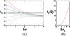 |
Fig. A.1 a) Profiles of the function f1(r) for several values of f1(0). b) Roots of f1(r), that is, values of f1(0) at which f1(r0) = 0. |
Figure A.1a shows profiles of f1 for several initial conditions, that is, f1(0) = 0, ± 1, ± 2, ± 3, by different colors and line types. For f1(0) > 0, the function has a root at r> 0, which means Br = 0 at it, so that the flux rope has a circular cross section there. The figure suggests that solutions have a common asymptotic behavior.
The value of f1(0) determines a location of a root. To construct a flux rope with an ideal toroidal shape with major and minor radii R0 and r0, respectively, and with a given b, we must fulfill the equation f1(r0) = 0. The function f1 implicitly depends on C1, which is related to f1(0), and an appropriate value of f1(0) can be found by a root-finding method. In fact, the function f1 depends on br, so that the same root at br0 yields the same value of f1(0); these values are shown in Fig. A.1b.
Appendix B: Magnetic helicity of the field given by the zero-order solution
The helicity is ![Mathematical equation: \appendix \setcounter{section}{2} \begin{eqnarray} H & = & \frac{B_0^2 \pi^2 R_t^2}{b^2 e_0} \left[\ln (4 e_0^4) \ln\left(\frac{e_2}{e_1} \frac{e_3}{e_4}\right) -\, \ln (e_1 e_2) \ln{\frac{e_2}{e_1}} \right. \nonumber \\[1mm] && - \, \ln (e_3 e_4) \ln{\frac{e_3}{e_4}} +4 \ln (e_0+b R_t) \ln (1+b^2 r_t^2) \nonumber \\[1mm] && \left. +\, 2 \mathrm{Li}_2{\frac{e_1}{2 e_0^2}}-2 \mathrm{Li}_2{\frac{e_2} {2 e_0^2}}-2 \mathrm{Li}_2{\frac{e_3}{2 e_0^2}}+2 \mathrm{Li}_2{\frac{e_4} {2 e_0^2}} \right], \label{H0} \end{eqnarray}](/articles/aa/full_html/2017/12/aa31412-17/aa31412-17-eq279.png) (B.1)where auxiliary variables are
(B.1)where auxiliary variables are 
 The helicity per unit length in the limit of high aspect ratios yields
  (B.7)which coincides with Eq. (60) and with the relative helicity per unit length for the cylindrical uniform-twist flux rope (Gold-Hoyle tube).
All Tables
All Figures
|
Fig. 1 Magnetic cloud of April 22, 2001. Observations (5-min averages) are plotted by the red lines, B, Bx, By, and Bz are the magnetic field magnitude and the field components in the GSE coordinates, V, N, and T are the solar wind velocity, proton number density, and proton temperature, respectively. Estimated cloud boundaries are drawn by the blue vertical lines. The thick green lines are fits by cylindrical models, namely a) the (spatially) constant-α force-free field (the Lundquist solution) with expansion, and b) (spatially) uniform-twist field (the Gold-Hoyle tube) with expansion. |
| In the text | |
|
Fig. 2 Toroidal flux rope with a uniform-twist field. One magnetic field line is drawn in red. It closes in on itself, and this holds for all field lines. This behavior only occurs for specific values of twist, otherwise the field lines are ergodic. |
| In the text | |
|
Fig. 3 a) Magnetic field magnitude distribution and b) distribution of angles δ between the field vectors and current for a toroidal flux rope with aspect ratio R0/r0 = 5, uniform-twist field, and unit-less twist br0 = 1.5. Lines are cross sections of magnetic field surfaces on which magnetic field lines lie. The thick line (circle) is the flux rope boundary. The magnetic field magnitude B is scaled by its maximum value Bmax inside the flux rope. The angle δ is zero for an exact force-free solution. |
| In the text | |
|
Fig. 4 Magnetic field profiles along the x axis for several flux ropes with R0/r0 = 5. Comparison of the MT solution (black lines) to the zero-order solution with several values of br0. The green lines are for br0 = 1, the blue lines for br0 = 2, and the red lines for br0 = 3. |
| In the text | |
|
Fig. 5 Magnetic field profiles for four flux ropes and along three different directions are shown in the middle part. Comparison of the MT solution (in black) to the zero- (in green) and first- (in red) order solutions and the uniform-twist solution (in blue). All flux ropes have circular cross sections with radius r0, R0/r0 = 5, and br0 = 1.5. Trajectories along which the profiles are displayed are shown by the thick arrows in the top sketches of the flux ropes. Panel a displays the profiles along the x-axis, panel b along the line parallel to the y-axis and crossing the x-axis at the point [R0−r0/ 2,0,0], and panel c along the line parallel to the z-axis and crossing the x-axis at the point [R0,0,0]. The bottom part shows hodograms of the magnetic field vectors along the displayed trajectories. The color coding of the lines is the same as in the middle part. The arrows show directions of the hodograms and also indicate the entry into the toroid (blue) and the exit (green). |
| In the text | |
|
Fig. 6 Magnetic field magnitude distribution (a, c) and distribution of angles δ between the field vectors and current (b, d) for a toroidal flux rope with aspect ratio R0/r0 = 5 given by the zero-order solution in the top panels (a, b), and by the first-order solution in the bottom panels (c, d). The lines are cross sections of magnetic field surfaces on which magnetic field lines lie. The thick line (circle) is the flux rope boundary. It is br0 = 1.5. |
| In the text | |
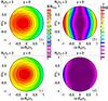 |
Fig. 7 Same as Fig. 6, but for an aspect ratio R0/r0 = 3. |
| In the text | |
|
Fig. 8 Twist |
| In the text | |
|
Fig. 9 Magnetic cloud of March 19–22, 2001. The format of the figure is the same as Fig. 1. The thick green lines are fits by toroidal models, namely a) the MT field with expansion, and b) the zero-order solution with expansion. |
| In the text | |
|
Fig. 10 Trajectory of a spacecraft (red arrows) through the model of the expanding toroidal flux rope, corresponding to the fit from Fig. 9b. The trajectory is shown in the intrinsic Cartesian system x, y, and z of the toroid, Eqs. (19)–(21) (the coordinates are different from the GSE coordinates), in projection to the a) yz-plane, b) xz-plane, and d)xy-plane; panel c displays the trajectory in a cross section of the toroid, where coordinates r and θ serve as polar coordinates. The blue lines are the boundaries of the toroid at the spacecraft entry, the green lines are the boundaries at the exit. According to the model assumptions, the minor radius of the toroid increases during expansion, while the major radius remains constant. |
| In the text | |
|
Fig. 11 Δ as a function of the aspect ratio for four magnetic field solutions: the uniform-twist field (ut, magenta), the zero-order solution (0-o, blue), the first-order solution (1-o, red), and the MT field (MT, green). The values of Δ are approximately one half of the ΔB values because the values of ΔV are small, see Eq. (61). |
| In the text | |
|
Fig. A.1 a) Profiles of the function f1(r) for several values of f1(0). b) Roots of f1(r), that is, values of f1(0) at which f1(r0) = 0. |
| In the text | |
Current usage metrics show cumulative count of Article Views (full-text article views including HTML views, PDF and ePub downloads, according to the available data) and Abstracts Views on Vision4Press platform.
Data correspond to usage on the plateform after 2015. The current usage metrics is available 48-96 hours after online publication and is updated daily on week days.
Initial download of the metrics may take a while.