Testing stellar evolution models with detached eclipsing binaries

J. Higl; A. Weiss

doi:10.1051/0004-6361/201731008

Home

All issues

Volume 608 (December 2017)

A&A, 608 (2017) A62

Full HTML

Free Access

Issue		A&A Volume 608, December 2017


Article Number		A62
Number of page(s)		15
Section		Stellar structure and evolution
DOI		https://doi.org/10.1051/0004-6361/201731008
Published online		07 December 2017

A&A 608, A62 (2017)

Testing stellar evolution models with detached eclipsing binaries

J. Higl¹^,2 and A. Weiss¹

¹ Max-Planck-Institut für Astrophysik, Karl-Schwarzschild-Str. 1, 85748 Garching, Germany
e-mail: higljoha@mpa-garching.mpg.de
² Technische Universität München, Physik Department, James Franck Str. 1, 85748 Garching, Germany

Received: 19 April 2017
Accepted: 7 September 2017

Abstract

Stellar evolution codes, as all other numerical tools, need to be verified. One of the standard stellar objects that allow stringent tests of stellar evolution theory and models, are detached eclipsing binaries. We have used 19 such objects to test our stellar evolution code, in order to see whether standard methods and assumptions suffice to reproduce the observed global properties. In this paper we concentrate on three effects that contain a specific uncertainty: atomic diffusion as used for standard solar model calculations, overshooting from convective regions, and a simple model for the effect of stellar spots on stellar radius, which is one of the possible solutions for the radius problem of M dwarfs. We find that in general old systems need diffusion to allow for, or at least improve, an acceptable fit, and that systems with convective cores indeed need overshooting. Only one system (AI Phe) requires the absence of it for a successful fit. To match stellar radii for very low-mass stars, the spot model proved to be an effective approach, but depending on model details, requires a high percentage of the surface being covered by spots. We briefly discuss improvements needed to further reduce the freedom in modelling and to allow an even more restrictive test by using these objects.

Key words: stars: evolution / stars: interiors / binaries: eclipsing

© ESO, 2017

1. Introduction

Many branches of astrophysics rely on accurate stellar models. Prime examples are the population synthesis of galaxies, the chemical evolution of stellar systems, and the rapidly advancing field of galactic archeology, which profits tremendously from progress in spectroscopy, asteroseismology, and astrometry. Therefore, the need for accurate stellar models is increasing and well-tested models are urgently needed. There are no test cases for stellar evolution that have analytical solutions except for simplified cases that ignore the complexity of constitutional physics; therefore one has to resort to observed objects. The most prominent object is the Sun, in which case we not only have the most precise measurements of global quantities (mass, radius, and luminosity), but also a determination of its age and composition. Even in view of the remaining uncertainty about the exact value of the latter (Asplund et al. 2009; Caffau et al. 2011; Villante et al. 2014), it is already sufficiently precise in the context of general stellar evolution. Finally, helioseismology has provided additional information about the internal structure of the Sun, which makes it an even more stringent test case. Therefore, it is well suited to determine additional free parameters that are not available from other sources, namely the mixing-length parameter α_MLT, present solar helium content, and initial composition.

The weakness of the solar test case is that it is restricted in terms of mass, composition, and evolutionary phase. Some physical aspects, such as additional mixing processes or rapid rotation, cannot therefore be tested, and one has to look for other objects. While asteroseismology might return a variety of objects with well-determined properties in the future, in this paper we concentrate on detached double-lined eclipsing binary systems (DDLEBs), which are the best-suited objects for stellar model verification after the Sun. Analyses of light curves and spectra of members of DDLEBs allow a very precise determination of the masses and radii of both components. Stellar mass and chemical composition, usually given as [Fe/H], form the two fundamental parameters that define the evolution of a non-rotating, non-interacting star. Under the assumption that both system members were born at the same time and from the same molecular cloud, the test for the theoretical model consists primarily in the requirement that both components reach the observed radii at the same age.

This method of testing stellar evolution models has a long tradition. A classical reference is the paper by Schröder et al. (1997), who determined the necessity or amount of core overshooting with ζ Aurigae systems. These systems contain a main-sequence secondary and a red giant primary in the phase of core helium burning, but are relatively rare because of the fast evolutionary speed of the primary. The authors found that their implementation of overshooting results in satisfactory matches of the data for an efficient overshooting of ~ 0.24···0.36 H_P (pressure scale heights), with a tendency towards increasing overshooting from the convective core with mass, ranging from about 3 to 6 M_⊙.

In a second paper, Pols et al. (1997) extended their tests to a sample of 49 binary systems, covering the full mass range from low-mass to massive stars, with parameters taken from Andersen (1991). In contrast to their first work they found no significant need for overshooting except for in the three systems AI Hya, WX Cep, and TZ For; all of these systems had components beyond the main sequence and in the mass range of 2–3 M_⊙. Nine systems could not be fitted at all.

Young et al. (2001) used a similar selection of objects from Andersen (1991) to test their stellar evolution code with models without overshooting. In summary they found acceptable fits in most cases, but they also identified a potential need for overshooting that increased with stellar mass and for stars of lower mass with a small convective core. Similarly, Meng & Zhang (2014) used four detached eclipsing binaries in the lower intermediate-mass range to calibrate the free parameter of their own treatment of convective overshooting, and found agreement with the value determined from main-sequence considerations (Zhang 2013).

After the update on binary system parameters by Torres et al. (2010), a renaissance of this basic test became possible. Stancliffe et al. (2015) used 11 of the listed systems plus 1 additional system for a new calibration of their overshoot treatment. The selected systems were those with components in advanced evolutionary stages. The models kept metallicity as an additional free parameter, not using spectroscopically determined abundances, for the simple reason that accurate abundances have simply not been available. This was also the case in most of the above-mentioned work. In all cases moderate overshooting, without a clear trend with stellar mass, was necessary for a good match.

Most recently, Valle et al. (2016) investigated by how much such calibrations of the amount of overshooting – or, more generally, the amount of extra mixing outside the Schwarzschild convective core boundary – depend on the uncertainties of the observed quantities. They concentrated on main-sequence stars and found that overshooting is poorly constrained, mainly due to the lack of a sufficient number of accurate observables. This is in agreement with the result of earlier work (see Pols et al. 1997; Young et al. 2001), which found, in general, that the preferred overshooting description provides satisfying matches, but did not necessarily exclude the non-overshooting hypothesis.

In this paper we use 19 DDLEB systems taken from different sources in the literature. We selected objects with very accurate mass and radius determinations and with published metallicities to constrain our models as much as possible. We modeled these systems using our own stellar evolution code Garstec (Weiss & Schlattl 2008). We restricted the variety of systems to such objects for which the components are either low-mass, older main-sequence stars, or stars with a convective core. The latter are useful for the standard overshooting test described above, but the former were chosen because we additionally aim at investigating how much atomic diffusion (sedimentation of heavier elements), which we know is taking place in the Sun, also affects the evolution of low-mass stars in general. For both physical effects, neither the occurrence nor their extent or strength is well known from first principles. Our objects also span a range of metallicities to widen the baseline for any composition-dependent effects.

In addition, we chose DDLEBs containing very low-mass stars, for which it is known that real stars have larger radii than simple models predict (see e.g. Kraus et al. 2011; Feiden & Chaboyer 2012). We find the same problem and show that it can be solved by adding a model for stellar spots to the models.

Our paper is organized as follows: in the next section we introduce the objects we are going to model, followed by a short description of the stellar evolution code and the fitting procedure (Sect. 3). The results of Sect. 4 are discussed in Sect. 5. The conclusion in the final section completes the paper.

2. Observational data

We selected 19 DDLEB systems with precisely determined masses and radii from the literature (Tables 1–3). Most of the stars in this study have relative mass and radius errors that are smaller than 2%, which restricts the input parameters of stellar models significantly. A collection of such systems can be found in Torres et al. (2010) and the online database DEBCat¹ described in Southworth (2015). In 11 of the selected systems both stars even have relative mass errors below 1%. Six of these systems also have relative radius errors that are smaller than the per cent level. Additionally there are three other systems with radius errors <1% and mass errors <2%. The mass error only exceeds 3% in 1 system and the radius errors are larger than 3% in 2 systems. The system with the least constraint input parameters is the ζ-Aurigae system V2291 Oph with mass and radius errors of 3.8 and 7%, respectively.

For any meaningful modelling, the surface composition of the stars is essential, even if it might not necessarily reflect the initial stellar composition. We therefore selected only systems where the surface iron abundance [Fe/H] has been determined. This restriction significantly different from comparable work (e.g. Schröder et al. 1997; Meng & Zhang 2014; Young et al. 2001; Stancliffe et al. 2015; Claret & Torres 2016), where metallicity (being sometimes not available for all objects) was often varied to find the best fit. For most of our systems [Fe/H] was determined by a spectroscopic analysis of the system itself (indicated by [s] in the [Fe/H] column of Tables 1–3). In the tables, we list either the metallicity of the system or of the primary. If a system is a member of a cluster and no detailed spectroscopic observation of the system itself is available, we use the [Fe/H] value of the cluster (indicated by [c]). [Fe/H] for MU Cas was determined from photospheric indices (indicated by [p]). The surface metallicity of Cepheids in the Large Magellanic Cloud has been determined by Romaniello et al. (2008). We use this value for the system OGLE-LMC-CEP-0227 (from now on CEP-0227; indicated by [lmc]).

A low mass ratio q = M_B/M_A increases the sensitivity of testing model parameters because the tests are then performed over a wider range of masses or even in different evolutionary phases with otherwise similar conditions. An example would be the amount of overshooting for a pair of stars with a small and large convective core (see Sect. 3.2 and the treatment in Pietrinferni et al. 2004). We therefore prefer systems with a lower mass quotient over systems with similar masses. In fact, 11 of our systems have q < 0.9.

The observational data of the systems are given in Tables 1–3. We denoted the more evolved star (= the more massive star) as star “A”, which differs from the convention in some observational papers.

3. Stellar models and procedure

3.1. Canonical model assumptions

Under the realistic assumption that components of DDLEB systems have been evolving without interaction, one computes single-star models for both, using the observational values for mass and composition. We performed all computations with our own stellar evolution code Garstec (Weiss & Schlattl 2008), initially under canonical (standard) physical assumptions, which have been modified if a simultaneous fit for both components could not be achieved. Standard models use a solar calibrated α_MLT = 1.74 (see Weiss & Schlattl 2008) and start from the pre-main sequence. The solar calibration is always done for a Standard Solar Model, implying that atomic diffusion is included, irrespective of whether we also take it into account in the model calculations. The solar composition was assumed to be that of Grevesse & Sauval (1998).

Our models use the equation of state (EOS) tables by the OPAL group (Rogers & Nayfonov 2002). They do not extend to the low-temperature, high-pressure regime of fully convective, very low-mass stars. For these types of stars we used the unpublished SCOPE tables, which are described in Weiss (1999). These EOS tables are a combination of the OPAL, Saumon-Chabrier (Saumon et al. 1995), and Eggleton-Faulkner-Flannery (EFF) EOS (Pols et al. 1995).

Almost all computations were performed with OPAL opacity tables (Iglesias & Rogers 1996) with the internal solar metallicity distribution described in Seaton et al. (1994), which is virtually identical to the composition of Grevesse & Noels (1993). At low temperatures the tables are extended by the Wichita State Alexander and Ferguson molecular opacity tables (Ferguson et al. 2005). In some cases we also constructed models with a recalculated set of opacity tables with the metallicity distribution of Grevesse & Sauval (1998). These models are marked with an asterisk in the tables. We found that the conclusions made in this study do not depend on the internal metallicity distribution used in the opacity tables. Nuclear reaction rates were taken from the NACRE collection (Angulo et al. 1999), with the exception of the crucial bottleneck reaction of the CNO cycle, ¹⁴N(p,γ)¹⁵O, for which we used the newer rate by Marta et al. (2008).

Deviations from these canonical physics assumptions are discussed below and criteria for the observed objects for which they had been applied are specified.

3.2. Additional physical options

Depending on the structure of the star, we also computed alternative models including additional physical effects not included in the standard models.

Convective overshooting.

Convective overshooting is a physical process that certainly takes place at all convective boundaries; the efficiency of this model, however, is unknown. Therefore it is implemented in stellar evolution codes in one way or another as a parametrized, additional mixing process. Also the resulting temperature gradient in the overshooting region is subject to some assumption. In Garstec overshooting is implemented as a diffusive process according to the description of Freytag et al. (1996). The diffusion constant as a function of the distance z from the formal Schwarzschild border is given as 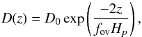$D (z) = D_{0} \exp (\frac{- 2 z}{f_{ov} H_{p}}),$ $\begin{equation} \label{oveq} D(z)=D_0\exp\left(\frac{-2z}{f_{\rm ov} H_p}\right) , \end{equation}$ (1)where D₀ = 1/3v₀·H_p is a scale for the diffusive speed. While H_p is taken at the formal Schwarzschild border, the convective velocity v₀ is evaluated half a pressure scale height interior to that border, as in mixing-length theory v₀ vanishes at the border by definition. The free parameter, f_ov, is f_ov = 0.02. This value corresponds to an overshooting of about 0.2 H_p in the classical local description and has been chosen since it allows an efficient modelling of the colour-magnitude diagram of open clusters (Magic 2010; Magic et al. 2010), and agrees, in addition, with the result by Claret & Torres (2016) for stars above 2 M_⊙.

We used the same parameter for all convective boundaries. This is certainly only one possible choice, but we considered a restriction, say, to only hydrogen-burning cores, as arbitrary as well, and an individual “calibration” for any given convective boundary is still beyond current possibilities (see Miller Bertolami 2016, for a discussion, and an attempt to do so).

Our study also includes models with very small convective cores. As H_p diverges towards the centre, this would lead to an unrealistically large overshooting region both in the classical and in the diffusive description. To avoid this problem several authors have used an overshooting parameter that depends on the main-sequence mass (e.g. Pietrinferni et al. 2004). In our case, the same effect – but now valid for all thin convective layers – is achieved by implementing a geometrical cut-off. We replaced H_p in the argument of the exponential of Eq. (1) by $\begin{matrix} ˜ \\ H_{p} \end{matrix} = H_{p} \cdot \min [1, {(\frac{Δ R_{CZ}}{H_{p}})}^{2}] \cdot$ $\begin{equation} \tilde{H}_p = H_p \cdot \mathrm{min}\left[1,\left(\frac{\Delta R_{\rm CZ}}{H_p}\right)^2\right] \cdot \end{equation}$ (2)This ensures that the size of the overshooting region is limited to a fraction of the convective zone (thickness ΔR_CZ). Its form was chosen as it also allows a successful representation of the turn-off morphology of old open clusters, and the disappearance of the transient convective core appearing during the solar pre-MS evolution (see Schlattl & Weiss 1999).

Atomic diffusion.

Although atomic diffusion is a basic physical effect, it is unclear to what extent it occurs in stars. Because of the extremely low diffusive velocities (of the order of 10^-10 cm/s in the Sun) and timescales in main-sequence stars, which are comparable to or even longer than nuclear timescales, any counteracting mixing process or structural changes may inhibit it. This was demonstrated by Vauclair & Charbonnel (1995) in the case of a moderate stellar wind opposing the effect of gravitational settling in solar-like stars. While in the case of the Sun, the straightforward inclusion of atomic diffusion following the description by Thoul et al. (1994) or using the diffusion coefficients by Paquette et al. (1986) is a necessary requirement for the best agreement with helioseismology (Bahcall & Pinsonneault 1992), it is unclear whether such inclusion of atomic diffusion works with the same efficiency in other stars. While Gratton et al. (2001) claimed the lack of any clear sign of diffusion in the globular clusters NGC 6397 and NGC 6752, Korn et al. (2007) reported evidence for settling in the former cluster. In their models, however, they had to include “turbulent diffusion” to reduce the depletion of heavy elements from the photosphere of cluster dwarfs to the level they identified from their spectral analysis. Further arguments for the effectiveness of gravitational settling comes from the effect on the colour or effective temperature of stars. Jofré & Weiss (2011) demonstrated that the turn-off colours of metal-poor stars in the SDSS samples can be reproduced at an age that is consistent with that of the Galaxy only if unrestricted diffusion is allowed in stellar models. Evidently, all these arguments relate to the effect of diffusion in the (sub-)photospheric layers of stars. However, an equally important effect is that diffusive settling shortens the main-sequence lifetime by removing hydrogen from the burning core. Chaboyer et al. (2001) suggested a separate treatment of both regions that inhibits diffusion artificially beneath the surface, but allows for unrestricted diffusion in the central regions. This needs further investigation, and therefore we investigated the effect of diffusion in our objects. To avoid the introduction of additional free parameters we always applied diffusion in the same way as in solar models, thereby obtaining the most extreme effect.

As described in Weiss & Schlattl (2008) we included diffusion in our models using the description of Thoul et al. (1994). Besides $1 H$ $\hbox{${}^1\mathrm{H}$}$ and $4 He$ $\hbox{${}^{4}\mathrm{He}$}$ , we also followed the distribution of several heavier elements and their isotopes ( $12 C, 13 C, 14 N, 15 N, 16 O, 17 O, 20 Ne, 24 Mg, 28 Si, 56 Fe$ $\hbox{${}^{12}\mathrm{C}, {}^{13}\mathrm{C}, {}^{14}\mathrm{N}, {}^{15}\mathrm{N}, {}^{16}\mathrm{O}, {}^{17}\mathrm{O}, {}^{20}\mathrm{Ne}, {}^{24}\mathrm{Mg}, {}^{28}\mathrm{Si}, {}^{56}\mathrm{Fe}$}$ ). Since diffusion reduces the surface abundances of all elements heavier than hydrogen over time, the initial abundances are an additional free parameter to be set in such a way as to match the present and observed metallicity.

Stellar spot model.

Several systems discussed below (Sect. 4.1) contain very low-mass stars. For such cool dwarfs it is well established that canonical stellar models have too small radii compared to observed values (see e.g. Torres et al. 2010; Feiden & Chaboyer 2014, and references therein). This failure of stellar models is usually ascribed to a lack of physics considered, in particular in connection with magnetic activity. In the present paper, we took this into account by applying a simple model for stellar spots (Spruit & Weiss 1986).

Spots block part of the convective flow to the surface, which reduces the surface temperature. As a consequence the star has to expand to radiate its energy. Following Spruit & Weiss (1986), we mimic the effect of spots in our models by introducing an effective spot coverage f_e, which depends on the fractional areas of the umbrae (f_u) and penumbrae (f_p) with temperatures T_u and T_p, respectively. The value f_e is defined as $\begin{matrix} f_{e} & = & [b a^{2} + c (1 - a^{2})] f \\ f & = & f_{u} + f_{p} = 1 - f_{0} \\ a^{2} & = & \frac{f_{u}}{(f_{u} + f_{p})} \\ b & = & 1 - \frac{T_{u}^{4}}{T_{0}^{4}} \\ c & = & 1 - \frac{T_{p}^{4}}{T_{0}^{4}}, \end{matrix}$ $\begin{eqnarray} f_{\rm e} &=& [ba^2 + c(1-a^2)]f \\ \label{e:spot} f &=& f_{\rm u} + f_{\rm p} = 1 - f_0 \\ a^2 &=& \frac{f_{\rm u}}{(f_{\rm u}+f_{\rm p})} \\ b &=& 1- \frac{T_{\rm u}^4}{T_0^4} \\ c &=& 1- \frac{T_{\rm p}^4}{T_0^4} , \end{eqnarray}$ where T₀ is the temperature of the unspotted area f₀. The Stefan-Boltzmann law then becomes $L = 4 πσ R^{2} T_{0}^{4} (1 - f_{e}) .$ $\begin{equation} L = 4 \pi \sigma R^2 T_0^4 (1- f_{\rm e}) . \end{equation}$ (8)With this formulation we are able to increase the size of a stellar model, depending on the parameters of the spot model. In order to make the effective temperatures of the models comparable to the observations, we have to account for the spot coverage as well because T_eff of the models represent the unspotted parts of the surface, while observations represent an average over spotted and unspotted areas. Hence our new $\begin{matrix} ˜ \\ T_{eff} \end{matrix}$ $\hbox{$\tilde{T}_\mathrm{eff}$}$ is $\begin{matrix} ˜ \\ T_{eff} \end{matrix} = 4 \sqrt{T_{eff}^{4} (1 - f_{e})} .$ $\begin{equation} \tilde{T}_{\mathrm{eff}}=\sqrt[4]{T_\mathrm{eff}^4(1-f_{\rm e})} . \label{e:ttilde} \end{equation}$ (9)It is obvious that such a model, which allows us to tune the stellar radius to the desired value, reduces the predictive power of our models. Nevertheless, it allows us to check for consistency with other observables and whether the model itself is reasonable (for example, by using the same parameters a, b, and c for all objects).

3.3. Procedure

For each object we computed a grid of at least 3 × 3 models for the central values of the given mass and metallicity and for the upper and lower values of the error range. We interpret these errors as 1σ errors. The initial composition was determined in the following way. The total metallicity Z was obtained from the given [Fe/H]-value, assuming the solar-like heavy element distribution of Grevesse & Sauval (1998). With two exceptions there are no objects in our sample that have any indication of an α-element enhancement or any other deviation from this assumption. The helium content was calculated assuming a helium enrichment law of Y = 0.248 + 2Z, where 0.248 is the primordial helium content (Peimbert et al. 2007; Cyburt et al. 2008) and Z the metallicity according to the central value of the [Fe/H] range. This value of the relative mass fraction of helium was kept constant independent of the uncertainty range of [Fe/H]. For models including diffusion these starting values had to be adjusted accordingly to match observed values at the present stellar age. If not mentioned otherwise, we used the 1σ mass range and the central values for metallicity for the resulting fits presented.

Table 1

Fundamental parameters of lower mass main-sequence systems (Sect. 4.1) ordered by increasing mass of the primary star A.

The models for both components of each system were then evolved until they each reached the observed radius. Since the basic assumption is that both components are coeval, a successful match necessarily has to return the same age for both stars when their respective radii are matched. As a by-product this would also be the system age. We consider a system to be fitted successfully if the radius of each model is within the given 1σ error range of the mean observed value.

In this case we additionally compared the more indirectly determined temperatures and luminosities of the objects with those predicted by our models in the usual Hertzsprung-Russell diagram (HRD). In most cases the luminosity was determined in the original paper by applying the Stefan-Boltzmann law, using the geometrically determined stellar radius and the independently determined T_eff. The source for the latter quantity varies between objects and can be due to earlier literature values, photometric estimates, or from the same spectroscopic analysis that also returned the metallicity. The uncertainty of the luminosity correlates with that of T_eff and R and therefore the error box in the HRD is skewed.

A more direct method for an additional check of our models is the comparison of T_eff and L ratios of the two binary components. These ratios can be determined directly from the light curves of DDLEBs. In an ideal case, with circular orbits and spherical stars, the temperature ratio can be estimated from the measured fluxes during and outside the eclipses. The measured flux outside of eclipse, at distance d, is B₀ = (L_A + L_B)/(4πd²). If star A is the larger one, the flux during the primary eclipse B_p and during the secondary eclipse B_s is given as 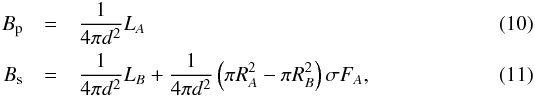$\begin{matrix} B_{p} & = & \frac{1}{4 π d^{2}} L_{A} \\ B_{s} & = & \frac{1}{4 π d^{2}} L_{B} + \frac{1}{4 π d^{2}} (π R_{A}^{2} - π {R_{B}^{2}}^{)} σ F_{A}, \end{matrix}$ $\begin{eqnarray} B_{\rm p} &=&\frac{1}{4\pi d^2} L_A \\ B_{\rm s} &=&\frac{1}{4\pi d^2} L_B + \frac{1}{4\pi d^2} \left(\pi R_A^2 - \pi R_B^2\right)\sigma F_A , \end{eqnarray}$ where we used the Stefan-Boltzmann law L = 4πR²F and $F = σ T_{eff}^{4}$ $\hbox{$F = \sigma T_\mathrm{eff}^4$}$ . The depth of an eclipse is the difference of fluxes during and outside of eclipse. Taking the ratio of the depth of the two eclipses, we immediately get the temperature ratio of the system 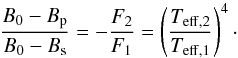$\frac{B_{0} - B_{p}}{B_{0} - B_{s}} = - \frac{F_{2}}{F_{1}} = {(\frac{T_{eff, 2}}{T_{eff, 1}})}^{4} \cdot$ $\begin{equation} \frac{B_0-B_{\rm p}}{B_0-B_{\rm s}}=-\frac{F_2}{F_1}=\left(\frac{T_\mathrm{eff,2}}{T_\mathrm {eff,1}}\right)^4 \cdot \end{equation}$ (12)Using this temperature ratio in combination with the measured ratio of radii and the Stefan-Boltzmann law we can also get the ratio of luminosities. A similar method was used in Claret (2007). This comparison has the biggest significance when at least one of the stars is in a fast evolutionary phase beyond the main sequence.

A perfect solution would be a solution that passes all three tests mentioned. In reality this is very rarely the case. Since in particular the absolute T_eff values have to be taken with care, we assign the highest weight to fits in the R(t) diagram. An additional match within the error boxes in the T_eff,p/T_eff,s vs. L_p/L_s diagram is taken as further confirmation, while we consider a mismatch in the HRD only as a potential problem because we think that the absolute values of T_eff and L are in many cases questionable, and certainly do not reach the precision of the mass and radius determinations.

Table 2

As Table 1, but for more massive main-sequence systems with components that have a convective core.

4. Results

We divided our results into three categories according to the evolutionary state and mass of the primary star A. Objects with both stars on the MS are separated into two categories below and above 1.2 M_⊙ (see Tables 1 and 2 for a list of objects). This is approximately the mass where stars change from a radiative to a convective core on the MS. While overshooting can be ignored for the lower mass category, it plays an important role in the determination of the age for more massive stars.

The effect of overshooting is even more noticeable for systems that have at least one component evolved beyond the MS, where the increased core has a larger luminosity. The extended convective envelopes beyond the MS are also affected by overshooting, which can change the morphology of the evolution significantly. We therefore collected more evolved systems in a separate category (see Table 3).

4.1. Main-sequence systems: M < 1.1 M_⊙

Fig. 1

Model evolution of V565 Lyr. Horizontal areas with dashed central lines represent the observed error ranges. The solid line represents the evolution with the mean observed mass and the areas around it represent the 1σ mass range (see Table 1). The two panels show the radius evolution of the primary (top) and secondary (bottom) for V565 Lyr with [Fe/H] _i = 0.40, Y_i = 0.32. The models include diffusion. Within the errors a common age of 7.08 ± 0.15 Gyr is found (vertical lines).

Fig. 2

As Fig. 1, but for V568 Lyr. The common age is 6.57 ± 0.14 Gyr.

V565 Lyr and V568 Lyr.

Both systems are members of the metal-rich open cluster NGC 6791 and consist of a solar-like primary that approaches the end of the MS and a solar-like companion still on the MS. Fundamental parameters for both systems are given in Brogaard et al. (2011), but for V568 Lyr we used the updated values by Yakut et al. (2015). Observations by Brogaard et al. (2011) show a mean difference of ±0.05 dex in [Fe/H] between the primaries, which is also the upper limit for the observed colour spread in the cluster, which results from the metallicity difference (Brogaard et al. 2012). Our standard models with the observed initial metallicities (Table 1), however, fail to give a common age for any of the two systems and tend to have temperatures that are too high.

In general, all cluster members are expected to have the same initial composition. Results for the metallicity of cluster giants range between [Fe/H] = 0.32 (Worthey & Jowett 2003) and 0.47 (Gratton et al. 2006; Carretta et al. 2007) with intermediate values close to [Fe/H] = 0.4 by Peterson & Green (1998) and Carraro et al. (2006).

Assuming that the cluster composition is represented by the surface composition of giants, we computed a set of models including diffusion with a unique initial composition of [Fe/H] = 0.4 ± 0.1, Y = 0.322 (results are shown in Figs. 1 and 2). With these models we found system ages of 7.08 ± 0.15 Gyr and 6.57 ± 0.14 Gyr for V565 Lyr and V568 Lyr, respectively. This is in excellent agreement with the ≈7.0 Gyr as given in Brogaard et al. (2011) for the DDLEBs, and in rough agreement with a cluster age of 8.3 ± 1.4 Gyr estimated additionally from the CMD (Brogaard et al. 2012). We also match the current surface metallicities of the primaries for both systems and that of the secondary of V565 Lyr ([Fe/H] = 0.22 ± 0.1; Brogaard et al. 2011). For the secondary of V568 Lyr there is no separate abundance measurement.

The observed luminosity and temperature ratios were matched over the whole MS evolution. The age difference of 510 Myr could be explained by a prolonged star formation in NGC 6791, which may have lasted between 0.3 Gyr (Brogaard et al. 2012) and 1 Gyr (Twarog et al. 2011).

NGC 6791 also hosts a third EB with determined masses and radii. Brogaard et al. (2011) give masses for V633 Lyr (1.0588 ± 0.0091 M_⊙ and 0.8003 ± 0.0062 M_⊙), which are very similar to V568 Lyr. The uncertainty in the radius determination (1.341 ± 0.081 R_⊙ and 0.90 ± 0.18 R_⊙) is too large to constrain the models further. We match the radii of V633 Lyr between 6 and 8 Gyr and also reproduce the observed metallicity.

M55 V54.

The globular cluster M55 has a metallicity, determined from giants, of [Fe/H] =−1.83 (Kaluzny et al. 2014), which makes M55 V54 the system with the lowest metallicity in this study. The cluster is also α-enhanced. We took this as the initial composition of our models, assuming [α/Fe] = + 0.4, and using consistent α-enhanced opacity tables. There are no abundance determinations available for V54 itself. To fit the system with an age lower than the cosmological age, diffusion needs to be included, as this accelerates the evolutionary speed. At the given radii of 1.01 and 0.53 R_⊙ both components give a lower limit on the age of 13.2 Gyr, in perfect agreement with the turn-off age of M55 determined by Dotter et al. (2010) and Kaluzny et al. (2014).

V636 Cen.

The primary of V636 Cen is a MS star of 1 M_⊙ at a subsolar metallicity of [Fe/H] =−0.2. Modelling this primary together with its 0.2 M_⊙ less massive companion, it became evident that it is not possible to fit this system with standard physics. Models of the secondary are too small and too hot compared to the observational estimates, indicating the known problem of model radii for very low-mass stars. Clausen et al. (2009) mentioned that the secondary shows signs of spot activity, and for these reasons we applied our simple spot model of Sect. 3.2.

With this formulation we were able to increase the size of the secondary such that it matches the observations at the same time as the primary (Fig. 3). It requires, however, an effective spot coverage of f_e = 0.33, which translates into an unrealistic coverage of 100% of solar-like spots (a = 0.4, b = 0.75, c = 0.25). Spruit & Weiss (1986) also point out that spots tend to lose their penumbrae in areas where the distance between spots gets comparable to their size. Under this assumption and an umbra with T_u = 0.7 T₀, both model sets with and without diffusion fit the observations with a coverage of 44%.

The modified effective temperatures $\begin{matrix} ˜ \\ T_{eff} \end{matrix}$ $\hbox{$\tilde{T}_\mathrm{eff}$}$ (Eq. (9)) also fit the observed temperature ratio, while the absolute T_eff of the secondary as given in Clausen et al. (2009) is still lower than our model value.

Kepler-16

is a planet hosting system at solar metallicity with a primary of 0.7 M_⊙. The secondary is a fully convective M dwarf of 0.2 M_⊙, which made it necessary to use the SCOPE EOS tables (Weiss 1999), described in Sect. 3.1, for this object. We also used these tables for the more massive primary, but verified that this does not lead to any difference in the MS evolution of component A, when compared to the use of the OPAL EOS.

Within the metallicity error we found an age of the primary between 0.5 and 3.0 Gyr for models without diffusion. The radius of the secondary on the other hand is 8% larger than predicted by the models. This difference can be overcome by assuming that at least 3% of the surface of the secondary is covered in solar-like spots. Because of the young age and fully convective secondary, we did not investigate the effects of diffusion in this system.

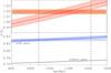Fig. 3

Evolution of V636 Cen models. Same as the top two panels of Fig. 1, but for V636 Cen with [Fe/H] =−0.20, Y = 0.27 and an effective spot coverage of f_e = 0.33. In the lower panel, the additional black line shows the radius evolution of the secondary, if no spots are assumed.

4.2. Main-sequence systems: M > 1.2 M_⊙

In this section we discuss those system that have both components still on the main sequence, but are massive enough that at least one of them has a convective core (for the system parameters, see Table 2). We place special emphasis on the question of whether convective core overshooting is needed or disfavoured.

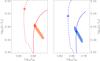Fig. 4

HRD of UX Men. Full lines show the evolutionary track of the models with diffusion and an initial metallicity of [Fe/H] _i = 0.2 and Y_i = 0.29. Dashed lines show tracks of standard models with the same mass, but without diffusion and a composition of [Fe/H] = 0.04, and Y = 0.28. All tracks are indicated at 2.1 Gyr. The red and blue shaded areas show the observational errors (as explained in Sect. 3.3) of primary (left panel) and secondary (right panel), respectively.

UX Men and KOI-3571.

Both stars of the solar metallicity system UX Men are relatively young MS stars and have about 1.2 M_⊙. Given the almost identical masses, both components should be very similar; thus for any assumption about the constitutive physics, such as the extent of overshooting, a solution for coeval target radii or the ratio of T_eff or L should be found, which is indeed the case. In this case we additionally used the position in the HRD as a fitting criterion. Standard models fit the observed radii, luminosity, and temperature ratios at an age of 2.2 ± 0.5 Gyr. The absolute temperatures of standard models, however, are higher than the observed values. Since the system is still at the beginning of its MS, overshooting is not expected to have a big impact. In fact the implemented overshooting results in an almost negligible 1% age increase. Andersen et al. (1989) measured [Fe/H] = 0.04 ± 0.1 for the whole system, but also provided separate [Fe/H] estimates for the primary and secondary of 0.00 ± 0.1 and 0.07 ± 0.1, respectively. This indicated difference may be a result of diffusive settling. While its effect on age can be ignored, diffusion requires a higher initial metallicity, which reduces the temperatures to the observed values (see Fig. 4). Both stars reach the target temperatures, radii, and surface metallicity at the same age. This would not be possible if the efficiency of our diffusion description were reduced.

The components of KOI-3571 have similar masses as those in UX Men (1.2 and 1.0 M_⊙), however the secondary has a radiative core. KOI-3571 is a member of the open cluster NGC 6819 with metallicity [Fe/H] =−0.02 ± 0.02 (Lee-Brown et al. 2015). It can also be fitted easily by standard, overshooting, and diffusion models, but the absolute temperatures can only be reproduced by including diffusion. We used an initial [Fe/H] of 0.13, at the upper end of the observed value of cluster red clump stars of [Fe/H] = 0.09 ± 0.03 by (Bragaglia et al. 2001). With this initial composition the primary matches the metallicity of MS stars at the time of the fit. The secondary, as a result of its more massive convective envelope, at that time still has a surface metallicity of ~ 0.07. The predicted metallicity difference between both components could be tested by detailed spectroscopic determinations. Both UX Men and KOI-3571 therefore do not offer any conclusions about core overshooting, but provide additional arguments for the full inclusion of diffusive settling.

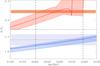Fig. 5

Models for BG Ind at [Fe/H] = −0.2; Y = 0.27, including overshooting. The panels are the same as in Fig. 1.

BG Ind

is important for this study because its primary is right at the end of the MS, where overshooting has the biggest effect. In this case only models including overshooting are able to give a common age for the system of 3.3 Gyr, also matching the observed temperature and luminosity ratios (see Fig. 5). Furthermore, standard models of the primary would be on the Hertzsprung gap, which is in disagreement with the observed luminosity. Rozyczka et al. (2011) obtained an age of only 2.65 ± 0.2 Gyr with the classical local description of overshooting in combination with a ramp function between 1.2 and 1.4 M_⊙. This may be an indication that our description of overshooting leads to a larger overshooting area in this mass range.

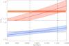Fig. 6

Same as in Fig. 1, but for KIC 9777062; the models include diffusion and overshooting. The composition is [Fe/H] _i = 0.04 and Y_i = 0.28.

KIC 9777062

is a member of the open cluster NGC 6811. Molenda-Żakowicz et al. (2014) determined the cluster metallicity ([Fe/H] = 0.04 ± 0.01; only internal errors) from giants. In an analysis by Sandquist et al. (2016) the masses of the two MS stars were determined to be 1.6 and 1.4 M_⊙; the spectral analysis of the primary revealed a high metal ([Fe/H] = 0.46) and low Ca ([Ca/H] =−0.80) abundance, which is a fact that could be an indication of the Am phenomenon. Since this is a surface effect it is most likely that the actual composition is not represented by these values. The secondary, in contrast, has [Fe/H] =−0.03 ± 0.13, which is consistent with the cluster metallicity. We used the cluster metallicity by Molenda-Żakowicz et al. (2014) for our models, but increased the error to 0.1 dex to account for systematic uncertainties and the larger uncertainty of the measurement of the binary system itself. Our best fit for this system uses the joint assumption of diffusion and overshooting; the system age, for [Fe/H]_i = 0.04, is 1.09 ± 0.07 Gyr (Fig. 6), which is in excellent agreement with the cluster age of 1.00 ± 0.05 Gyr, resulting from isochrone matching (Sandquist et al. 2016). If we omit either of these effects we are unable to find a solution with a common age agreeing with this value, in agreement with similar attempts by Sandquist et al. (2016). Our solution also reproduces temperature and luminosity ratios, but the absolute temperatures could be matched only when assuming the lower end of the metallicity range ([Fe/H] =−0.06). The resulting age would then be 1.18 Gyr.

Table 3

As Table 1, but for systems with components evolved past the main sequence.

MU Cas and V906 Sco.

These are two systems with intermediate-mass MS components and a mass ratio very close to 1. V906 Sco is a member of NGC 6475, which was suspected to have an overabundance in helium (Y = 0.33) at solar metallicity (Villanova et al. 2009). Modelling the 3.4 M_⊙ primary and its 3.3 M_⊙ companion, using this helium content, fails to reproduce the observed position in the HRD. Models using the helium enrichment law given in Sect. 3.3, on the other hand, match the given luminosity.

Regardless of this uncertainty in Y, overshooting as well as standard models give the observed radii at a common age and can also match the observed temperature and luminosity ratios. The standard models place the primary beyond the MS, while overshooting models place the primary right at the turn off, making them somewhat more likely as this is the longer lived phase.

In the case of MU Cas (4.6 and 4.5 M_⊙) even less can be said. The system has a supersolar metallicity of [Fe/H] = 0.22 from Strömgren photometry (Lacy et al. 2004). Since no error is given, we assumed one of ±0.2 dex. To model this system we had to use the upper (lower) end of the mass range for the primary (secondary). The system age results in 72 and 76 Myr for the standard and overshooting cases, respectively.

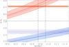Fig. 7

Models for V453 Cyg, with a metallicity of [Fe/H] = −0.04; Y = 0.27, and allowing for overshooting. The black lines in the top two panels indicate the alternative evolution with standard physics, but [Fe/H] = −0.24.

V453 Cyg.

In this case the conclusion about the need for overshooting depends on the metallicity of the system. Using the central value of [Fe/H] = −0.24, as in Table 2, we obtained a fit only for excluding it. The primary (14.4 M_⊙) is ending the MS phase or is even slightly beyond it; the secondary (11.1 M_⊙) is in it. Models including overshooting require an increase of metallicity to the upper edge ([Fe/H] = −0.04) to obtain a common age with both stars well on the MS (Fig. 7). The temperature ratio is fitted as well. We prefer the overshooting models over the standard models, because they are in the longer lived phase.

V380 Cyg.

This object has a metallicity of [Fe/H] = −0.40 including an overabundance of Mg and Si by about 0.4 dex, and of 0.2 dex in O (Tkachenko et al. 2014), possibly representing one of the interesting young objects with unusual composition found by Martig et al. (2015) and Chiappini et al. (2015). Both standard and overshooting, α-enhanced models fit the observed radii at an age of 16 and 18 Myr, respectively, and also reproduce temperature and luminosity ratios. However, they miss the absolute luminosity by a factor of two; this luminosity could be reproduced, if the overshooting parameter would be increased to f_ov = 0.06, which would, however, result in an age difference of 5 Myr between the two components. This could be an indication of either a mass-dependent amount of overshooting, or a hint towards a mixed core, increased by rotation-induced mixing, as Tkachenko et al. (2014) noted that the primary rotates at 32% of its critical velocity.

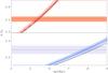Fig. 8

As Fig. 5, but for standard models of V578 Mon with a metallicity of [Fe/H] = −0.17; Y = 0.27. The additional black lines indicate models of the mean mass with overshooting.

V578 Mon.

The primary of V578 Mon is the most massive star of this study (14.5 M_⊙). As its 10.3 M_⊙ companion it is in the MS phase. In agreement with the result of Garcia et al. (2014) none of our models were able to give a common age for this system. With the subsolar metallicity [Fe/H] = −0.30 ± 0.13 by Pavlovski & Hensberge (2005), the secondary appears to be at least 30% older (see Fig. 8). Garcia et al. (2014) suggested an increased overshooting parameter in the primary to make it longer lived and therefore reduce the age difference between the two stars. However, since overshooting has a very small effect (see black lines in Fig. 8) and the secondary shows an even stronger increase, this is not a viable solution. On the other hand, increasing the metallicity seems to be a more promising approach. As a test, we assumed solar metallicity and neglected overshooting, finding the age difference to be reduced to 14%.

In this mass range, we found strong evidence in only two cases (BG Ind and KIC 9777062) and circumstantial evidence in some cases (e.g. V380 Cyg) for the need for overshooting. On the other hand, the standard models are only able to fit the system at the central value of the metallicity range for V453 Cyg. If we increase this value within the error range, overshooting models are possible again.

4.3. Evolved systems

AI Phe.

The masses of the components of AI Phe, for the parameters of this and the other systems in this section (see Table 3), are almost identical to those of UX Men, but the system is more evolved. Andersen et al. (1989) determined a slightly lower metallicity for the secondary ([Fe/H] = −0.17 ± 0.1) than for the primary ([Fe/H] = −0.13 ± 0.1), which is an indication of the effect of diffusion on the main sequence and the restoring effect of the first dredge-up on the RGB for the primary. We therefore assumed that its metallicity is very close to the initial value and included diffusion in our models, but we had to use a value of [Fe/H] = −0.04 at the upper limit of the 1σ range to match radii and present surface metallicities for both components. The [Fe/H] value given in Table 3 is the suggested combination of the two separate observations. The resulting system age is 4.68 Gyr, and the primary and secondary have [Fe/H] = −0.04 and [Fe/H] = −0.2, respectively, in agreement with the uncertainty range of Andersen et al. (1989, see Fig. 9). Including overshooting, on the other hand, results in a mismatch of age by 4%. This contradicts Pols et al. (1997), who found that overshooting and standard models fit equally well. Lastennet & Valls-Gabaud (2002) also were able to fit the system with overshooting models. They, however, had to reduce the metallicity of their models below the observed metallicity to achieve this.

V501 Her

is another system with stars that have a very small convective core, but in contrast to AI Phe it has a supersolar metallicity of 0.21. Since the given metallicity is only a rough estimate from a comparison of V501 Her and HR 3951 by Sandberg Lacy & Fekel (2014), we decided to choose a rather large uncertainty of ±0.2 dex. But even within this large metallicity range, standard models fit both radii at best with a 1% difference in age. In contrast, overshooting models give a common age, when a metallicity of [Fe/H] = 0.4 is assumed. In this case, they fit the HRD and temperature and luminosity ratios simultaneously. With an initial [Fe/H] of 0.6, models with diffusion also give a fit in the age-radius diagram, while the HRD is not matched. Since none of the physical effects can be ruled out, but require different initial metallicities, this system is an example that a more detailed abundance analysis of this system is needed to distinguish between different scenarios.

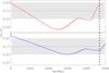Fig. 9

Evolution of [Fe/H] in AI Phe. The initial metallicity is assumed to be [Fe/H] _i = −0.04; Y_i = 0.27. The upper panel indicates the primary; the lower panel indicates the secondary component. The system age, indicated by the dashed line, is 4.681 ± 0.005 Gyr.

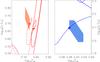Fig. 10

HRD of V2291 Oph models with [Fe/H] = 0.23; Y = 0.33 including overshooting and for cases with a mixing-length parameter of α_MLT = 1.74 (full) and α_MLT = 2.0 (dashed). The evolution of the primary is indicated by red and that of the secondary component by blue lines. Dashed and full lines are indicated at 183 and 180 Myr, respectively.

V2291 Oph

is a system of ζ Aur type, where an evolved giant (3.9 M_⊙) has a MS companion (3.0 M_⊙). These systems provide insight into the interplay between MS and post-MS evolution, but the parameter determinations and especially radius measurements of these type of systems are less precise due to the big luminosity difference of the two components (see Table 3). Our best solution for this system includes models with overshooting with an increased mixing-length parameter α_MLT of 2.00. At the lower edge of the metallicity range ([Fe/H] = 0.23) this set of models not only fits both radii in a comfortably large age range of 170–200 Myr, but also reproduces the luminosity of the primary during the core helium burning phase (Fig. 10). Standard models, without overshooting, also allow a fit with a common age because of the large radius uncertainty, but fail the HRD position.

α Aur

is a bright nearby EB with two evolved stars of 2.5 and 2.4 M_⊙. Comparing models of different evolutionary codes, Torres et al. (2015) concluded that the primary is in the core helium burning phase, while the secondary is presently crossing the Hertzsprung gap. Our preferred model assumes an increased metallicity of [Fe/H] = −0.1, and overshooting with a parameter f_ov = 0.025 (instead of 0.020). These models fit the radii at a common age and luminosity and temperature ratios. However, in contrast to Torres et al. (2015), we find the secondary to be at the red giant branch around the bump position. Standard models fail to reproduce the HRD positions.

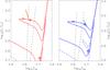Fig. 11

As Fig. 10, but with evolutionary tracks of standard (dashed) and overshooting (full) models for CEP-0227. The tracks are for the mean mass of the primary and upper mass limit for the secondary component. Standard and overshooting models are indicated at 138 and 157 Myr, respectively. The black dashed lines indicate the Cepheid instability strip according to Valle et al. (2009).

CEP-0227

is an EB where the primary is a Cepheid. Both stars have very similar masses of 4.16 ± 0.03 and 4.13 ± 0.04 M_⊙, which makes it almost trivial to find a common age within the errors. Consequently, this system was modelled successfully by Cassisi & Salaris (2011), Neilson & Langer (2012), and Prada Moroni et al. (2012). Based on the age-radius diagram alone, standard models also reproduce the radii at a common age (138 Myr). The temperature and luminosity ratios can also be fitted easily because of the rapid changes in these quantities during the fast post-MS evolution and by adjusting the mass by very small amounts. Only the blue loop of overshooting models, however, matches the observed luminosities and extends into the Cepheid regime. As already mentioned, we apply our description of overshooting for all convective zones. This leads to an increased luminosity due to core overshooting and an extended blue loop due to overshooting from the lower boundary of the surface convection zone. This is especially important for the modelling of Cepheids (see Cassisi 2004). With our standard overshooting parameter of f_ov = 0.02, we place the model at the upper arm of the blue loop, at an age of 157 Myr. These models also confirm that at that time the less massive star is in the Cepheid strip, while the more massive star is in the stable regime; see Fig. 11, where fits of the instability strip from Valle et al. (2009) are plotted with dashed black lines.

4.4. Additional systems

There are a number of additional detached eclipsed binary systems that have been widely investigated in the literature, but which we have not included. Here we discuss three of these systems and why we disregarded them.

TZ For is an EB consisting of two evolved stars with 2.05 ± 0.06 and 1.95 ± 0.03 M_⊙ (Andersen et al. 1991). Within these mass errors the evolutionary state of the primary is uncertain, as a common age can be found on the giant branch and during the core helium burning phase (see e.g. Andersen et al. 1991; Claret & Gimenez 1995; Claret 2011; Valle et al. 2017). Gallenne et al. (2016) reduced the mass uncertainties in this system significantly (2.057 ± 0.001 and 1.958 ± 0.001 M_⊙), which renders a fit of the primary on the giant branch impossible. In order for the primary to be in core helium burning, however, it is necessary that it underwent a core helium flash. The massive expansion prior to the helium flash, on the other hand, results in a radius that exceeds the orbit separation. In this case there was a phase of mass transfer and the assumption of co-evolution breaks down for TZ For. We therefore have disregarded TZ For.

α Cen is a well-studied binary for which precise determinations of masses (Pourbaix et al. 2002, 1.105 ± 0.007/0.934 ± 0.006 M_⊙) and radii (Kervella et al. 2003, 1.224 ± 0.003/0.863 ± 0.005 R_⊙) are available. Our models, however, yield an age for the secondary that is 25–50% lower than that of the primary. The problem seems to be that even though Kervella et al. (2003) claims an accuracy of 0.6% of the radius of the secondary, the log (g) measurement of Porto de Mello et al. (2008) suggests a much bigger radius. In fact, using the mean log (g) = 4.44 value of Porto de Mello et al. (2008) and the mass determined by Pourbaix et al. (2002), the estimated radius for the secondary would be 0.965 R_⊙, a difference of more than 20σ from the interferometric value by Kervella et al. (2003). With this radius the secondary would be considerably older than the primary, as can be seen in Porto de Mello et al. (2008) and Magic (2010). Seismic observations showed that α Cen A might have a convective core (Thévenin et al. 2002; Bazot et al. 2012, 2016). Our standard models do not support this claim while our diffusion models develop a small convective core shortly before the estimated age is reached. This would be consistent with the results of Bazot et al. (2016), who used Bayesian statistics to determine the properties of α Cen A and found a probability of 89% for a convective core if diffusion was considered in the models; however, these authors found that standard models with the updated ¹⁴N(p,γ)¹⁵O reaction rate (as in our models) had a very low probability for a convective core (2–3%). A clear indication for a convective core in α Cen A could therefore be another indication for the effectiveness of diffusion. At present, while this system has been well observed, there are still a number of open questions regarding both the observations and the models that prevent any conclusive modelling.

V432 Aur consists of a primary of 1.2 M_⊙ on the subgiant branch and a 1.1 M_⊙ MS companion (Siviero et al. 2004), which renders this system similar to V501 Her and AI Phe, but at a subsolar metallicity of [Fe/H] = −0.4. For this system, however, none of our models were able to give a common age. The age difference in the models increases when overshooting is included. Since stars in this mass range have very small convective cores, the mismatch of our models raises questions about our treatment of core overshooting for such cases.

5. Discussion

Table 4

Summary of our results.

We used detached eclipsing binaries as test objects for our stellar evolution code. This code is representative of current codes widely used and therefore our results should provide general conclusions about the quality of current stellar evolution theory and the physical assumptions employed. We concentrated in particular on the effects of overshooting from convective cores and atomic diffusion (mostly sedimentation), as it is used in standard solar model calculations. We summarize our results in Table 4, where we give the initial composition of our preferred models and the resulting age. At the given ages our models fit the observed radii and the temperature ratios of the systems. The age errors are due to the observed mass ranges given in Tables 1–3 and do not include errors due to the uncertainty in metallicity.

Diffusion.

Our models clearly show that diffusion has to be included to obtain accurate models for stars below ≈1.2 M_⊙ and an age ≳2 Gyr. Stars with higher masses have very thin convective envelopes, which makes the inclusion of diffusion difficult. Such envelopes get depleted of all metals almost instantaneously with our description, since we did not consider any additional effect that would act against the settling. Such additional effects are necessary because the abundances of carbon-enhanced (very) metal-poor stars (Matrozis & Stancliffe 2016), the abundance variations along globular cluster diagrams (e.g. Gruyters et al. 2013), or the level of the Li-Spite plateau (Richard et al. 2005) cannot be explained with uninhibited diffusion. Whether the counteracting mixing process is the postulated “turbulent diffusion” as in the latter paper, or simply mass loss (Vauclair & Charbonnel 1995), or any other process, remains to be clarified. For this reason we do not propose any conclusion for the higher mass objects.

The need for diffusion is especially evident in the open cluster NGC 6791, where fundamental parameters of the EBs V565 Lyr and V568 Lyr have been measured. Only models including diffusion result in a common age of both components in these systems. It is also the only possible way to match the individual surface metallicities with an identical initial composition. Additionally, the determined ages – close to 7 Gyr – of the two binary systems agree within 510 Myr, which is about the same level as the expected star formation time in this cluster according to Brogaard et al. (2012).

Brogaard et al. (2012) also considered diffusion in NGC 6791, but their result was less compelling than ours. While diffusion improved their fit in the mass – T_eff diagram (see their Fig. 7), they were no longer able to fit the V, B−V CMD and the V, V−I CMD simultaneously. They concluded that either diffusion or the colour-temperature transformations have to be improved. Our models including diffusion improved the match to the observed absolute temperatures as well. This is also the case for the two slightly more massive binaries UX Men and KOI-3571. However, we did not apply colour transformations, and therefore did not check whether we could reproduce colour-magnitude diagrams.

A more indirect argument for the presence of diffusion comes from the age of the system M55 V54 because standard models lead to an unreasonably large age. In the case of M55 V54 diffusion reduced the age from above 14 to ≈13.5 Gyr, in agreement with other age determinations of the globular cluster M55 (Dotter et al. 2010; Kaluzny et al. 2014). A similar conclusion was reached by Jofré & Weiss (2011), who compared the turn-off temperature of halo stars of the Sloan Digital Sky Survey with isochrones. They found that isochrones without diffusion need ages from 14–16 Gyr to fit the observations. Diffusive models reduced this age to 10–12 Gyr, in agreement with typical globular cluster ages. Our results add evidence regarding the effectiveness of particle sedimentation in low-mass star.

Overshooting.

Our models of main-sequence systems with convective cores in both binary components do not allow a firm conclusion about overshooting, as it is neither essential to model the systems, nor is it excluded. This is not unexpected because during most of the time on the MS overshooting has a small impact on the observable parameters. The situation changes with regard to the MS duration, since models without overshooting evolve to the subgiant branch earlier. Therefore, at the end of core hydrogen burning the age-radius diagram shows the biggest difference between overshooting and standard models. The primary of BG Ind is exactly at that point of its evolution and, as expected, only models with overshooting are able to fit the system. Beyond the MS, the evolution of overshooting and standard models is again very similar (but shifted in age and luminosity), which usually makes it hard to exclude standard models by the age-radius diagram alone. However, the increased luminosity of overshooting models leads to a different mass–luminosity relation. From our models it is clear that the higher luminosity makes it easier to fit systems beyond the MS. Examples are the cases of V2291 Oph, α Aur, and in particular the Cepheid binary Cep-0227. It is well known that the classical mass discrepancy for Cepheids can be solved by including convective overshooting on the main sequence (see e.g. Bono et al. 2001).

For MS stars the general need for overshooting in this mass range has been confirmed in other investigations, for example in Deheuvels et al. (2016), which is based on the seismology of 24 Kepler objects; only models including overshooting were able to reproduce the observed oscillation modes of main-sequence stars. Stancliffe et al. (2015), who modelled 12 double-lined EBs in a mass range from 1.3 to 6.2 M_⊙, also agree that overshooting is a necessity and that the general value of about 0.2 H_P provides a reasonable estimate. This is also in agreement with our standard choice.

The extent of the overshooting area around very small convective cores (stellar masses ≈1.2 M_⊙) is more uncertain. This is largely because overshooting descriptions usually depend on H_p, which diverges towards the stellar centre and would therefore predict unphysically large overshooting regions, exceeding by far the size of the convective core as determined by the canonical Schwarzschild criterion. In stellar evolution codes this problem is handled by various corrective measures, which lead to a cut-off of the overshooting area. Such a cut-off requires the additional calibration of the overshooting parameter in the mass range between 1.1–1.5 M_⊙, where convective cores typically appear. Some studies using eclipsing binaries (see e.g. Ribas et al. 2000; Claret 2007; Claret & Torres 2016) have suggested a mass-dependent overshooting parameter, while Stancliffe et al. (2015) have found no clear evidence for this. Valle et al. (2016) have actually concluded that it is currently not possible to calibrate f_ov with eclipsing binaries, in the mass range between 1.1 and 1.6 M_⊙, which they had investigated, because the uncertainty is of the order of the parameter itself. This study is based only on a synthetic sample of binary stars, and employs – as we do – also a fixed metallicity of the objects.

Our models do not give a clear answer to this question either. While overshooting cannot be excluded for UX Men, KOI-3571, and V501 Her, the most evolved system with that mass (AI Phe with 1.19 and 1.23 M_⊙) could not be fitted when overshooting (as applied by our own cut-off mechanism) was taken into account. Our selection of systems does not specifically probe the full critical mass range, but clusters around a mass of 1.2 M_⊙. The only other system with a slightly higher mass (1.3/1.4 M_⊙) is BG Ind. In this case, our treatment of overshooting from small convective cores allowed a reasonable fit to the system. Overall, we presently have no conclusive result about the growth of overshooting for small main-sequence masses. However, recently Hjørringgaard et al. (2017), using our code, have managed to model the star HD 185351 successfully in terms of reproducing all its properties obtained by interferometry, spectroscopy, and seismology only when applying our standard treatment of overshooting from the convective core. This star has a mass in excess of 1.5 M_⊙, and their model had a mass of 1.6 M_⊙.

To summarize, our study results in a slight preference for overshooting, as implemented in our code, and as such agrees with similar and independent studies.

Very low-mass stars.

Observations of low-mass stars show a discrepancy between estimated and modelled radii (see e.g. Hillenbrand & White 2004; Mann et al. 2015), where the models generally have 5−10% smaller radii than the observational estimates. The general problem of modelling such stars is the fact that the outer boundary condition influences the interior owing to the very deep convective envelopes. More sophisticated atmosphere models (see e.g. Baraffe et al. 1998) give an improved outer boundary condition, but are not able to resolve this problem. The outer boundary condition can also be altered by adding magnetic fields to the models, as has been carried out by Feiden (2016). Magnetic fields reduce the efficiency of convection, forcing the star to increase its radius in order to radiate its energy away. Indeed, López-Morales (2007) found that there is a clear correlation between stellar magnetic activity and the radius discrepancy in binary stars. A direct consequence of surface magnetic fields is the development of starspots. We added the effect of starspots to our models by including the model of Spruit & Weiss (1986). With this spot model, presented in Sect. 3.2, it is possible to inflate the radius of a star with a single parameter, which represents the effective spot coverage and can be chosen such that a common age for the system can be found. We used this approach to achieve common ages for the systems V636 Cen and Kepler 16 by inflating the secondary in these systems. The fully convective secondary of Kepler 16 needed only a very small spot coverage of 3% to match the age of its primary. V636 Cen on the other hand needed a huge spot coverage of 44%. This value is in the range of 35–51% found by Jackson & Jeffries (2014), who used a similar model to match polytropic models to six DDLEBs, the Pleiades, and the young cluster NGC 2516. Similar values have been found by O’Neal et al. (2004), who observed spot coverages of up to 42%. Even though this study observed stars with higher activity than the DDLEBs discussed here, it confirms that our results do not give unreasonably high values.

It should also be noted that spots introduce systematical errors in observations and therefore in the radii determinations. Windmiller et al. (2010) for example showed that spots on the EB GU Boo can lead to an error of up to 2% in interferometric radius determination, while the statistical errors from light curve fitting are reported with uncertainties of only 0.5–1%.

Mixing length α_MLT.

Throughout this study we used a solar calibrated mixing-length parameter α_MLT = 1.74, which is kept constant throughout all evolutionary phases and for all mass and metallicity values. We only modified α_MLT in the case of V2291 Oph because the models had lower temperatures than observed, and this discrepancy could not be explained by a change in composition. The simplest way to increase T_eff in these systems is to increase α_MLT. We needed at least α_MLT = 2.00 to match the observations. This is qualitatively in agreement with the general trend of an increasing α_MLT for post-main-sequence objects, as found by Trampedach et al. (2014) and Magic et al. (2015), where the entropy difference between the surface and the adiabatic interior of 3D-hydro atmospheres were matched by 1D-envelope models using the mixing-length description for convection with an adjustable parameter α_MLT. Although a solar-calibrated, constant α_MLT gives reasonable results in almost all of our cases, it is very evident that this parameter should be variable. However, we refrained from adding this additional degree of freedom in our models, as we did not encounter any clear need for it.

Further improvements.

Ignoring systematic errors from the observations, it is possible to precisely pin down the age of a given system for a given set of physics, by using the mass and radius determinations of DDLEBs. However, Lastennet & Valls-Gabaud (2002) showed that there exists a degeneracy between age and metallicity. This is especially important when we want to determine the necessary physics to model a system, where this degeneracy can also mask the results. The example of V501 Her showed that even small changes of ±0.05 dex in [Fe/H] can lead to different conclusions about the necessity for diffusion or overshooting. This is in fact to some degree the case for many of our objects: a much more accurate determination of the chemical composition is needed to draw firm conclusions about non-canonical physics effects. This was also emphasized by Young et al. (2001), along with the request for more accurate effective temperatures, a conclusion we agree to as well. It should be noted that the unknown helium content, which we have estimated with standard recipes based on global galactic chemical evolution wisdom, constitutes another fundamental and uncertain parameter. Because of the overlapping spectra of EBs, it is hard to achieve the required precision, but depending on the evolutionary state, an uncertainty of ±0.1 dex might be sufficient to put more stringent limitations on the necessary model physics. In relatively old systems with a low mass ratio it might be possible to give an estimate about the efficiency of diffusion, if such an accuracy can be achieved for both stars separately. An example of such a system is KOI-3571, for which our models indicate a difference of 0.09 dex in the surface metallicity.

Seismological data give further insight into the internal structure of stars. Well-chosen frequency ratios can help to determine the actual size of mixed stellar cores (see Silva Aguirre et al. 2011; Deheuvels et al. 2016). Combining this with the available observations can help to further restrict and thus improve the models.

6. Conclusions

We used the direct mass and radius determinations of 19 double-lined detached EBs to compare Garstec stellar evolution models with observations. We found that diffusive sedimentation of heavy elements has to be included in the models to reproduce the complete set of observables, which also includes the present surface abundances. Overshooting from convective areas is not necessary for those systems that still have both components on the MS, but overshooting has a stronger impact for more evolved stars at the end of the MS or beyond. The observables of most evolved systems in the intermediate mass range favour the inclusion of overshooting. The situation for stars with very small convective cores is more problematic, as the currently used descriptions diverge for these cases unless some additional restriction to the extent of the overshooting region is applied. With the geometrical cut-off implemented in Garstec we are able to fit successfully most systems, but in some cases our treatment fails. We also found some indications for a varying mixing-length parameter as was already suggested by 3D models. Finally, our model for starspots on the surface of very low-mass stars can resolve the differences in modelled and observed radii. In some cases, however, it requires a huge spot coverage, which reduces with increasing depth of the convective zone.

¹

http://www.astro.keele.ac.uk/jkt/debcat/

Acknowledgments

This work resulted from a master thesis (J.H.) at the Technical University, Munich. J.H. thanks D. D’Souza and G. Wagstaff for fruitful discussions. We also are grateful to G. Angelou for additional tests using his machine learning algorithm and for a critical reading of the manuscript. The referee has helped to improve the manuscript significantly with a very careful reading and constructive criticism. The additional improvement by the language editor is appreciated as well.

References

Alencar, S. H. P., Vaz, L. P. R., & Helt, B. E. 1997, A&A, 326, 709 [NASA ADS] [Google Scholar]
Andersen, J. 1991, A&ARv, 3, 91 [NASA ADS] [CrossRef] [Google Scholar]
Andersen, J., Clausen, J. V., Nordstrom, B., Gustafsson, B., & Vandenberg, D. A. 1988, A&A, 196, 128 [NASA ADS] [Google Scholar]
Andersen, J., Clausen, J. V., & Magain, P. 1989, A&A, 211, 346 [NASA ADS] [Google Scholar]
Andersen, J., Clausen, J. V., Nordstrom, B., Tomkin, J., & Mayor, M. 1991, A&A, 246, 99 [NASA ADS] [Google Scholar]
Angulo, C., Arnould, M., Rayet, M., et al. 1999, Nucl. Phys. A, 656, 3 [NASA ADS] [CrossRef] [Google Scholar]
Asplund, M., Grevesse, N., Sauval, A. J., & Scott, P. 2009, ARA&A, 47, 481 [NASA ADS] [CrossRef] [Google Scholar]
Bahcall, J. N., & Pinsonneault, M. H. 1992, Rev. Mod. Phys., 64, 885 [NASA ADS] [CrossRef] [Google Scholar]
Baraffe, I., Chabrier, G., Allard, F., & Hauschildt, P. H. 1998, A&A, 337, 403 [NASA ADS] [Google Scholar]
Bazot, M., Bourguignon, S., & Christensen-Dalsgaard, J. 2012, MNRAS, 427, 1847 [NASA ADS] [CrossRef] [Google Scholar]
Bazot, M., Christensen-Dalsgaard, J., Gizon, L., & Benomar, O. 2016, MNRAS, 460, 1254 [NASA ADS] [CrossRef] [Google Scholar]
Bono, G., Gieren, W. P., Marconi, M., Fouqué, P., & Caputo, F. 2001, ApJ, 563, 319 [NASA ADS] [CrossRef] [Google Scholar]
Bragaglia, A., Carretta, E., Gratton, R. G., et al. 2001, AJ, 121, 327 [NASA ADS] [CrossRef] [Google Scholar]
Brogaard, K., Bruntt, H., Grundahl, F., et al. 2011, A&A, 525, A2 [NASA ADS] [CrossRef] [EDP Sciences] [Google Scholar]
Brogaard, K., VandenBerg, D. A., Bruntt, H., et al. 2012, A&A, 543, A106 [NASA ADS] [CrossRef] [EDP Sciences] [Google Scholar]
Caffau, E., Ludwig, H.-G., Steffen, M., Freytag, B., & Bonifacio, P. 2011, Sol. Phys., 268, 255 [NASA ADS] [CrossRef] [Google Scholar]
Carraro, G., Villanova, S., Demarque, P., et al. 2006, ApJ, 643, 1151 [Google Scholar]
Carretta, E., Bragaglia, A., & Gratton, R. G. 2007, A&A, 473, 129 [NASA ADS] [CrossRef] [EDP Sciences] [Google Scholar]
Cassisi, S. 2004, in IAU Colloq. 193: Variable Stars in the Local Group, eds. D. W. Kurtz, & K. R. Pollard, ASP Conf. Ser., 310, 489 [Google Scholar]
Cassisi, S., & Salaris, M. 2011, ApJ, 728, L43 [NASA ADS] [CrossRef] [Google Scholar]
Chaboyer, B., Fenton, W. H., Nelan, J. E., Patnaude, D. J., & Simon, F. E. 2001, ApJ, 562, 521 [NASA ADS] [CrossRef] [Google Scholar]
Chiappini, C., Anders, F., Rodrigues, T. S., et al. 2015, A&A, 576, L12 [NASA ADS] [CrossRef] [EDP Sciences] [Google Scholar]
Claret, A. 2007, A&A, 475, 1019 [NASA ADS] [CrossRef] [EDP Sciences] [Google Scholar]
Claret, A. 2011, A&A, 526, A157 [NASA ADS] [CrossRef] [EDP Sciences] [Google Scholar]
Claret, A., & Gimenez, A. 1995, A&A, 296, 180 [NASA ADS] [Google Scholar]
Claret, A., & Torres, G. 2016, A&A, 592, A15 [NASA ADS] [CrossRef] [EDP Sciences] [Google Scholar]
Clausen, J. V., Bruntt, H., Claret, A., et al. 2009, A&A, 502, 253 [NASA ADS] [CrossRef] [EDP Sciences] [Google Scholar]
Cyburt, R. H., Fields, B. D., & Olive, K. A. 2008, JCAP, 11, 12 [Google Scholar]
Deheuvels, S., Brandão, I., Silva Aguirre, V., et al. 2016, A&A, 589, A93 [NASA ADS] [CrossRef] [EDP Sciences] [Google Scholar]
Dotter, A., Sarajedini, A., Anderson, J., et al. 2010, ApJ, 708, 698 [NASA ADS] [CrossRef] [Google Scholar]
Doyle, L. R., Carter, J. A., Fabrycky, D. C., et al. 2011, Science, 333, 1602 [NASA ADS] [CrossRef] [MathSciNet] [PubMed] [Google Scholar]
Feiden, G. A. 2016, A&A, 593, A99 [NASA ADS] [CrossRef] [EDP Sciences] [Google Scholar]
Feiden, G. A., & Chaboyer, B. 2012, ApJ, 757, 42 [NASA ADS] [CrossRef] [Google Scholar]
Feiden, G. A., & Chaboyer, B. 2014, ApJ, 789, 53 [NASA ADS] [CrossRef] [Google Scholar]
Ferguson, J. W., Alexander, D. R., Allard, F., et al. 2005, ApJ, 623, 585 [NASA ADS] [CrossRef] [Google Scholar]
Freytag, B., Ludwig, H.-G., & Steffen, M. 1996, A&A, 313, 497 [Google Scholar]
Gallenne, A., Pietrzyński, G., Graczyk, D., et al. 2016, A&A, 586, A35 [NASA ADS] [CrossRef] [EDP Sciences] [Google Scholar]
Garcia, E. V., Stassun, K. G., Pavlovski, K., et al. 2014, AJ, 148, 39 [NASA ADS] [CrossRef] [Google Scholar]
Gratton, R. G., Bonifacio, P., Bragaglia, A., et al. 2001, A&A, 369, 87 [NASA ADS] [CrossRef] [EDP Sciences] [Google Scholar]
Gratton, R., Bragaglia, A., Carretta, E., & Tosi, M. 2006, ApJ, 642, 462 [NASA ADS] [CrossRef] [Google Scholar]
Grevesse, N., & Noels, A. 1993, in Origin and Evolution of the Elements, eds. N. Prantzos, E. Vangioni-Flam, & M. Casse, 15 [Google Scholar]
Grevesse, N., & Sauval, A. J. 1998, Space Sci. Rev., 85, 161 [NASA ADS] [CrossRef] [Google Scholar]
Griffin, R. E. M., Marshall, K. P., Griffin, R. F., & Schroeder, K.-P. 1995, A&A, 301, 217 [NASA ADS] [Google Scholar]
Gruyters, P., Korn, A. J., Richard, O., et al. 2013, A&A, 555, A31 [NASA ADS] [CrossRef] [EDP Sciences] [Google Scholar]
Harris, W. E. 1996, AJ, 112, 1487 [NASA ADS] [CrossRef] [Google Scholar]
Hillenbrand, L. A., & White, R. J. 2004, ApJ, 604, 741 [NASA ADS] [CrossRef] [Google Scholar]
Hjørringgaard, J. G., Silva Aguirre, V., White, T. R., et al. 2017, MNRAS, 464, 3713 [NASA ADS] [CrossRef] [Google Scholar]
Iglesias, C. A., & Rogers, F. J. 1996, ApJ, 464, 943 [NASA ADS] [CrossRef] [Google Scholar]
Jackson, R. J., & Jeffries, R. D. 2014, MNRAS, 441, 2111 [NASA ADS] [CrossRef] [Google Scholar]
Jeffries, Jr., M. W., Sandquist, E. L., Mathieu, R. D., et al. 2013, AJ, 146, 58 [NASA ADS] [CrossRef] [Google Scholar]
Jofré, P., & Weiss, A. 2011, A&A, 533, A59 [NASA ADS] [CrossRef] [EDP Sciences] [Google Scholar]
Kaluzny, J., Thompson, I. B., Dotter, A., et al. 2014, Acta Astron., 64, 11 [NASA ADS] [Google Scholar]
Kervella, P., Thévenin, F., Ségransan, D., et al. 2003, A&A, 404, 1087 [NASA ADS] [CrossRef] [EDP Sciences] [Google Scholar]
Korn, A. J., Grundahl, F., Richard, O., et al. 2007, ApJ, 671, 402 [NASA ADS] [CrossRef] [Google Scholar]
Kraus, A. L., Tucker, R. A., Thompson, M. I., Craine, E. R., & Hillenbrand, L. A. 2011, ApJ, 728, 48 [NASA ADS] [CrossRef] [Google Scholar]
Lacy, C. H. S., Claret, A., & Sabby, J. A. 2004, AJ, 128, 1840 [NASA ADS] [CrossRef] [Google Scholar]
Lastennet, E., & Valls-Gabaud, D. 2002, A&A, 396, 551 [NASA ADS] [CrossRef] [EDP Sciences] [Google Scholar]
Lee-Brown, D. B., Anthony-Twarog, B. J., Deliyannis, C. P., Rich, E., & Twarog, B. A. 2015, AJ, 149, 121 [NASA ADS] [CrossRef] [Google Scholar]
López-Morales, M. 2007, ApJ, 660, 732 [NASA ADS] [CrossRef] [Google Scholar]
Magic, Z. 2010, Master’s thesis, Ludwig-Maximilians-Universität München [Google Scholar]
Magic, Z., Serenelli, A., Weiss, A., & Chaboyer, B. 2010, ApJ, 718, 1378 [NASA ADS] [CrossRef] [Google Scholar]
Magic, Z., Weiss, A., & Asplund, M. 2015, A&A, 573, A89 [NASA ADS] [CrossRef] [EDP Sciences] [Google Scholar]
Mann, A. W., Feiden, G. A., Gaidos, E., Boyajian, T., & von Braun, K. 2015, ApJ, 804, 64 [NASA ADS] [CrossRef] [Google Scholar]
Marshall, K. P. 1996, MNRAS, 280, 977 [NASA ADS] [CrossRef] [Google Scholar]
Marta, M., Formicola, A., Gyürky, G., et al. 2008, Phys. Rev. C, 78, 022802 [NASA ADS] [CrossRef] [Google Scholar]
Martig, M., Rix, H.-W., Aguirre, V. S., et al. 2015, MNRAS, 451, 2230 [NASA ADS] [CrossRef] [Google Scholar]
Matrozis, E., & Stancliffe, R. J. 2016, A&A, 592, A29 [NASA ADS] [CrossRef] [EDP Sciences] [Google Scholar]
Meng, Y., & Zhang, Q. S. 2014, ApJ, 787, 127 [NASA ADS] [CrossRef] [Google Scholar]
Miller Bertolami, M. M. 2016, A&A, 588, A25 [NASA ADS] [CrossRef] [EDP Sciences] [Google Scholar]
Molenda-Żakowicz, J., Brogaard, K., Niemczura, E., et al. 2014, MNRAS, 445, 2446 [NASA ADS] [CrossRef] [Google Scholar]
Neilson, H. R., & Langer, N. 2012, A&A, 537, A26 [NASA ADS] [CrossRef] [EDP Sciences] [Google Scholar]
O’Neal, D., Neff, J. E., Saar, S. H., & Cuntz, M. 2004, AJ, 128, 1802 [NASA ADS] [CrossRef] [Google Scholar]
Paquette, C., Pelletier, C., Fontaine, G., & Michaud, G. 1986, ApJS, 61, 177 [NASA ADS] [CrossRef] [Google Scholar]
Pavlovski, K., & Hensberge, H. 2005, A&A, 439, 309 [NASA ADS] [CrossRef] [EDP Sciences] [Google Scholar]
Pavlovski, K., & Southworth, J. 2009, MNRAS, 394, 1519 [NASA ADS] [CrossRef] [Google Scholar]
Peimbert, M., Luridiana, V., & Peimbert, A. 2007, ApJ, 666, 636 [NASA ADS] [CrossRef] [Google Scholar]
Peterson, R. C., & Green, E. M. 1998, ApJ, 502, L39 [NASA ADS] [CrossRef] [Google Scholar]
Pietrinferni, A., Cassisi, S., Salaris, M., & Castelli, F. 2004, ApJ, 612, 168 [NASA ADS] [CrossRef] [Google Scholar]
Pilecki, B., Graczyk, D., Pietrzyński, G., et al. 2013, MNRAS, 436, 953 [NASA ADS] [CrossRef] [Google Scholar]
Pols, O. R., Tout, C. A., Eggleton, P. P., & Han, Z. 1995, MNRAS, 274, 964 [NASA ADS] [CrossRef] [Google Scholar]
Pols, O. R., Tout, C. A., Schroder, K.-P., Eggleton, P. P., & Manners, J. 1997, MNRAS, 289, 869 [NASA ADS] [CrossRef] [Google Scholar]
Porto de Mello, G. F., Lyra, W., & Keller, G. R. 2008, A&A, 488, 653 [NASA ADS] [CrossRef] [EDP Sciences] [Google Scholar]
Pourbaix, D., Nidever, D., McCarthy, C., et al. 2002, A&A, 386, 280 [NASA ADS] [CrossRef] [EDP Sciences] [Google Scholar]
Prada Moroni, P. G., Gennaro, M., Bono, G., et al. 2012, ApJ, 749, 108 [NASA ADS] [CrossRef] [Google Scholar]
Ribas, I., Jordi, C., & Giménez, Á. 2000, MNRAS, 318, L55 [NASA ADS] [CrossRef] [Google Scholar]
Richard, O., Michaud, G., & Richer, J. 2005, ApJ, 619, 538 [NASA ADS] [CrossRef] [Google Scholar]
Rogers, F. J., & Nayfonov, A. 2002, ApJ, 576, 1064 [Google Scholar]
Romaniello, M., Primas, F., Mottini, M., et al. 2008, A&A, 488, 731 [NASA ADS] [CrossRef] [EDP Sciences] [Google Scholar]
Rozyczka, M., Kaluzny, J., Pych, W., et al. 2011, MNRAS, 414, 2479 [NASA ADS] [CrossRef] [Google Scholar]
Sandberg Lacy, C. H., & Fekel, F. C. 2014, AJ, 148, 71 [NASA ADS] [CrossRef] [Google Scholar]
Sandquist, E. L., Jessen-Hansen, J., Shetrone, M. D., et al. 2016, ApJ, 831, 11 [NASA ADS] [CrossRef] [Google Scholar]
Saumon, D., Chabrier, G., & van Horn, H. M. 1995, ApJS, 99, 713 [NASA ADS] [CrossRef] [Google Scholar]
Schlattl, H., & Weiss, A. 1999, A&A, 347, 272 [NASA ADS] [Google Scholar]
Schröder, K.-P., Pols, O. R., & Eggleton, P. P. 1997, MNRAS, 285, 696 [NASA ADS] [CrossRef] [Google Scholar]
Seaton, M. J., Yan, Y., Mihalas, D., & Pradhan, A. K. 1994, MNRAS, 266, 805 [NASA ADS] [CrossRef] [Google Scholar]
Silva Aguirre, V., Ballot, J., Serenelli, A. M., & Weiss, A. 2011, A&A, 529, A63 [NASA ADS] [CrossRef] [EDP Sciences] [Google Scholar]
Siviero, A., Munari, U., Sordo, R., et al. 2004, A&A, 417, 1083 [NASA ADS] [CrossRef] [EDP Sciences] [Google Scholar]
Southworth, J. 2015, in Living Together: Planets, Host Stars and Binaries, ASP Conf. Ser., 496, 164 [NASA ADS] [Google Scholar]
Southworth, J., Maxted, P. F. L., & Smalley, B. 2004, MNRAS, 351, 1277 [NASA ADS] [CrossRef] [Google Scholar]
Spruit, H. C., & Weiss, A. 1986, A&A, 166, 167 [NASA ADS] [Google Scholar]
Stancliffe, R. J., Fossati, L., Passy, J.-C., & Schneider, F. R. N. 2015, A&A, 575, A117 [NASA ADS] [CrossRef] [EDP Sciences] [Google Scholar]
Thévenin, F., Provost, J., Morel, P., et al. 2002, A&A, 392, L9 [NASA ADS] [CrossRef] [EDP Sciences] [Google Scholar]
Thoul, A. A., Bahcall, J. N., & Loeb, A. 1994, ApJ, 421, 828 [NASA ADS] [CrossRef] [Google Scholar]
Tkachenko, A., Degroote, P., Aerts, C., et al. 2014, MNRAS, 438, 3093 [NASA ADS] [CrossRef] [Google Scholar]
Torres, G., Andersen, J., & Giménez, A. 2010, A&ARv, 18, 67 [Google Scholar]
Torres, G., Claret, A., Pavlovski, K., & Dotter, A. 2015, ApJ, 807, 26 [NASA ADS] [CrossRef] [Google Scholar]
Trampedach, R., Stein, R. F., Christensen-Dalsgaard, J., Nordlund, Å., & Asplund, M. 2014, MNRAS, 445, 4366 [NASA ADS] [CrossRef] [Google Scholar]
Twarog, B. A., Carraro, G., & Anthony-Twarog, B. J. 2011, ApJ, 727, L7 [NASA ADS] [CrossRef] [Google Scholar]
Valle, G., Marconi, M., Degl’Innocenti, S., & Prada Moroni, P. G. 2009, A&A, 507, 1541 [NASA ADS] [CrossRef] [EDP Sciences] [Google Scholar]
Valle, G., Dell’Omodarme, M., Prada Moroni, P. G., & Degl’Innocenti, S. 2016, A&A, 587, A16 [NASA ADS] [CrossRef] [EDP Sciences] [Google Scholar]
Valle, G., Dell’Omodarme, M., Prada Moroni, P. G., & Degl’Innocenti, S. 2017, A&A, 600, A41 [NASA ADS] [CrossRef] [EDP Sciences] [Google Scholar]
Vauclair, S., & Charbonnel, C. 1995, A&A, 295, 715 [NASA ADS] [Google Scholar]
Villanova, S., Carraro, G., & Saviane, I. 2009, A&A, 504, 845 [NASA ADS] [CrossRef] [EDP Sciences] [Google Scholar]
Villante, F. L., Serenelli, A. M., Delahaye, F., & Pinsonneault, M. H. 2014, ApJ, 787, 13 [NASA ADS] [CrossRef] [Google Scholar]
Weiss, A. 1999, Habilitationsschrift, Ludwig-Maximilians-Universität München [Google Scholar]
Weiss, A., & Schlattl, H. 2008, Ap&SS, 316, 99 [NASA ADS] [CrossRef] [Google Scholar]
Windmiller, G., Orosz, J. A., & Etzel, P. B. 2010, ApJ, 712, 1003 [NASA ADS] [CrossRef] [Google Scholar]
Winn, J. N., Albrecht, S., Johnson, J. A., et al. 2011, ApJ, 741, L1 [NASA ADS] [CrossRef] [Google Scholar]
Worthey, G., & Jowett, K. J. 2003, PASP, 115, 96 [NASA ADS] [CrossRef] [Google Scholar]
Yakut, K., Eggleton, P. P., Kalomeni, B., Tout, C. A., & Eldridge, J. J. 2015, MNRAS, 453, 2937 [NASA ADS] [CrossRef] [Google Scholar]
Young, P. A., Mamajek, E. E., Arnett, D., & Liebert, J. 2001, ApJ, 556, 230 [NASA ADS] [CrossRef] [Google Scholar]
Zhang, Q. S. 2013, ApJS, 205, 18 [NASA ADS] [CrossRef] [Google Scholar]

All Tables

Table 1

Fundamental parameters of lower mass main-sequence systems (Sect. 4.1) ordered by increasing mass of the primary star A.

In the text

Table 2

As Table 1, but for more massive main-sequence systems with components that have a convective core.

In the text

Table 3

As Table 1, but for systems with components evolved past the main sequence.

In the text

Table 4

Summary of our results.

In the text

All Figures

Fig. 1

Model evolution of V565 Lyr. Horizontal areas with dashed central lines represent the observed error ranges. The solid line represents the evolution with the mean observed mass and the areas around it represent the 1σ mass range (see Table 1). The two panels show the radius evolution of the primary (top) and secondary (bottom) for V565 Lyr with [Fe/H] _i = 0.40, Y_i = 0.32. The models include diffusion. Within the errors a common age of 7.08 ± 0.15 Gyr is found (vertical lines).

In the text

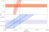	Fig. 2 As Fig. 1, but for V568 Lyr. The common age is 6.57 ± 0.14 Gyr.
In the text

	Fig. 3 Evolution of V636 Cen models. Same as the top two panels of Fig. 1, but for V636 Cen with [Fe/H] =−0.20, Y = 0.27 and an effective spot coverage of f_e = 0.33. In the lower panel, the additional black line shows the radius evolution of the secondary, if no spots are assumed.
In the text

Fig. 4

HRD of UX Men. Full lines show the evolutionary track of the models with diffusion and an initial metallicity of [Fe/H] _i = 0.2 and Y_i = 0.29. Dashed lines show tracks of standard models with the same mass, but without diffusion and a composition of [Fe/H] = 0.04, and Y = 0.28. All tracks are indicated at 2.1 Gyr. The red and blue shaded areas show the observational errors (as explained in Sect. 3.3) of primary (left panel) and secondary (right panel), respectively.

In the text

	Fig. 5 Models for BG Ind at [Fe/H] = −0.2; Y = 0.27, including overshooting. The panels are the same as in Fig. 1.
In the text

	Fig. 6 Same as in Fig. 1, but for KIC 9777062; the models include diffusion and overshooting. The composition is [Fe/H] _i = 0.04 and Y_i = 0.28.
In the text

	Fig. 7 Models for V453 Cyg, with a metallicity of [Fe/H] = −0.04; Y = 0.27, and allowing for overshooting. The black lines in the top two panels indicate the alternative evolution with standard physics, but [Fe/H] = −0.24.
In the text

	Fig. 8 As Fig. 5, but for standard models of V578 Mon with a metallicity of [Fe/H] = −0.17; Y = 0.27. The additional black lines indicate models of the mean mass with overshooting.
In the text

	Fig. 9 Evolution of [Fe/H] in AI Phe. The initial metallicity is assumed to be [Fe/H] _i = −0.04; Y_i = 0.27. The upper panel indicates the primary; the lower panel indicates the secondary component. The system age, indicated by the dashed line, is 4.681 ± 0.005 Gyr.
In the text

	Fig. 10 HRD of V2291 Oph models with [Fe/H] = 0.23; Y = 0.33 including overshooting and for cases with a mixing-length parameter of α_MLT = 1.74 (full) and α_MLT = 2.0 (dashed). The evolution of the primary is indicated by red and that of the secondary component by blue lines. Dashed and full lines are indicated at 183 and 180 Myr, respectively.
In the text

	Fig. 11 As Fig. 10, but with evolutionary tracks of standard (dashed) and overshooting (full) models for CEP-0227. The tracks are for the mean mass of the primary and upper mass limit for the secondary component. Standard and overshooting models are indicated at 138 and 157 Myr, respectively. The black dashed lines indicate the Cepheid instability strip according to Valle et al. (2009).
In the text

Current usage metrics show cumulative count of Article Views (full-text article views including HTML views, PDF and ePub downloads, according to the available data) and Abstracts Views on Vision4Press platform.

Data correspond to usage on the plateform after 2015. The current usage metrics is available 48-96 hours after online publication and is updated daily on week days.

Initial download of the metrics may take a while.

[1] Alencar, S. H. P., Vaz, L. P. R., & Helt, B. E. 1997, A&A, 326, 709 [NASA ADS] [Google Scholar]

[2] Andersen, J. 1991, A&ARv, 3, 91 [NASA ADS] [CrossRef] [Google Scholar]

[3] Andersen, J., Clausen, J. V., Nordstrom, B., Gustafsson, B., & Vandenberg, D. A. 1988, A&A, 196, 128 [NASA ADS] [Google Scholar]

[4] Andersen, J., Clausen, J. V., & Magain, P. 1989, A&A, 211, 346 [NASA ADS] [Google Scholar]

[5] Andersen, J., Clausen, J. V., Nordstrom, B., Tomkin, J., & Mayor, M. 1991, A&A, 246, 99 [NASA ADS] [Google Scholar]

[6] Angulo, C., Arnould, M., Rayet, M., et al. 1999, Nucl. Phys. A, 656, 3 [NASA ADS] [CrossRef] [Google Scholar]

[7] Asplund, M., Grevesse, N., Sauval, A. J., & Scott, P. 2009, ARA&A, 47, 481 [NASA ADS] [CrossRef] [Google Scholar]

[8] Bahcall, J. N., & Pinsonneault, M. H. 1992, Rev. Mod. Phys., 64, 885 [NASA ADS] [CrossRef] [Google Scholar]

[9] Baraffe, I., Chabrier, G., Allard, F., & Hauschildt, P. H. 1998, A&A, 337, 403 [NASA ADS] [Google Scholar]

[10] Bazot, M., Bourguignon, S., & Christensen-Dalsgaard, J. 2012, MNRAS, 427, 1847 [NASA ADS] [CrossRef] [Google Scholar]

[11] Bazot, M., Christensen-Dalsgaard, J., Gizon, L., & Benomar, O. 2016, MNRAS, 460, 1254 [NASA ADS] [CrossRef] [Google Scholar]

[12] Bono, G., Gieren, W. P., Marconi, M., Fouqué, P., & Caputo, F. 2001, ApJ, 563, 319 [NASA ADS] [CrossRef] [Google Scholar]

[13] Bragaglia, A., Carretta, E., Gratton, R. G., et al. 2001, AJ, 121, 327 [NASA ADS] [CrossRef] [Google Scholar]

[14] Brogaard, K., Bruntt, H., Grundahl, F., et al. 2011, A&A, 525, A2 [NASA ADS] [CrossRef] [EDP Sciences] [Google Scholar]

[15] Brogaard, K., VandenBerg, D. A., Bruntt, H., et al. 2012, A&A, 543, A106 [NASA ADS] [CrossRef] [EDP Sciences] [Google Scholar]

[16] Caffau, E., Ludwig, H.-G., Steffen, M., Freytag, B., & Bonifacio, P. 2011, Sol. Phys., 268, 255 [NASA ADS] [CrossRef] [Google Scholar]

[17] Carraro, G., Villanova, S., Demarque, P., et al. 2006, ApJ, 643, 1151 [Google Scholar]

[18] Carretta, E., Bragaglia, A., & Gratton, R. G. 2007, A&A, 473, 129 [NASA ADS] [CrossRef] [EDP Sciences] [Google Scholar]

[19] Cassisi, S. 2004, in IAU Colloq. 193: Variable Stars in the Local Group, eds. D. W. Kurtz, & K. R. Pollard, ASP Conf. Ser., 310, 489 [Google Scholar]

[20] Cassisi, S., & Salaris, M. 2011, ApJ, 728, L43 [NASA ADS] [CrossRef] [Google Scholar]

[21] Chaboyer, B., Fenton, W. H., Nelan, J. E., Patnaude, D. J., & Simon, F. E. 2001, ApJ, 562, 521 [NASA ADS] [CrossRef] [Google Scholar]

[22] Chiappini, C., Anders, F., Rodrigues, T. S., et al. 2015, A&A, 576, L12 [NASA ADS] [CrossRef] [EDP Sciences] [Google Scholar]

[23] Claret, A. 2007, A&A, 475, 1019 [NASA ADS] [CrossRef] [EDP Sciences] [Google Scholar]

[24] Claret, A. 2011, A&A, 526, A157 [NASA ADS] [CrossRef] [EDP Sciences] [Google Scholar]

[25] Claret, A., & Gimenez, A. 1995, A&A, 296, 180 [NASA ADS] [Google Scholar]

[26] Claret, A., & Torres, G. 2016, A&A, 592, A15 [NASA ADS] [CrossRef] [EDP Sciences] [Google Scholar]

[27] Clausen, J. V., Bruntt, H., Claret, A., et al. 2009, A&A, 502, 253 [NASA ADS] [CrossRef] [EDP Sciences] [Google Scholar]

[28] Cyburt, R. H., Fields, B. D., & Olive, K. A. 2008, JCAP, 11, 12 [Google Scholar]

[29] Deheuvels, S., Brandão, I., Silva Aguirre, V., et al. 2016, A&A, 589, A93 [NASA ADS] [CrossRef] [EDP Sciences] [Google Scholar]

[30] Dotter, A., Sarajedini, A., Anderson, J., et al. 2010, ApJ, 708, 698 [NASA ADS] [CrossRef] [Google Scholar]

[31] Doyle, L. R., Carter, J. A., Fabrycky, D. C., et al. 2011, Science, 333, 1602 [NASA ADS] [CrossRef] [MathSciNet] [PubMed] [Google Scholar]

[32] Feiden, G. A. 2016, A&A, 593, A99 [NASA ADS] [CrossRef] [EDP Sciences] [Google Scholar]

[33] Feiden, G. A., & Chaboyer, B. 2012, ApJ, 757, 42 [NASA ADS] [CrossRef] [Google Scholar]

[34] Feiden, G. A., & Chaboyer, B. 2014, ApJ, 789, 53 [NASA ADS] [CrossRef] [Google Scholar]

[35] Ferguson, J. W., Alexander, D. R., Allard, F., et al. 2005, ApJ, 623, 585 [NASA ADS] [CrossRef] [Google Scholar]

[36] Freytag, B., Ludwig, H.-G., & Steffen, M. 1996, A&A, 313, 497 [Google Scholar]

[37] Gallenne, A., Pietrzyński, G., Graczyk, D., et al. 2016, A&A, 586, A35 [NASA ADS] [CrossRef] [EDP Sciences] [Google Scholar]

[38] Garcia, E. V., Stassun, K. G., Pavlovski, K., et al. 2014, AJ, 148, 39 [NASA ADS] [CrossRef] [Google Scholar]

[39] Gratton, R. G., Bonifacio, P., Bragaglia, A., et al. 2001, A&A, 369, 87 [NASA ADS] [CrossRef] [EDP Sciences] [Google Scholar]

[40] Gratton, R., Bragaglia, A., Carretta, E., & Tosi, M. 2006, ApJ, 642, 462 [NASA ADS] [CrossRef] [Google Scholar]

[41] Grevesse, N., & Noels, A. 1993, in Origin and Evolution of the Elements, eds. N. Prantzos, E. Vangioni-Flam, & M. Casse, 15 [Google Scholar]

[42] Grevesse, N., & Sauval, A. J. 1998, Space Sci. Rev., 85, 161 [NASA ADS] [CrossRef] [Google Scholar]

[43] Griffin, R. E. M., Marshall, K. P., Griffin, R. F., & Schroeder, K.-P. 1995, A&A, 301, 217 [NASA ADS] [Google Scholar]

[44] Gruyters, P., Korn, A. J., Richard, O., et al. 2013, A&A, 555, A31 [NASA ADS] [CrossRef] [EDP Sciences] [Google Scholar]

[45] Harris, W. E. 1996, AJ, 112, 1487 [NASA ADS] [CrossRef] [Google Scholar]

[46] Hillenbrand, L. A., & White, R. J. 2004, ApJ, 604, 741 [NASA ADS] [CrossRef] [Google Scholar]

[47] Hjørringgaard, J. G., Silva Aguirre, V., White, T. R., et al. 2017, MNRAS, 464, 3713 [NASA ADS] [CrossRef] [Google Scholar]

[48] Iglesias, C. A., & Rogers, F. J. 1996, ApJ, 464, 943 [NASA ADS] [CrossRef] [Google Scholar]

[49] Jackson, R. J., & Jeffries, R. D. 2014, MNRAS, 441, 2111 [NASA ADS] [CrossRef] [Google Scholar]

[50] Jeffries, Jr., M. W., Sandquist, E. L., Mathieu, R. D., et al. 2013, AJ, 146, 58 [NASA ADS] [CrossRef] [Google Scholar]

[51] Jofré, P., & Weiss, A. 2011, A&A, 533, A59 [NASA ADS] [CrossRef] [EDP Sciences] [Google Scholar]

[52] Kaluzny, J., Thompson, I. B., Dotter, A., et al. 2014, Acta Astron., 64, 11 [NASA ADS] [Google Scholar]

[53] Kervella, P., Thévenin, F., Ségransan, D., et al. 2003, A&A, 404, 1087 [NASA ADS] [CrossRef] [EDP Sciences] [Google Scholar]

[54] Korn, A. J., Grundahl, F., Richard, O., et al. 2007, ApJ, 671, 402 [NASA ADS] [CrossRef] [Google Scholar]

[55] Kraus, A. L., Tucker, R. A., Thompson, M. I., Craine, E. R., & Hillenbrand, L. A. 2011, ApJ, 728, 48 [NASA ADS] [CrossRef] [Google Scholar]

[56] Lacy, C. H. S., Claret, A., & Sabby, J. A. 2004, AJ, 128, 1840 [NASA ADS] [CrossRef] [Google Scholar]

[57] Lastennet, E., & Valls-Gabaud, D. 2002, A&A, 396, 551 [NASA ADS] [CrossRef] [EDP Sciences] [Google Scholar]

[58] Lee-Brown, D. B., Anthony-Twarog, B. J., Deliyannis, C. P., Rich, E., & Twarog, B. A. 2015, AJ, 149, 121 [NASA ADS] [CrossRef] [Google Scholar]

[59] López-Morales, M. 2007, ApJ, 660, 732 [NASA ADS] [CrossRef] [Google Scholar]

[60] Magic, Z. 2010, Master’s thesis, Ludwig-Maximilians-Universität München [Google Scholar]

[61] Magic, Z., Serenelli, A., Weiss, A., & Chaboyer, B. 2010, ApJ, 718, 1378 [NASA ADS] [CrossRef] [Google Scholar]

[62] Magic, Z., Weiss, A., & Asplund, M. 2015, A&A, 573, A89 [NASA ADS] [CrossRef] [EDP Sciences] [Google Scholar]

[63] Mann, A. W., Feiden, G. A., Gaidos, E., Boyajian, T., & von Braun, K. 2015, ApJ, 804, 64 [NASA ADS] [CrossRef] [Google Scholar]

[64] Marshall, K. P. 1996, MNRAS, 280, 977 [NASA ADS] [CrossRef] [Google Scholar]

[65] Marta, M., Formicola, A., Gyürky, G., et al. 2008, Phys. Rev. C, 78, 022802 [NASA ADS] [CrossRef] [Google Scholar]

[66] Martig, M., Rix, H.-W., Aguirre, V. S., et al. 2015, MNRAS, 451, 2230 [NASA ADS] [CrossRef] [Google Scholar]

[67] Matrozis, E., & Stancliffe, R. J. 2016, A&A, 592, A29 [NASA ADS] [CrossRef] [EDP Sciences] [Google Scholar]

[68] Meng, Y., & Zhang, Q. S. 2014, ApJ, 787, 127 [NASA ADS] [CrossRef] [Google Scholar]

[69] Miller Bertolami, M. M. 2016, A&A, 588, A25 [NASA ADS] [CrossRef] [EDP Sciences] [Google Scholar]

[70] Molenda-Żakowicz, J., Brogaard, K., Niemczura, E., et al. 2014, MNRAS, 445, 2446 [NASA ADS] [CrossRef] [Google Scholar]

[71] Neilson, H. R., & Langer, N. 2012, A&A, 537, A26 [NASA ADS] [CrossRef] [EDP Sciences] [Google Scholar]

[72] O’Neal, D., Neff, J. E., Saar, S. H., & Cuntz, M. 2004, AJ, 128, 1802 [NASA ADS] [CrossRef] [Google Scholar]

[73] Paquette, C., Pelletier, C., Fontaine, G., & Michaud, G. 1986, ApJS, 61, 177 [NASA ADS] [CrossRef] [Google Scholar]

[74] Pavlovski, K., & Hensberge, H. 2005, A&A, 439, 309 [NASA ADS] [CrossRef] [EDP Sciences] [Google Scholar]

[75] Pavlovski, K., & Southworth, J. 2009, MNRAS, 394, 1519 [NASA ADS] [CrossRef] [Google Scholar]

[76] Peimbert, M., Luridiana, V., & Peimbert, A. 2007, ApJ, 666, 636 [NASA ADS] [CrossRef] [Google Scholar]

[77] Peterson, R. C., & Green, E. M. 1998, ApJ, 502, L39 [NASA ADS] [CrossRef] [Google Scholar]

[78] Pietrinferni, A., Cassisi, S., Salaris, M., & Castelli, F. 2004, ApJ, 612, 168 [NASA ADS] [CrossRef] [Google Scholar]

[79] Pilecki, B., Graczyk, D., Pietrzyński, G., et al. 2013, MNRAS, 436, 953 [NASA ADS] [CrossRef] [Google Scholar]

[80] Pols, O. R., Tout, C. A., Eggleton, P. P., & Han, Z. 1995, MNRAS, 274, 964 [NASA ADS] [CrossRef] [Google Scholar]

[81] Pols, O. R., Tout, C. A., Schroder, K.-P., Eggleton, P. P., & Manners, J. 1997, MNRAS, 289, 869 [NASA ADS] [CrossRef] [Google Scholar]

[82] Porto de Mello, G. F., Lyra, W., & Keller, G. R. 2008, A&A, 488, 653 [NASA ADS] [CrossRef] [EDP Sciences] [Google Scholar]

[83] Pourbaix, D., Nidever, D., McCarthy, C., et al. 2002, A&A, 386, 280 [NASA ADS] [CrossRef] [EDP Sciences] [Google Scholar]

[84] Prada Moroni, P. G., Gennaro, M., Bono, G., et al. 2012, ApJ, 749, 108 [NASA ADS] [CrossRef] [Google Scholar]

[85] Ribas, I., Jordi, C., & Giménez, Á. 2000, MNRAS, 318, L55 [NASA ADS] [CrossRef] [Google Scholar]

[86] Richard, O., Michaud, G., & Richer, J. 2005, ApJ, 619, 538 [NASA ADS] [CrossRef] [Google Scholar]

[87] Rogers, F. J., & Nayfonov, A. 2002, ApJ, 576, 1064 [Google Scholar]

[88] Romaniello, M., Primas, F., Mottini, M., et al. 2008, A&A, 488, 731 [NASA ADS] [CrossRef] [EDP Sciences] [Google Scholar]

[89] Rozyczka, M., Kaluzny, J., Pych, W., et al. 2011, MNRAS, 414, 2479 [NASA ADS] [CrossRef] [Google Scholar]

[90] Sandberg Lacy, C. H., & Fekel, F. C. 2014, AJ, 148, 71 [NASA ADS] [CrossRef] [Google Scholar]

[91] Sandquist, E. L., Jessen-Hansen, J., Shetrone, M. D., et al. 2016, ApJ, 831, 11 [NASA ADS] [CrossRef] [Google Scholar]

[92] Saumon, D., Chabrier, G., & van Horn, H. M. 1995, ApJS, 99, 713 [NASA ADS] [CrossRef] [Google Scholar]

[93] Schlattl, H., & Weiss, A. 1999, A&A, 347, 272 [NASA ADS] [Google Scholar]

[94] Schröder, K.-P., Pols, O. R., & Eggleton, P. P. 1997, MNRAS, 285, 696 [NASA ADS] [CrossRef] [Google Scholar]

[95] Seaton, M. J., Yan, Y., Mihalas, D., & Pradhan, A. K. 1994, MNRAS, 266, 805 [NASA ADS] [CrossRef] [Google Scholar]

[96] Silva Aguirre, V., Ballot, J., Serenelli, A. M., & Weiss, A. 2011, A&A, 529, A63 [NASA ADS] [CrossRef] [EDP Sciences] [Google Scholar]

[97] Siviero, A., Munari, U., Sordo, R., et al. 2004, A&A, 417, 1083 [NASA ADS] [CrossRef] [EDP Sciences] [Google Scholar]

[98] Southworth, J. 2015, in Living Together: Planets, Host Stars and Binaries, ASP Conf. Ser., 496, 164 [NASA ADS] [Google Scholar]

[99] Southworth, J., Maxted, P. F. L., & Smalley, B. 2004, MNRAS, 351, 1277 [NASA ADS] [CrossRef] [Google Scholar]

[100] Spruit, H. C., & Weiss, A. 1986, A&A, 166, 167 [NASA ADS] [Google Scholar]

[101] Stancliffe, R. J., Fossati, L., Passy, J.-C., & Schneider, F. R. N. 2015, A&A, 575, A117 [NASA ADS] [CrossRef] [EDP Sciences] [Google Scholar]

[102] Thévenin, F., Provost, J., Morel, P., et al. 2002, A&A, 392, L9 [NASA ADS] [CrossRef] [EDP Sciences] [Google Scholar]

[103] Thoul, A. A., Bahcall, J. N., & Loeb, A. 1994, ApJ, 421, 828 [NASA ADS] [CrossRef] [Google Scholar]

[104] Tkachenko, A., Degroote, P., Aerts, C., et al. 2014, MNRAS, 438, 3093 [NASA ADS] [CrossRef] [Google Scholar]

[105] Torres, G., Andersen, J., & Giménez, A. 2010, A&ARv, 18, 67 [Google Scholar]

[106] Torres, G., Claret, A., Pavlovski, K., & Dotter, A. 2015, ApJ, 807, 26 [NASA ADS] [CrossRef] [Google Scholar]

[107] Trampedach, R., Stein, R. F., Christensen-Dalsgaard, J., Nordlund, Å., & Asplund, M. 2014, MNRAS, 445, 4366 [NASA ADS] [CrossRef] [Google Scholar]

[108] Twarog, B. A., Carraro, G., & Anthony-Twarog, B. J. 2011, ApJ, 727, L7 [NASA ADS] [CrossRef] [Google Scholar]

[109] Valle, G., Marconi, M., Degl’Innocenti, S., & Prada Moroni, P. G. 2009, A&A, 507, 1541 [NASA ADS] [CrossRef] [EDP Sciences] [Google Scholar]

[110] Valle, G., Dell’Omodarme, M., Prada Moroni, P. G., & Degl’Innocenti, S. 2016, A&A, 587, A16 [NASA ADS] [CrossRef] [EDP Sciences] [Google Scholar]

[111] Valle, G., Dell’Omodarme, M., Prada Moroni, P. G., & Degl’Innocenti, S. 2017, A&A, 600, A41 [NASA ADS] [CrossRef] [EDP Sciences] [Google Scholar]

[112] Vauclair, S., & Charbonnel, C. 1995, A&A, 295, 715 [NASA ADS] [Google Scholar]

[113] Villanova, S., Carraro, G., & Saviane, I. 2009, A&A, 504, 845 [NASA ADS] [CrossRef] [EDP Sciences] [Google Scholar]

[114] Villante, F. L., Serenelli, A. M., Delahaye, F., & Pinsonneault, M. H. 2014, ApJ, 787, 13 [NASA ADS] [CrossRef] [Google Scholar]

[115] Weiss, A. 1999, Habilitationsschrift, Ludwig-Maximilians-Universität München [Google Scholar]

[116] Weiss, A., & Schlattl, H. 2008, Ap&SS, 316, 99 [NASA ADS] [CrossRef] [Google Scholar]

[117] Windmiller, G., Orosz, J. A., & Etzel, P. B. 2010, ApJ, 712, 1003 [NASA ADS] [CrossRef] [Google Scholar]

[118] Winn, J. N., Albrecht, S., Johnson, J. A., et al. 2011, ApJ, 741, L1 [NASA ADS] [CrossRef] [Google Scholar]

[119] Worthey, G., & Jowett, K. J. 2003, PASP, 115, 96 [NASA ADS] [CrossRef] [Google Scholar]

[120] Yakut, K., Eggleton, P. P., Kalomeni, B., Tout, C. A., & Eldridge, J. J. 2015, MNRAS, 453, 2937 [NASA ADS] [CrossRef] [Google Scholar]

[121] Young, P. A., Mamajek, E. E., Arnett, D., & Liebert, J. 2001, ApJ, 556, 230 [NASA ADS] [CrossRef] [Google Scholar]

[122] Zhang, Q. S. 2013, ApJS, 205, 18 [NASA ADS] [CrossRef] [Google Scholar]

Testing stellar evolution models with detached eclipsing binaries

1. Introduction

2. Observational data

3. Stellar models and procedure

3.1. Canonical model assumptions

3.2. Additional physical options

Convective overshooting.

Atomic diffusion.

Stellar spot model.

3.3. Procedure

4. Results

4.1. Main-sequence systems: M < 1.1 M⊙

V565 Lyr and V568 Lyr.

M55 V54.

V636 Cen.

Kepler-16

4.2. Main-sequence systems: M > 1.2 M⊙

UX Men and KOI-3571.

BG Ind

KIC 9777062

MU Cas and V906 Sco.

V453 Cyg.

V380 Cyg.

V578 Mon.

4.3. Evolved systems

AI Phe.

V501 Her

V2291 Oph

α Aur

CEP-0227

4.4. Additional systems

5. Discussion

Diffusion.

Overshooting.

Very low-mass stars.

Mixing length αMLT.

Further improvements.

6. Conclusions

Acknowledgments

References

All Tables

All Figures

4.1. Main-sequence systems: M < 1.1 M_⊙

4.2. Main-sequence systems: M > 1.2 M_⊙

Mixing length α_MLT.