| Issue |
A&A
Volume 606, October 2017
|
|
|---|---|---|
| Article Number | A129 | |
| Number of page(s) | 8 | |
| Section | Numerical methods and codes | |
| DOI | https://doi.org/10.1051/0004-6361/201731248 | |
| Published online | 24 October 2017 | |
Equation of state SAHA-S meets stellar evolution code CESAM2k
1 Sternberg Astronomical Institute, Lomonosov Moscow State University, 119234 Moscow, Russia
e-mail: This email address is being protected from spambots. You need JavaScript enabled to view it.
2 Department of Physics and Astronomy, University of Southern California, Los Angeles, CA 90089, USA
3 Université de La Côte d’Azur, OCA, Laboratoire Lagrange CNRS, BP 4229, 06304 Nice Cedex, France
4 Institute of Problems of Chemical Physics RAS, 142432 Chernogolovka, Russia
5 Tomsk State University, 634050 Tomsk, Russia
6 Joint Institute for High Temperatures RAS, 125412 Moscow, Russia
7 Moscow Institute of Physics and Technology, 141701 Dolgoprudnyi, Russia
8 Troitsk Institute for Innovation and Fusion Research, 142190 Troitsk, Russia
Received: 26 May 2017
Accepted: 1 August 2017
Abstract
Context. We present an example of an interpolation code of the SAHA-S equation of state that has been adapted for use in the stellar evolution code CESAM2k.
Aims. The aim is to provide the necessary data and numerical procedures for its implementation in a stellar code. A technical problem is the discrepancy between the sets of thermodynamic quantities provided by the SAHA-S equation of state and those necessary in the CESAM2k computations. Moreover, the independent variables in a practical equation of state (like SAHA-S) are temperature and density, whereas for modelling calculations the variables temperature and pressure are preferable. Specifically for the CESAM2k code, some additional quantities and their derivatives must be provided.
Methods. To provide the bridge between the equation of state and stellar modelling, we prepare auxiliary tables of the quantities that are demanded in CESAM2k. Then we use cubic spline interpolation to provide both smoothness and a good approximation of the necessary derivatives. Using the B-form of spline representation provides us with an efficient algorithm for three-dimensional interpolation.
Results. The table of B-spline coefficients provided can be directly used during stellar model calculations together with the module of cubic spline interpolation. This implementation of the SAHA-S equation of state in the CESAM2k stellar structure and evolution code has been tested on a solar model evolved to the present. A comparison with other equations of state is briefly discussed.
Conclusions. The choice of a regular net of mesh points for specific primary quantities in the SAHA-S equation of state, together with accurate and consistently smooth tabulated values, provides an effective algorithm of interpolation in modelling calculations. The proposed module of interpolation procedures can be easily adopted in other evolution codes.
Key words: equation of state / methods: numerical / Sun: evolution / Sun: interior / stars: evolution / stars: interiors
© ESO, 2017
1. Introduction
One of the most important factors for successfully modelling the stellar-interior structure is the equation of state (EOS) of the matter. It governs both the opacity and the thermodynamic structure of the star, which determine the predictions of the models, such as the surface temperature, luminosity, and radius for a given age of the star. For several decades, several EOS formalisms have been tested in evolutionary models of different kinds of stars, mainly depending on mass and chemical composition. For example, in the CESAM2k code (Morel & Lebreton 2008) different EOS can be considered, such as OPAL (Rogers et al. 1996; Rogers & Nayfonov 2002) or the MHD EOS (Mihalas et al. 1988); the code has been extensively used to reproduce the Sun as a star (Morel et al. 1997) as well as many other stars of different mass and chemical composition as a function of age.
In this paper we describe the implementation of the recently developed EOS named SAHA-S (Gryaznov et al. 2006, 2013) in the CESAM2k code and provide examples of its capability to reproduce the Sun as a star. In Sect. 2 we describe basic concepts and relations of EOS theory. The requirements by CESAM2k on the EOS are listed in Sect. 3, and the corresponding available SAHA-S data are discussed in Sect. 4. Implementation of the SAHA-S EOS in the mathematical structure of the CESAM2k code is described in Sect. 5. Particular attention is given to the numerical algorithms based on a three-dimensional cubic spline interpolation (de Boor 1978). In Sect. 6, we show how some physical quantities such as the sound speed profile in the interior are reproduced in a solar model based on the SAHA-S EOS, and we make comparisons with earlier CESAM2k models that were based on the OPAL EOS. Conclusions are presented in Sect. 7.
2. Basic concepts and relations
For matter in thermodynamical equilibrium, the EOS is the relation between pressure P, temperature T, and density ρ, assuming a fixed chemical composition. There are many introductions into the EOS and its role in modelling stellar structure (e.g. Cox & Giuli 1968; Hansen & Kawaler 1994). However, recent computations of the EOS based on more modern physical assumptions have therefore become very difficult and elaborate (see e.g. Gryaznov et al. 2006, 2013, for the case of the SAHA-S EOS).
2.1. Geometry of EOS
Mathematically speaking, in the coordinate space { P,T,ρ }, an EOS can be represented as a surface (two-dimensional manifold). For a given mass and chemical composition, any change in the thermodynamic state is described by a curve on this surface. In models of stellar internal structure, a given trace inside the star is associated with quantities { P,T,ρ } that lie on this EOS surface.
From a geometrical point of view, the EOS surface is a smooth (differentiable) surface. This leads to the next geometrical structure, a tangent plane which uniquely exists at every point of the surface. To describe and define the tangent plane (which is a linear space), we write an expression for differential of pressure in the form  (1)
(1)
Following historical tradition in astrophysics, we use logarithmic variables wherever possible. In the differential of pressure, two dimensionless partial derivatives appear as (2)These derivatives essentially describe the orientation of the tangent plane in the coordinate space. χT = χρ = 1 for a perfect-gas EOS, at least in some finite part of the EOS surface, and there the scaled pressure
  (3)is constant. As a pure geometrical consequence, a third partial derivative δ can be introduced, and it is related to the two derivatives defined above:
  (4)Here we provide a definition of the tangent plane with help of the pressure differential because it is the most natural for a thermodynamic description in which T and ρ are the independent variables. However, for applications to stellar modelling, the differential of density is more useful because T and P are the independent variables. Obviously, again geometrically, one can write
  (5)
(5)
From this expression it becomes clear why δ and  are needed in stellar evolution codes, and in CESAM2k in particular.
This picture can be generalized to the case where the coordinate space has more dimensions, as in the case of a non-constant chemical composition. This simple case is expressed by X and Z, which are respectively the mass fractions of hydrogen and all elements heavier than helium. With additional partial derivatives  (6)the differential of density becomes
  (7)The last derivative with respect to Z is smaller than the derivative with respect to X and we omit it in further expressions.
The practical meaning of the tangent plane might not be obvious until we actually deal with the principal task in the theory of the EOS. Nevertheless, let us consider here the case where a curve C in the EOS surface passes through the point M characterized by the temperature-density pair T,ρ. Then there is a tangent line to the curve C at this point M. This tangent line is also part of the tangent plane of the EOS surface originating at the point M. If we know one coordinate projection of the tangent line, this means that we can deduce the two other projections as well.
In the next chapter, we consider an important illustration of this problem (the adiabatic process).
2.2. Adiabatic gradients
The fundamental thermodynamic laws state that there is a unique curve of an isentropic process for each point of the EOS, and again the direction of adiabatic changes belongs to the tangent plane of that point. Generally, adiabatic changes performed under constant chemical composition are considered. The adiabatic direction can be determined by any of the three projections on the coordinate planes. Conventionally, the best-known notations for them are ![Mathematical equation: \begin{eqnarray} &&{\Gamma _1} \equiv {\left. {\frac{{\partial\!\ln P}}{{\partial\!\ln \rho }}} \right|_{\rm S}}, \\[3mm] &&{\nabla _{{\mathrm{ad}}}} \equiv {\left. {\frac{{\partial\!\ln T}}{{\partial\!\ln P}}} \right|_{\rm S}}, \\[3mm] &&{\Gamma _3} - 1 \equiv {\left. {\frac{{\partial\!\ln T}}{{\partial\!\ln \rho }}} \right|_{\rm S}} , \end{eqnarray}](/articles/aa/full_html/2017/10/aa31248-17/aa31248-17-eq20.png) where ∇ad is the standard notation for the adiabatic temperature gradient, while the notations Γ1 and Γ3−1 refer to S. Chandrasekhar (Chandrasekhar 1939; Lang 1974; or Cox & Giuli 1968; Weiss et al. 2004). The three derivatives are obviously related
where ∇ad is the standard notation for the adiabatic temperature gradient, while the notations Γ1 and Γ3−1 refer to S. Chandrasekhar (Chandrasekhar 1939; Lang 1974; or Cox & Giuli 1968; Weiss et al. 2004). The three derivatives are obviously related  (11)However, to obtain any of these adiabatic projections additional thermodynamic information is required. The most natural way is based on the caloric EOS, expressed through
  (12)where Π is defined by Eq. (3), cV is the specific heat capacity at constant volume
  (13)If the adiabatic projection Γ3−1 is found, the other two become
  (14)and
  (15)The value of ∇ad is fundamental for modelling stellar convection zones, whereas Γ1 is directly related to the adiabatic sound speed c2 = Γ1P/ρ, which is necessary for seismic calculations. Also, there is a direct relation between Γ1 and ∇ad without recourse to Γ3−1:
  (16)In addition to cV, another caloric quantity is cP, the specific heat capacity under constant pressure:
  (17)A common way to calculate cP is by using the difference between the two capacities, which is solely a consequence of the geometry of the EOS surface:
  (18)Then the adiabatic exponents are
  (19)and
  (20)In summary, the minimum necessary thermodynamic information is given by the three quantities P, χT, χρ, and by one of four quantities (cV,cP,∇ad,Γ1). Specifically, the stellar evolution code CESAM2k requires the data set
  , which can be obtained from that set of thermodynamic quantities.
2.3. Trace of the stellar model on the EOS surface
To avoid going into too much detail about the modelling procedure, here we outline only the general scheme. The modelling is principally based on equations giving ∇P and ∇T as functions of T,ρ,X,Z at every point. The goal of the procedure is to obtain a model curve CM, expressed as the parametric functions  , where r is radial coordinate in the model. This curve belongs to the general EOS surface in {PTρ;XZ} space. The derivative along the radius of the model curve CM
 (21)depends not only on local thermodynamic values, but also on model parameters. Therefore, the individual points on the model curve can only be determined as a result of the calculation of the entire model.
The spatial derivative of the density dρ/ dr is necessary for the calculation of the square of the Brunt-Väisälä frequency  , which together with the square of the sound speed
  ,
,  (22)constitutes the principal parameters defining the oscillation properties of the model. By definition (Unno et al. 1989),
  (23)where g is the gravitational acceleration. Using spatial derivatives in the model
 (24)we can write
 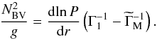 (25)The structure of is similar to the structure of ∇M (Eq. (21)), except that in the case of we also need the gradient of density ∇ρ in the model, but ∇ρ is not directly available, in contrast to ∇P and ∇T which are the part of the modelling procedure. There are two ways to get ∇ρ. One is by direct numerical differentiation of model profile ρ(r), but that may be numerically unstable. Another way is by expression of the thermodynamical differential for density (7). Then an expression for can be obtained in the form
 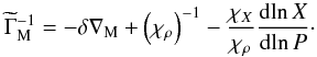 (26)In deriving Eq. (26) from Eq. (7), we have omitted the last term in (7), containing the derivative of pressure with respect to Z, i.e. χZ. Nevertheless, we still use and need the derivative of pressure χX, together with the gradient of X(r) from the model data.
Generally, the gradient of X is a much more slowly varying function than the gradient of ρ. In several important regions of the star it is equal to or close to zero. For example, in the mixed and chemically homogeneous convection zone, the following expression for can be used 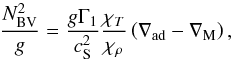 (27)where Eqs. (16) and (5) have been taken into account. In the convection zone, expression (27) is much more stable and virtually exact when compared with the same quantity obtained by numerical differentiation. The reason is that the difference (∇ad−∇M) is very small in most places in the convection zone, and in addition is directly provided by convective transport equation. However, Eq. (26) is so far not used in CESAM2k, and Eq. (23) is used in the convection zone and in other parts of the star.
2.4. Calculation of gravitational energy contribution
In calculations of stellar evolutions, the contribution from the release of gravitational energy is significant, especially on the pre-main sequence stage. It is calculated on the basis of the formula 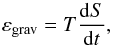 (28)where
  (29)
(29)
The computation of dU requires the internal energy U from the EOS.
3. Requirements of CESAM2k regarding the thermodynamic quantities of the EOS
The stellar evolution code CESAM2k (Morel & Lebreton 2008) calls for an EOS in the form of ρ = ρ(P,T), i.e. with pressure P and temperature T as the independent variables. Further input parameters for the physical quantities are the hydrogen mass fraction X and the mass fraction Z of all elements heavier than helium. Additionally, there are auxiliary thermodynamic derivatives specifically requested in CESAM2k calculations. These additional derivatives are listed in Table 1 and marked there with asterisks. Historically, for the sake of time saving, the logical parameter deriv was used to control the volume of these calculations. During the present CESAM2k calculations, the EOS procedure can still be performed with deriv=.true. or .false. should certain output quantities be desired. Output parameters of the EOS in CESAM are the density ρ, together with a wide set of thermodynamic quantities: internal energy U, specific heat cP, adiabatic gradient ∇ad, adiabatic exponent Γ1, and also the values of δ, α, β: ![Mathematical equation: \begin{eqnarray} &&\delta\equiv\chi_T/\chi_\rho \\[4mm] &&\alpha \equiv 1/\chi_\rho , \label{EqAlfa} \\[4mm] &&\beta \equiv 1 - (a/3)T^4/P , \label{EqBeta} \end{eqnarray}](/articles/aa/full_html/2017/10/aa31248-17/aa31248-17-eq76.png) where a is the radiation constant (a ≈ 7.5657 × 10⁻¹⁵ erg cm-3 K-4). The derivatives of these functions with respect to T at constant P, and to P at constant T are also required, together with the derivatives with respect to the hydrogen abundance X. Details of the interface are listed in Table 1.
where a is the radiation constant (a ≈ 7.5657 × 10⁻¹⁵ erg cm-3 K-4). The derivatives of these functions with respect to T at constant P, and to P at constant T are also required, together with the derivatives with respect to the hydrogen abundance X. Details of the interface are listed in Table 1.
Interface of CESAM2k and an EOS.
4. Available SAHA-S data
The physical description of the SAHA-S EOS is found in Gryaznov et al. (2006, 2013). The currently available data are described in Baturin et al. (2013). They are in original form, by which we mean that their physical input parameters are based on temperature T and density ρ. This means that they describe the EOS in the form P = P(T,ρ), which is different from the form of the EOS as required by CESAM2k.
More specifically, the available SAHA-S data are tabulated with the parameters T and Qs(ρ,T): 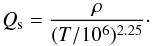 (33)The power 2.25 was used in Eq. (33) because, during the creation of the SAHA-S basic data tables, it leads to the most compact rectangular coverage of the solar model trace (see Fig. 1). At the same time, with that choice, the authors managed to avoid the problematic region of extremely high density which is not relevant to ordinary stars. We note that in future versions of SAHA-S this choice of power might be changed to allow modelling a broader mass range of stars.
The (bijective) transformation above allows us to calculate stellar models with the help of rectangular tables, which is very useful for the necessary interpolations within the tables (see Sect. 5.2). In particular, the choice of a new independent variable Qs instead of ρ makes it possible to interpolate in a two-dimensional, equidistant, and rectangular grid of mesh points. This has the advantage that the two-dimensional mesh can be written as a product of two one-dimensional meshes. In the plane of T−ρ, the SAHA-S mesh points lie inside a parallelogram limited by the blue boundaries in Fig. 1. Compared with the boundaries of the OPAL tables (also plotted in Fig. 1), those of SAHA-S are different because it was specifically developed for solar modeling; however, the table construction of SAHA-S is also necessary for our multi-dimensional non-local spline interpolation, which makes this procedure effective and simple. The track of solar model points is shown by the solid red curve. Solar evolution models can be calculated onward from an early stage of the pre-main sequence, an example of such a calculation is plotted by the dashed red curve.
To assess the possibility of using the SAHA-S tables in its presently available domain to stars of different mass, we have plotted two examples, one for a star with 0.8 M⊙ (orange curve) and the other for a star with 2 M⊙, close to the end of their main sequence lives (magenta curve).
As shown in Fig. 1, we conclude that for low-mass stars, modelling with the SAHA-S EOS is rather limited, whereas for massive main sequence stars it has better prospects. However, for such applications the domain of the tables will have to be expanded toward higher temperatures and lower densities.
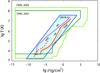 |
Fig. 1 Domain of applicability of the SAHA-S EOS, and two versions of the OPAL EOS. The profiles of main sequence stars with masses 0.8 M⊙, 1.0 M⊙, and 2.0 M⊙ are indicated by the solid orange, red, and magenta curves, respectively. The dashed curve shows the profile of a 1 M⊙ early pre-main sequence model. |
As mentioned above, two additional input parameters of SAHA-S tables are the hydrogen mass fraction X and the heavy-element mass fraction Z. With respect to X, we perform a B-spline interpolation, but in Z our interpolation is linear. We note that the mixture of the heavy elements included in SAHA-S cannot be changed unless a new set of thermodynamic tables is constructed. The current version of SAHA-S EOS includes the eight most abundant elements heavier than helium.
The original SAHA-S thermodynamic quantities provide all the necessary thermodynamic information, but not in the form of the quantities needed by CESAM2k. While SAHA-S provides P, χT, χρ, cV, together with the derivative with respect to the chemical composition (∂P/∂X) | T,ρ, and also the quantities U, (∂U/∂ρ) | T,X, and (∂U/∂X) | T,ρ, CESAM2k requirements include additional quantities that have to be calculated, such as δ, cP, ∇ad, and their derivatives.
5. Bridging between SAHA-S and CESAM2k
To integrate SAHA-S into CESAM2k, we had to apply several modifications. First, a transformation from P(T,ρ) to ρ(P,T) has been performed (see Sect. 5.1). Second, the set of original SAHA-S thermodynamic quantities has been expanded to match the requirements from CESAM2k. The additional quantities are listed in Table 2.
Auxiliary data of SAHA-S.
Third, a B-spline interpolation of the resulting expanded tables has been performed in the variables log (T), log (Qs), and X. The advantage of this type of interpolation is its high efficiency even in three dimensions. Also, it allows the calculation of the derivatives of all tabulated functions and of functions based on the tabulated quantities. Moreover, a B-spline interpolation preserves the smoothness of the thermodynamic functions. Details of the technique are discussed in Sect. 5.2.
Fourth, and finally, we have developed auxiliary routines to provide the transformation from derivatives with respect to Qs to derivatives with respect to ρ, and from derivatives with respect to T, ρ to derivatives with respect to P, T. Our routines use B-spline derivatives with respect to X under constant T and Qs, which are transformed to those at constant P and T (see Sect. 5.3). Previously, in CESAM2k only a finite difference differentiation was used for the latter, requiring extra calls of the EOS procedure.
5.1. Transformation of the EOS to the form ρ(P,T)
When starting from P = P(ρ,T), represented in the form of a set of piece-wise interpolation polynomials of type  (with j being the order), a method to find the inverse functions of these interpolation polynomials (j)S-1(y) is needed. In the linear case (j = 1), the solution of this problem is simple and analytical, but in the case of quadratic and cubic polynomials it results in complicated irrational functions. For cubic splines, an analytical inversion becomes practically useless and numerically inefficient. We therefore solve the inversion problem numerically by the Newton-Raphson iteration method (Press et al. 1992). In particular, for a given P0 we must find the root ρ0 of the equation P0 = P(ρ). The value of the density in step i of the iteration is
 ![Mathematical equation: \begin{equation} \rho ^{(i)} = \rho ^{(i-1)} + \frac{1}{P^\prime (\rho)} \left[ P_0 - P\left(\rho ^{(i - 1)}\right)\right]. \end{equation}](/articles/aa/full_html/2017/10/aa31248-17/aa31248-17-eq134.png) (34)The efficiency of the iterative method strongly depends on the quality of the evaluation of the derivative P′(ρ) during every step of the iteration. In addition to the rather crude but robust method based on finite-difference estimates of the derivative, two other approaches for P′(ρ) are available. The first uses the derivative ∂P/∂ρ |T obtained from the tabulated data of EOS. This method achieves a rapid convergence of the iteration, but it requires an additional interpolation of the quantity χρ(T,ρ,X). The second mathematically more rigorous method consists in obtaining the derivative from the analytical cubic polynomial for P(ρ) with given fixed T,X. In the present paper, we use the method based on interpolation of χρ.
(34)The efficiency of the iterative method strongly depends on the quality of the evaluation of the derivative P′(ρ) during every step of the iteration. In addition to the rather crude but robust method based on finite-difference estimates of the derivative, two other approaches for P′(ρ) are available. The first uses the derivative ∂P/∂ρ |T obtained from the tabulated data of EOS. This method achieves a rapid convergence of the iteration, but it requires an additional interpolation of the quantity χρ(T,ρ,X). The second mathematically more rigorous method consists in obtaining the derivative from the analytical cubic polynomial for P(ρ) with given fixed T,X. In the present paper, we use the method based on interpolation of χρ.
The starting point of the density iteration ρ(0) is a bit tricky, and its choice can affect the convergence rate and number of iterations necessary. Using the inverse linear interpolation function between a pair of mesh points lying nearest to the desired pressure value  for a given value of Tand X, we obtain a reasonably good starting point of the iteration
 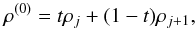 (35)where
 ![Mathematical equation: \hbox{$t = \left[ P - P(\rho _{j + 1}) \right] \left/ \, \left[ P(\rho_j) - P(\rho_{j + 1}) \right]\right.$}](/articles/aa/full_html/2017/10/aa31248-17/aa31248-17-eq143.png) in the interval around P, P(ρj) <P<P(ρj + 1).
in the interval around P, P(ρj) <P<P(ρj + 1).
5.2. Interpolation technique
To represent thermodynamic functions, we use the cubic spline interpolation with special end conditions, known as the not-a-knot condition, following de Boor (1975). Using the de Boor (1978) notation, a cubic spline will have order k = 4.
We interpolate the function f(xi), given on the equidistant mesh xi, i = 1...N, in the interval [a;b]. We use a B-form of the presentation of the splines, where the result is a sum over N basis functions Bj,k(x): 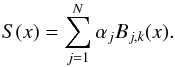 (36)In this representation αj are dependent on f(x), but Bj,k(x) are not. So, to interpolate a number of functions at the same point we need to calculate Bj,k(x) only once. Moreover B-forms can be easily expanded to multi-dimensional interpolation:
 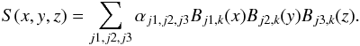 (37)We proceed to calculate basis functions, Bj,k(x), which are used to interpolate to point x.
The definition of Bj,k(x) depends on a mesh of spline-sites tj which is defined not uniquely. Generally, tj may not coincide with any knots of interpolation mesh xj. For the sake of simplicity, we construct t-mesh as follows: 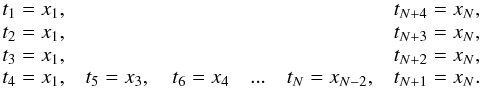 (38)For not-a-knot condition, the first four and the last four knots have multiplicity 4, and the second (i = 2) and penultimate (i = N−1) x-knots are omitted (Fig. 2a). The total number of t-mesh points is N + k.
For a given x, let us define integer index of interval i(x) in t-mesh according to two conditions: ti<ti + 1 and x ∈ [ ti,ti + 1). The first condition in definition of i is important in the case of multiplicative knots. To compute the interpolating polynomial S(x) at the point x within the interval i, only k non-zero basis functions (and corresponding coefficients αi) are needed: 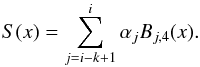 (39)To calculate all needed basis functions at x, it is most efficient to use the recursion relation (de Boor 1978):
 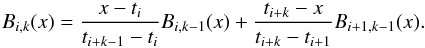 (40)The recursion is started from the first-order spline
  (41)Sometimes Eq. (40) is considered the definition of the basis B-functions.
Figure 2 shows the t-mesh and the B-functions calculated for the interpolation procedure. We note that the B-functions depend on the specific choice of the t-knots.
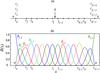 |
Fig. 2 Panel a: Mesh { ti } with not-a-knot end condition; b) cubic B-spline basis functions Bi,k(x). |
Another property of B-splines is the possibility of calculating analytical derivatives of the interpolating polynomials in the form of giving lower order splines. For example, the first derivative (j = 1 in Eq. (12b) de Boor 1978) can be written in the form 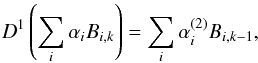 (42)
(42)
where the quadratic splines Bi,k−1 have already been calculated and used in Eq. (40), and where  (43)For all the functions listed in Table 2, files with the appropriate B-spline coefficients for interpolation and differentiation in log T, log Qs, and X, are included in the SAHA-S module.
5.3. Algorithm for calculation of thermodynamic derivatives
To incorporate the SAHA-S EOS into a stellar evolution code, the thermodynamic derivatives with respect to P, T, and X, are needed, as listed in Table 1. The first group is the derivatives of density, and they can be extracted from the terms of Eq. (7):  (44)
(44) (45)
(45) (46)In all these derivatives of density, we have used and δ instead of the basic set of derivatives in Eq. (7). The derivative ∂ρ/∂X|P,T in Eq. (46) is expressed via χX defined by Eq. (6).
Second group of derivatives is of internal energy U: 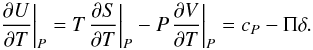 (47)Other symmetrical derivatives can be found in an analogous way:
 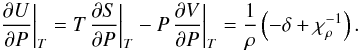 (48)So the corresponding procedure can be simplified and uses only tabulated values cP, χρ, and δ. The last derivative of U with respect to X is expressed via values originally available in SAHA-S table:
 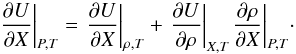 (49)To transform the derivatives from the SAHA-S coordinates of log Qs, log T, and X to the CESAM2k coordinates of P, T, and X, we use
 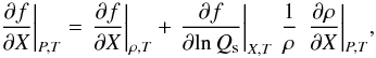 (50)
(50) (51)
(51) (52)where f is any of the quantities from Table 2.
The expression of derivatives with respect to lnQs,lnT through derivatives with respect to lnρ,lnT is given by  (53)
(53) (54)
(54)
6. Comparison of the SAHA-S and OPAL 2001 EOS incorporated in CESAM2k
To demonstrate the correct working of SAHA-S inside CESAM2k, we present the results of computations performed with the stellar evolution code CESAM2k. All figures illustrate the profiles of physical quantities in calibrated models of the Sun. These models differ in the EOS used: OPAL 2001 and SAHA-S, respectively.
The SAHA-S EOS has been incorporated in CESAM2k with the aforementioned interpolation method, which is numerically efficient and, in addition, inside the model it allows interpolation in Z at every point in space and time.
The adiabatic exponent Γ1 of the different models of the present-day Sun is plotted for the deep part of the solar interior (Fig. 3). The outermost part closer to the surface, which would exhibit large variations in Γ1, is not shown. In the deep interior of the convection zone, the difference in Γ1 due to EOS can attain an absolute value up to 10-3. This discrepancy is detectable by present-day helioseismology (Vorontsov et al. 2013). Generally speaking, the discrepancy in Γ1 in Fig. 3 is the result of a difference in the structure of the models. Specifically, a first part of the discrepancy is caused directly by differences in the physical assumptions of the EOS and by a different Z mixture. However, a further change is induced indirectly by those model quantities that depend on the structure variables. The net discrepancy is the sum of these two effects.
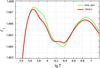 |
Fig. 3 Adiabatic exponent Γ1 in the deeper interior of the Sun (down to the centre). |
The Brunt-Väisälä frequency NBV has significant oscillations in the convection zone if it is computed using Eq. (25), that is, by numerical differentiation of the density. Figure 4 presents the dimensionless value of  computed in models with OPAL 2001 (green curve) and SAHA-S (red curve). The random fluctuations in the case of OPAL 2001 is significantly higher because of higher numerical noise in the OPAL 2001 data tables. The lower level of fluctuations in models with SAHA-S is due to the quality of our spline interpolation and to less numerical noise in the tables. However, even in the case of SAHA-S, the accuracy of numerical differentiation is not sufficient. In particular, repeatedly changes its sign. The situation can be improved by using Eq. (27) in the convection zone (blue curve), which gives a monotonic and negative , as dictated by the physics of a slightly sub-adiabatic stratification.
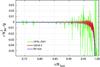 |
Fig. 4 Dimensionless squared Brunt-Väisälä frequency |

The difference in the sound speed between a model with a given EOS on the one hand, and the result of a helioseismic inversion (Vorontsov et al. 2013) on the other hand, is shown in Fig. 5. The red curve refers to a model obtained with the SAHA-S EOS, the green curve to a model with OPAL 2001. The blue curve represents a standard solar model: Model S of Christensen-Dalsgaard et al. (1996), in which an early OPAL version was used (Rogers et al. 1996). This figure shows how sound speed in modern model calculations closely approximates the observational data, and how accurate EOS data should be to enable an adequate analysis. Inside the convection zone, above the location of 0.713r/RSun, the model structure is predominately defined by Γ1, and the differences between the curves reflect the thermodynamic differences between the applied EOS. The required accuracy of the sound speed in EOS calculations has to be better than 10-4 (see Vorontsov et al. 2013, for a detailed analysis).
Most of the difference between the model sound speed below the convection zone is connected to opacities and the general structure of the model core. It is rather difficult to demonstrate specific effects of the EOS here. Common to all solar models is a hump in sound speed just below the bottom of the convection zone. This hump is probably related to the tachocline and overshooting, both of which are poorly treated by current models. The analysis of these model differences is well beyond the scope of the present study.
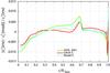 |
Fig. 5 Relative sound-speed-square difference between a helioseismic inversion (Vorontsov et al. 2013) and three different models. |
7. Conclusions
We present the results of the incorporation of the new version of the SAHA-S EOS into an advanced stellar evolution code, CESAM2k. There is a mismatch between the data available in the thermodynamic calculations and the data needed for stellar modelling. These differences are due to the fact that the evolution code calls for quantities as functions of pressure and temperature instead of temperature and density, which are the most common independent variables in thermodynamic computations. The different independent variables require re-writing the set of partial derivatives of the thermodynamic quantities. To avoid time-consuming and noisy finite-difference numerical differentiations during the calculations, throughout we rely on thermodynamic relations and analytic expressions, and on pre-computed values of the auxiliary interpolation coefficients αi. A specific feature of the CESAM2k code is the demand for some extra quantities such as specific heat capacities and adiabatic gradients.
Due to the regular node mesh in the SAHA-S EOS tables, we were able to use an efficient interpolation algorithm in the form of three-dimensional cubic spline functions, allowing us to keepthe smoothness of the functions and their first derivatives, and to provide good estimates of higher partial derivatives, in particular those with respect to chemical composition. With respect to interpolation in Z, we have adopted linear interpolation between adjacent table points.
Our results obtained for the spline coefficients and the necessary interpolation software are available as a freely downloadable FORTRAN module1.
We anticipate that our EOS interface routines can be adapted to other stellar evolution codes.
The SAHA-S EOS has been integrated in the CESAM2k code, and the first results of solar modelling have already been obtained. We have also carried out a preliminary comparison with the results of previous computations which were based on the OPAL EOS.
References
- Baturin, V. A., Ayukov, S. V., Gryaznov, V. K., et al. 2013, in Progress in Physics of the Sun and Stars: A New Era in Helio- and Asteroseismology, eds. H. Shibahashi, & A. E. Lynas-Gray, ASP Conf. Ser., 479, 11 [Google Scholar]
- Chandrasekhar, S. 1939, An introduction to the study of stellar structure (Chicago: The University of Chicago Press) [Google Scholar]
- Christensen-Dalsgaard, J., Däppen, W., Ajukov, S. V., et al. 1996, Science, 272, 1286 [CrossRef] [Google Scholar]
- Cox, J. P., & Giuli, R. T. 1968, Principles of stellar structure(New York: Gordon and Breach) [Google Scholar]
- de Boor, C. 1975, Convergence of cubic spline interpolation with the not-a-knot condition, Tech. Rep., 2876, University of Wisconsin-Madison, Mathematics research center [Google Scholar]
- de Boor, C. 1978, A practical guide to splines (New York: Springer) [Google Scholar]
- Gryaznov, V. K., Ayukov, S. V., Baturin, V. A., et al. 2006, J. Phys. A Math. Gen., 39, 4459 [NASA ADS] [CrossRef] [Google Scholar]
- Gryaznov, V. K., Iosilevskiy, I. L., Fortov, V. E., et al. 2013, Contrib. Plasm. Phys., 53, 392 [NASA ADS] [CrossRef] [Google Scholar]
- Hansen, C. J., & Kawaler, S. D. 1994, Stellar Interiors, Physical Principles, Structure, and Evolution, Astronomy and Astrophysics Library, XIII (Berlin Heidelberg, New York: Springer-Verlag), 445 [Google Scholar]
- Lang, K. R. 1974, Astrophysical formulae: A compendium for the physicist and astrophysicist (New York: Springer-Verlag New York, Inc.), 760 [Google Scholar]
- Mihalas, D., Däppen, W., & Hummer, D. G. 1988, ApJ, 331, 815 [NASA ADS] [CrossRef] [Google Scholar]
- Morel, P., & Lebreton, Y. 2008, Ap&SS, 316, 61 [NASA ADS] [CrossRef] [MathSciNet] [Google Scholar]
- Morel, P., Provost, J., & Berthomieu, G. 1997, A&A, 327, 349 [NASA ADS] [Google Scholar]
- Press, W. H., Teukolsky, S. A., Vetterling, W. T., & Flannery, B. P. 1992, Numerical recipes in FORTRAN, The art of scientific computing, 2nd edn. (Cambridge: Cambridge University Press) [Google Scholar]
- Rogers, F. J., & Nayfonov, A. 2002, ApJ, 576, 1064 [Google Scholar]
- Rogers, F. J., Swenson, F. J., & Iglesias, C. A. 1996, ApJ, 456, 902 [NASA ADS] [CrossRef] [Google Scholar]
- Unno, W., Osaki, Y., Ando, H., Saio, H., & Shibahashi, H. 1989, Nonradial oscillations of stars, 2nd edn. (Tokyo: University of Tokyo Press) [Google Scholar]
- Vorontsov, S. V., Baturin, V. A., Ayukov, S. V., & Gryaznov, V. K. 2013, MNRAS, 430, 1636 [NASA ADS] [CrossRef] [Google Scholar]
- Weiss, A., Hillebrandt, W., Thomas, H.-C., & Ritter, H. 2004, Cox and Giuli’s Principles of Stellar Structure (Cambridge: Cambridge Scientific Publishers Ltd.) [Google Scholar]
All Tables
All Figures
|
Fig. 1 Domain of applicability of the SAHA-S EOS, and two versions of the OPAL EOS. The profiles of main sequence stars with masses 0.8 M⊙, 1.0 M⊙, and 2.0 M⊙ are indicated by the solid orange, red, and magenta curves, respectively. The dashed curve shows the profile of a 1 M⊙ early pre-main sequence model. |
| In the text | |
|
Fig. 2 Panel a: Mesh { ti } with not-a-knot end condition; b) cubic B-spline basis functions Bi,k(x). |
| In the text | |
|
Fig. 3 Adiabatic exponent Γ1 in the deeper interior of the Sun (down to the centre). |
| In the text | |
|
Fig. 4 Dimensionless squared Brunt-Väisälä frequency |
| In the text | |
|
Fig. 5 Relative sound-speed-square difference between a helioseismic inversion (Vorontsov et al. 2013) and three different models. |
| In the text | |
Current usage metrics show cumulative count of Article Views (full-text article views including HTML views, PDF and ePub downloads, according to the available data) and Abstracts Views on Vision4Press platform.
Data correspond to usage on the plateform after 2015. The current usage metrics is available 48-96 hours after online publication and is updated daily on week days.
Initial download of the metrics may take a while.