| Issue |
A&A
Volume 606, October 2017
|
|
|---|---|---|
| Article Number | A79 | |
| Number of page(s) | 12 | |
| Section | Planets and planetary systems | |
| DOI | https://doi.org/10.1051/0004-6361/201730916 | |
| Published online | 16 October 2017 | |
Addressing the statistical mechanics of planet orbits in the solar system
Institut d’Astrophysique de Paris, 98bis bd Arago, 75014 Paris, France
e-mail: This email address is being protected from spambots. You need JavaScript enabled to view it.
Received: 3 April 2017
Accepted: 26 June 2017
Abstract
The chaotic nature of planet dynamics in the solar system suggests the relevance of a statistical approach to planetary orbits. In such a statistical description, the time-dependent position and velocity of the planets are replaced by the probability density function (PDF) of their orbital elements. It is natural to set up this kind of approach in the framework of statistical mechanics. In the present paper, I focus on the collisionless excitation of eccentricities and inclinations via gravitational interactions in a planetary system. The future planet trajectories in the solar system constitute the prototype of this kind of dynamics. I thus address the statistical mechanics of the solar system planet orbits and try to reproduce the PDFs numerically constructed by Laskar (2008, Icarus, 196, 1). I show that the microcanonical ensemble of the Laplace-Lagrange theory accurately reproduces the statistics of the giant planet orbits. To model the inner planets I then investigate the ansatz of equiprobability in the phase space constrained by the secular integrals of motion. The eccentricity and inclination PDFs of Earth and Venus are reproduced with no free parameters. Within the limitations of a stationary model, the predictions also show a reasonable agreement with Mars PDFs and that of Mercury inclination. The eccentricity of Mercury demands in contrast a deeper analysis. I finally revisit the random walk approach of Laskar to the time dependence of the inner planet PDFs. Such a statistical theory could be combined with direct numerical simulations of planet trajectories in the context of planet formation, which is likely to be a chaotic process.
Key words: planets and satellites: dynamical evolution and stability / chaos / celestial mechanics
Sorbonne Universités, UPMC Paris 6 & CNRS, UMR 7095.
© ESO, 2017
1. Introduction
The chaotic dynamics of solar system planets (Laskar 1989; Sussman & Wisdom 1992) raises the question of a statistical approach to planetary orbits. When chaos is significant, a single integration of the equations of motion is not representative of the entire possible dynamics. A description based on the probability density function (PDF) of the planet orbital elements, instead of their time-dependent position and velocity, is essentially more suitable. Such a statistical approach could be combined with usual direct numerical integrations, especially in the context of planet formation, which is likely to be a chaotic process (e.g. Laskar 1997; Malhotra 1999; Hoffmann et al. 2017).
The role of statistical mechanics in assessing the PDF of the planet orbital elements naturally emerges. Recently, the statistical mechanics of terrestrial planet formation has been addressed by Tremaine (2015). In the spirit of a packed planetary systems hypothesis (Fang & Margot 2013), he advances the equiprobability of phase-space configurations verifying a certain criterion for the long-term stability of planetary systems. Within the limitations of the sheared-sheet approximation and the restriction to the planar case, this ansatz permits the analytical computation of any property derivable from the complete N-planet distribution function, such as the distributions of planet eccentricities and semimajor axis differences. The predictions show an encouraging agreement with N-body simulations and data from the Kepler catalogue, while significant discordances arise in the case of radial-velocity data and solar system planets. The simplicity of Tremaine’s ansatz is fundamental to describe the two main steps of the final giant-impact phase of terrestrial planet formation: the excitation of embryo eccentricities and inclinations through mutual gravitational interactions and the subsequent collisions and mergings. However, one could ask for a more fundamental approach, exploiting for instance the integrals of motion (e.g. Kocsis & Tremaine 2011; Touma & Tremaine 2014; Petrovich & Tremaine 2016), in line with the spirit of equilibrium statistical mechanics (Landau & Lifshitz 1969b). Such an approach can actually be set up by focusing on how eccentricities and inclinations are excited by gravitational interactions in an early, collisionless final phase of terrestrial planet formation and by postponing the analysis of collisions to subsequent treatments. As there is no fundamental physical difference between this problem and that of future planetary trajectories in the solar system (Laskar 1996), the latter can provide a benchmark to any statistical theory of planetary orbits to be applied to exoplanet systems. In the present study I address the problem of setting up the statistical mechanics of planetary trajectories in the solar system.
The statistical mechanics of gravitating systems is notoriously challenging (Padmanabhan 1990). Firstly, the system has to be confined in a box to assure a bounded phase space. Then, the non-extensive nature of gravitational energy, due to the long-range character of Newtonian potential, breaks the equivalence between the microcanonical and canonical ensembles, which is typical of systems like neutral gases and plasmas. The long-range nature of gravity also prevents the existence of a thermodynamic limit. In addition to this, the short-range singularity of the gravitational potential requires one to take into account the specific nature of small-scale interactions to guarantee the existence of microcanonical equilibrium states. Finally, the number N of planets in a typical planetary system, even during the giant-impact phase of its formation process, is limited. Therefore, the N ≫ 1 regime is generally inappropriate and so is the employment of a mean field approach1. As pointed out by Touma & Tremaine (2014) mainly in the context of stellar systems, one effective way to construct the statistical mechanics of orbits in a planetary system is to average the planet motion over its fastest timescale, that is the orbital period. As a result of this averaging procedure, each planet is replaced by a massive ring following its Keplerian orbit, whose linear mass density is inversely proportional to the planet orbital velocity, a so-called Gaussian ring (Gauss 1818; Hill 1882; Touma et al. 2009; Kondratyev 2012). In such a system, the rings interact with each other via secular gravitational interactions. Their eccentricities and inclinations relax via exchange of angular momentum, while their semimajor axes are constant and hence are their Keplerian energies (Rauch & Tremaine 1996). Even if there is no theorem assuring that this secular dynamics approaches the actual planet motion, this approach can nevertheless represent the source of important results (Arnold 1978). Indeed, the first clear indication of a chaotic planetary motion in the solar system came from averaged equations of motion (Laskar 1989). Moreover, by using the same secular dynamics, Laskar (2008, from now on L08) numerically computed the PDFs of eccentricity and inclination of the solar system planets. In the present Paper I address the problem of reproducing these PDFs through a statistical mechanics approach.
The paper is structured as follows. In Sect. 2 I briefly recall how secular planet dynamics can be introduced in its simplest form. Then, in Sect. 3 I describe the PDFs of eccentricity and inclination of the solar system planets calculated numerically in L08. I introduce in Sect. 4 the microcanonical ensemble of the Laplace-Lagrange theory to reproduce the statistics of the giant planet orbits. The ansatz of equiprobability in the phase space constrained by the secular integrals of motion is presented in Sect. 5 for the inner planets. Finally, I revisit in Sect. 6 the random walk ansatz of L08 to account for the time dependence of the inner planet PDFs. I conclude by emphasizing the relevance of a statistical theory of planetary orbits in the context of planet formation.
2. Secular planet dynamics
Using standard notation (e.g. Morbidelli 2002), the Hamiltonian of the N = 8 solar system planets can be written as 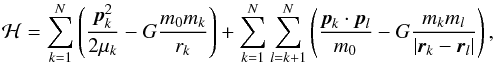 (1)where heliocentric canonical variables rk,pk are employed, m0 is the Sun mass, mk the planet masses, μk = m0mk/ (m0 + mk) the reduced masses, and G the gravitational constant. As usual, the index k lists the planets by increasing semimajor axis, from Mercury to Neptune. The first term on the right side of Eq. (1)is the Hamiltonian of the Keplerian motion, while the second term contains the gravitational interactions among planets. Therefore, it is worthwhile to introduce a set of action-angle variables for the Keplerian motion, e.g. the modified Delaunay variables (Morbidelli 2002), as follows:
 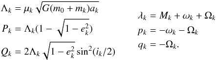 (2)Keplerian orbital elements are used in these definitions: ak is the planet orbit semimajor axis, ek the eccentricity, ik the inclination, Mk the mean anomaly, ωk the argument of perihelion, and Ωk the longitude of node. As long as planets do not experience close encounters and do not lie near mean motion resonances, secular dynamics can be introduced by averaging the Hamiltonian (1)over the fastest motion timescales, i.e. the planet orbital periods. This corresponds to average the Hamiltonian over the mean anomalies Mk,
 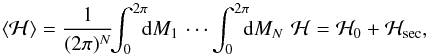 (3)where
  is the total Keplerian energy and
 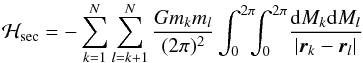 (4)are the orbit-averaged gravitational interactions between planets; the kinetic contribution in the second term on the right side of Eq. (1)averages out to zero over a Keplerian orbit. This averaging procedure corresponds to constructing a secular normal form to first order in planetary masses (e.g. Morbidelli 2002). The action variables Λk are integrals of motion of the secular dynamics (Arnold 1978), and so are the semimajor axes ak. As a consequence, ℋ0 is an additive constant that may be dropped from the Hamiltonian. The single-planet secular phase space is four-dimensional and compact with the canonical volume element given by dpkdqkdPkdQk. The secular contribution of general relativity is of primary importance for the long-term dynamics of the solar system inner planets (e.g. L08). The secular Hamiltonian accounting for the leading relativistic correction is given by
 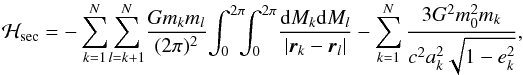 (5)where c is the speed of light. A short derivation of the general relativistic contribution is presented in Appendix A for future reference.
When eccentricities and inclinations are sufficiently small, ek,sin(ik/ 2) ≪ 1, it is valuable to develop the secular Hamiltonian in a power series of these variables. Neglecting terms of the fourth order and smaller, one obtains the Laplace-Lagrange (LL) linear secular theory,  (6)where I have introduced the Poincaré canonical variables at the lowest order in eccentricity2,
 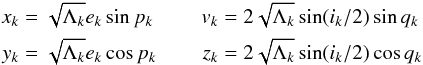 (7)and for instance xT = (x1,...,xN). The elements of the matrices A and B are given in Appendix B. These matrices are real and symmetric and can therefore be diagonalized through orthogonal matrices OA and OB,
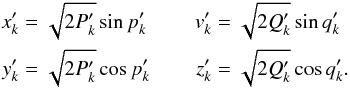
 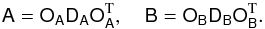 (8)The elements of the diagonal matrices DA and DB are the eigenvalues of A and B, respectively, and the columns of OA and OB are their normalized eigenvectors. New action-angle coordinates P′,Q′,p′,q′ can be introduced by combining the following canonical transformations:
 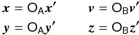 (9)
(9) (10)Employing the new variables, the LL Hamiltonian becomes
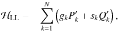 (11)where gk and sk are the eigenvalues of the matrices A and B, respectively. According to the corresponding Hamilton equations, the actions
  and
and  are integrals of motion, while the angles
  and
and  change linearly with time at constant frequencies −gk and −sk, respectively. Therefore, the time dependence of the Poincaré variables xk,yk,vk,zk turns out to be the superposition of N harmonics with different frequencies and amplitudes. In the present study, I refer to each of these harmonics as a LL mode and I follow the conventional ordering of the frequencies gk and sk (Morbidelli 2002, Table 7.1).
Generally speaking, the dynamics of a planetary system obeys the conservation of mechanical energy, momentum, and angular momentum. The secular dynamics verifies the conservation of momentum in the barycentric reference system in a trivial way: as Keplerian orbits are closed, the average of planet momenta over mean anomalies identically vanishes. Therefore, the dynamics resulting from the secular Hamiltonian (5)must conserve energy and angular momentum. This can be easily shown to be the case in LL dynamics (e.g. Kocsis & Tremaine 2011). As formula (11)shows, the LL Hamiltonian is a function of the action variables only. Because these are integrals of motion, the conservation of energy follows. The angular momentum content of a planetary system can be described by the following quantities: 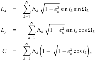 (12)where x,y,z are the Cartesian coordinates related to the definition of the Keplerian elements ik,ωk, and Ωk (Morbidelli 2002)3. The variables Lx and Ly are the components of the angular moment lying on the xy-reference plane, while C is the angular momentum deficit (AMD) (Laskar 1997, 2000), i.e. the difference between the angular momentum that planets would have on coplanar, circular orbits and Lz, the component of the total angular momentum perpendicular to the reference plane. The AMD can be expressed as
 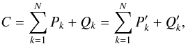 (13)where I have used the definitions (2)and the fact that the matrices OA and OB, appearing in the transformation (9), are orthogonal. As the action variables P′ and Q′ are conserved in LL dynamics, the AMD is also a conserved quantity4. Conservation of Lx and Ly derives from the properties of the matrix B. As shown in Appendix B, one of the eigenvalues sk is zero and
  is, up to a sign, the corresponding normalized eigenvector. By convention (Morbidelli 2002, Table 7.1), the null eigenvalue is chosen to be s5. Moreover, neglecting terms of order three in eccentricities and inclinations, one has
  (14)All this implies that in LL dynamics the following identities are verified:
  (15)where I have used the fact that OB is orthogonal,
  , and its columns are the normalized eigenvectors of B. As the frequency s5 is zero,
  does not change with time. Therefore,
  and
and  are integrals of motion and hence are Lx and Ly.
 |
Fig. 1 Eccentricity and inclination PDFs of the solar system giant planets. The PDFs of L08 are plotted in solid lines, while those predicted by the microcanonical distribution function (16)are shown in dashed lines. The inclinations are computed with respect to the J2000 ecliptic. |
3. Probability density functions of Laskar (2008)
In L08 Laskar performs a statistical analysis of the future planet orbits in the solar system. He employs 1001 integrations of secular equations over the 5 Gyr of the remaining lifetime of the Sun before its red giant phase. These integrations differ for the initial conditions, which are obtained with small variations of the initial Poincaré variables of the VSOP82 solution (Bretagnon 1982). The total integration time is divided in 250 Myr intervals and statistics are performed over each interval recording the state of the 1001 solutions with a 1 kyr time step. Normalized PDFs of planet eccentricities and inclinations are then estimated. The PDFs of the giant planets are plotted in Fig. 1, while in Fig. 2 those of the inner planets are shown. Unfortunately, the data behind the L08 PDFs are not currently available (Laskar, priv. comm.). Therefore, I have extracted these curves from the original plots through WebPlotDigitizer (Rohatgi 2017). This works fine for the giant planets PDFs and the eccentricity PDFs of the inner planets, as Laskar plotted them separately at three different times. Because of chaotic diffusion, such an extraction is infeasible for the inclination PDFs of the inner planets, which Laskar plotted at several different times on the top of each other. In this case I use as a reference Laskar’s fits instead of the original numerical PDFs, even if some differences exists between these curves, especially in the tails.
The dynamics considered by Laskar is more accurate than the dynamics I introduced in Sect. 2, as Laskar’s secular Hamiltonian contains terms of order two in planetary masses and six in eccentricities and inclinations. This is why he conjectures that, even though his PDFs are obtained through secular equation, they should be nevertheless close to those arising from the full, non-averaged, dynamics. While analysing these PDFs, what strikes Laskar is the very different shape between the giant planets curves and those of the inner planets. The PDFs of the outer planets are characterized by two peaks and restricted to a certain range of eccentricities and inclinations. In contrast, those of the inner planets have zero value at e = 0 and i = 0, a single peak and continuous decaying at large eccentricities and inclinations. On the basis of these differences, Laskar takes two different approaches in explaining his numerical PDFs. By means of a frequency analysis applied to the outer planet motion, he shows that the PDF of a quasi-periodic approximation of their dynamics can reproduce the numerical PDFs very accurately. On the other hand, to take into account the significant chaotic diffusion existing in the statistics of the inner planets, Laskar fits their PDFs through a Rice distribution (Rice 1945). Indeed, he assumes that, because of chaotic diffusion, the Poincaré variables (7)become practically independently Gaussian distributed over long timescales, with a non-zero mean and a variance that increases linearly with time, as in a diffusion process.
 |
Fig. 2 Eccentricity and inclination PDFs of the solar system inner planets. The PDFs of L08 are plotted in solid lines at three different times, t = 500 Myr, 2.5 Gyr, and 5 Gyr, to illustrate chaotic diffusion (the PDF broadens and its peak decreases as time increases; the inclination PDFs are not the original PDFs, but the Rice distributions fitted by Laskar, see Sect. 3 for explanations). The PDFs predicted by the microcanonical ensemble of the Laplace-Lagrange theory, Eq. (16), are shown in dashed line. The inclinations are computed with respect to the J2000 ecliptic. |
4. Giant planets
According to secular dynamics, the orbital motion of the giant planets is well approximated by a quasi-periodic time function (L08). Indeed, chaotic diffusion is very limited for the outer planets; their PDFs virtually do not change with time. A certain chaotic behaviour arises from the full equations of motion (Sussman & Wisdom 1992), but according to L08 this is irrelevant to the overall structure of the PDFs. Taking advantage of this regularity of the giant planets, it is straightforward to predict the PDF of their Keplerian orbital elements. Neglecting chaotic diffusion, the most basic quasi-periodic dynamics is that resulting from the LL Hamiltonian, Eq. (11). Such a motion is ergodic and the asymptotic stationary probability density is given by the microcanonical ensemble (Arnold 1978). It is straightforward to write down the corresponding PDF employing the integrals of motion (Landau & Lifshitz 1969b),  (16)where δ stands for the Dirac delta and the bar indicates the initial value of the corresponding variable5. This PDF reflects the conservation of the action variables P′,Q′ in the LL dynamics, while the angle variables are uniformly distributed over the (2N−1)-dimensional torus T2N−1; the angle is conserved because the angular momentum is conserved (see Sect. 2). The following integral formula for the PDFs of eccentricity and inclination can be obtained (Mardia 1972):
 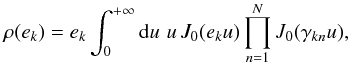 (17)where J0 is the Bessel function of the first kind and order zero and
  . A similar formula holds for the inclination ik. Otherwise, these PDFs can be very rapidly estimated by direct sampling of Eq. (16)and using transformations (10), (9), and (7). The distribution function (16)is time independent and describes the statistics of planet orbits over timescales much longer than the timescale of the LL dynamics (dozens of kyr to few Myr for the solar system planets). Since the PDFs of Laskar are constructed over 250-Myr intervals, one can expect the statistics of the giant planets resulting from Eq. (16)to agree with that of L08. Therefore, I plot in Fig. 1 the PDFs predicted by the microcanonical distribution (16), along with the PDFs found by Laskar. The agreement between the two curves is indeed very satisfactory for the inclination PDFs, with a very good match for Jupiter and Saturn and minor differences in the case of Uranus and Neptune. The agreement is also good for the eccentricity PDFs of Jupiter and Saturn, while some major discordances arise in the eccentricity PDFs of Uranus and Neptune. Even though the shape of the PDFs is correctly reproduced by the microcanonical density (16)in both cases, the endpoints of the eccentricity interval over which the PDFs vary are somewhat different from L08. However, the reason for such a discrepancy is clear. The LL Hamiltonian (11)employed to derive the microcanonical distribution (16)is valid up to the third order in eccentricities and inclinations. This regime is meaningful for the giant planets of the solar system, whose eccentricities and inclinations are small. However, the terms of the fourth order in e and i in the Hamiltonian (5)yield non-linearities in the corresponding Hamilton equations and produce higher order harmonics in the eccentricity and inclination time dependence6. The amplitude of these additional harmonics is generally much smaller than that of the LL modes, but some of the higher order harmonics can nevertheless contribute to a significant level. Bretagnon (1974, Tables 12 and 13) reports the amplitudes of these higher order harmonics. From the Bretagnon tables it is clear that their contribution is bigger for eccentricities than inclinations and for Uranus and Neptune than for Jupiter and Saturn. This is in agreement with Fig. 1. Moreover, the amplitudes of the higher order harmonics are roughly in accord with the size of the discrepancies in Fig. 1. Generally speaking, the agreement between the predictions of the microcanonical distribution (16)and the PDFs found by Laskar is very satisfactory when one realizes the simplicity of the LL approximation. Moreover, a better agreement can be obtained extending the analysis of Sect. 2 to higher order terms in eccentricities, inclinations, and masses. In principle, this could be carried out by means of a perturbation approach to the Hamiltonian (1)based on successive quasi-identity canonical transformations and normal forms (Morbidelli 2002)7.
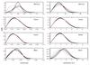 |
Fig. 3 Eccentricity and inclination PDFs of the solar system inner planets. The same as Fig. 2, except that the dashed lines represent here the predictions of the ansatz (18). |
5. Inner planets
The analysis of the giant planet orbits is based on the assumption that the effect of chaos on their motion is largely negligible. This is not the case for the inner planets. Laskar (1994) already showed that the orbits of Mercury and Mars are affected by a significant chaotic diffusion over 5 Gyr, while this diffusion is moderate for Venus and the Earth. A first interesting step in analysing the structure of the PDFs found by Laskar in case of inner planets is to consider what the distribution function (16)predicts for their eccentricities and inclinations. This is illustrated in Fig. 2, where I also plot the corresponding L08 PDFs at three different times, t = 500 Myr, 2.5 Gyr, and 5 Gyr, to illustrate chaotic diffusion. As one might expect, there is no general agreement between the two curves. Nevertheless, it is interesting to note that, contrary to what could emerge from the analysis by Laskar in L08, the difference in shape between the giant and inner planet PDFs is not fundamental. Figure 2 shows that Eq. (16)based on LL dynamics is a priori able to produce the general shape of the inner planet PDFs, i.e. the zero value and positive linear slope at e = 0 and i = 0, and the continuous decaying at large eccentricities and inclinations. This is particularly evident in the Venus and Earth eccentricity curves and is due to the strong linear coupling existing between several LL modes in the Earth and Venus dynamics. Analogue strong couplings are not present in the LL dynamics of the giant planets. This explains the different shape of their PDFs with two peaks and a zero probability outside a certain range (Fig. 1). This is also the case for Mercury, which justifies the strong differences between the corresponding PDFs found by Laskar and Eq. (16)in Fig. 2.
Since the effect of chaos is relevant for the long-term dynamics of the inner planets, I searched for a more pertinent statistical description than one based on quasi-periodic motion. The chaotic nature of planet dynamics allows for sharing of angular momentum between the action variables, which would otherwise be constant. This chaotic diffusion of angular momentum is already mentioned in Laskar (1996) and has been recently illustrated in Wu & Lithwick (2011). The simplest statistical approach is to assume that, by consequence, the motion of the inner planets uniformly visits the subset of the phase space defined by the conservation of angular momentum L and energy ℋsec. Clearly, the fact that chaotic diffusion finally leads to such a uniform phase-space measure cannot be strictly true over 5 Gyr, as the time dependence of the inner planet PDFs is still evident at that time. More probably, a uniform exploration could indeed occur adiabatically on a smaller subset of the phase space than that allowed by the conservation of angular momentum and energy only. Such a domain could be in principle determined by studying the higher order terms in the Hamiltonian (5). The hypothesis of equiprobability in the phase space is the best estimate that one can make without a deeper analysis of the dynamics (Jaynes 1957). It is also so simple that it is worthwhile to investigate its predictions before undertaking more involved studies. Indeed, the idea of equipartition between LL modes has already been considered from a dynamical perspective by Wu & Lithwick (2011). Moreover, even though it leads to a stationary distribution function, such an ansatz seems nevertheless appropriate to the Earth and Venus, since their PDFs diffuse very slowly over time and can be still useful to understand the main factors contributing to the overall structure of Mercury and Mars PDFs.
Partition of the current AMD in the solar system.
Since the giant planets are well described by the microcanonical distribution (16), in which all the LL action variables are fixed, it is clear that an equiprobability simply based on conservation of the total angular momentum and energy of all the planets would not produce reasonable results. To achieve a global description of giant and inner planets at once, one needs to statistically disconnect them. To this end, it turns out that the total angular momentum of the inner planets is fairly independent of that of the giant planets. More precisely, Laskar (1997) has shown that the flux of AMD from the large reservoir of the outer planets to the inner planets is moderate over 5 Gyr. As a first approximation, one can therefore assume that the total AMD of the inner planets is constant. Moreover, from Eq. (13)one can interpret the action variables and as the AMD content in the corresponding LL mode. These considerations suggest fixing the action variables corresponding to the modes k ∈ { 5,6,7,8 }, as these are the only modes that are relevant for the dynamics of the outer planets8. Indeed, with this choice the conservation of the total AMD reduces to that of the quantity  , whose initial value is very close to the initial total AMD of the inner planets, as shown in Table 1. The remaining action variables, corresponding to the modes k ∈ { 1,2,3,4 }, can then be allowed to vary stochastically according to equiprobability. The statistics of the giant planet orbits would therefore be virtually identical to that shown in Fig. 1.
Among the integrals of motion, the AMD is of particular interest. For instance, Laskar (1997, 2000) has highlighted its role in the orbital configuration of planetary systems. An important reason for this relevance is that, contrary to Eqs. (11)and (14), the simple Eq. (13)is valid to all orders in eccentricities and inclinations. I then start to investigate the predictions of equiprobability based on AMD conservation only. Conservation of energy is added later. The ansatz corresponding to the above considerations is written 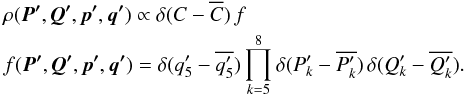 (18)Conservation of Lx and Ly to second order in eccentricities and inclinations is contained in this distribution function as the variables
  and are set to their initial values (see Eq. (15)). I do not have a simple analytical formula for the PDFs of eccentricity and inclination. However, they can be calculated numerically very rapidly by direct sampling, as illustrated in Appendix D. Moreover, I present an analytical characterization of these PDFs in Appendix C. The predictions of the ansatz (18)are compared in Fig. 3 with the PDFs found by Laskar. The probability density (18)reproduces Venus and Earth PDFs very satisfactorily. A detailed comparison in the case of Earth is shown in Figs. 4 and 5. The agreement is remarkable if one considers the simplicity of the ansatz and that it does not contain any free parameter9. For what concerns the PDFs of Mars and that of the inclination of Mercury, the predictions are still reasonable as the differences with the numerical PDFs are of the same order of magnitude of the PDF diffusion over time. Indeed, in these cases one could a priori interpret the predicted curves as the long-term, stationary limit of the PDFs found by Laskar. However, this interpretation breaks down when one considers the eccentricity PDF of Mercury, as shown in detail in Fig. 6. In this case, the predicted PDF is substantially different from the numerical PDFs. In particular, the mean of the curves found by Laskar is not correctly reproduced by the ansatz. It is clear that equiprobability, as applied in Eq. (18), is far to approximate the actual Mercury dynamics.
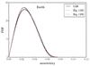 |
Fig. 4 Eccentricity PDF of the Earth. The same as Fig. 3 with the addition of the prediction of Eq. (19)in dash-dotted line. |
One can add to the ansatz (18) the conservation of secular energy at quadratic order in eccentricities and inclinations (see Eq. (11)),  (19)In Appendix D, I suggest an algorithm to efficiently sampling this distribution function. The addition of energy conservation does not change in a substantial way the predictions shown in Fig. 3. The principal consequence is that the average AMD in a single LL mode depends now, for k ≤ 4, on the mode considered via the specific values of the frequencies gk and sk. In contrast, Eq. (18)predicts an average AMD independent of the particular mode (see Appendix C). This slightly shifts the predicted PDFs, without changing the validity of the above considerations. This is shown in the case of Earth in Figs. 4 and 5, and in Fig. 6 for Mercury.
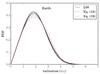 |
Fig. 5 Inclination PDF of the Earth. The same as Fig. 3 with the addition of the prediction of Eq. (19)in dash-dotted line. |
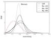 |
Fig. 6 Eccentricity PDF of Mercury. The same as Fig. 3 with the addition of the predictions of Eq. (19)in dash-dotted line and Eq. (20)in dotted line. |
The major disagreement between the predictions of equiprobability in the phase space and the curves of Laskar occurs for the eccentricity of Mercury, which is the less massive planet and has the highest typical eccentricity and inclination10. As suggested above, a kind of equiprobability ansatz could still be valuable if applied to a more restricted phase-space domain than that defined by the conservation of the total inner planet AMD and energy. If, as a matter of speculation, one restricts the equiprobability domain by setting the action variable  to its initial value, i.e.
  (20)the predicted PDF of Mercury eccentricity starts to reproduce the characteristic mean value of the corresponding curves of Laskar, as shown in Fig. 6. This is related to the fact that the chaotic dynamics of Mercury eccentricity keeps a clear memory of the dominant LL mode 11. However, it is clear that more involved analyses, taking into account higher order terms in the Hamiltonian (5), are needed to reproduce the numerical PDFs closely.
6. Random walk approach to chaotic diffusion
Reproducing the PDFs of the inner planets is particularly difficult because of the time dependence of these curves. The complexity of describing diffusion of the integrals of motion in weakly non-linear systems, starting from a given partition between linear modes, is perhaps best illustrated by the famous Fermi-Pasta-Ulam-Tsingou problem (Fermi et al. 1955). As stated in Sect. 3, in L08 the inner planet PDFs are fitted by means of a Rice distribution (Rice 1945), whose parameters depend on time to account for the curve diffusion. Laskar justifies the choice of this particular distribution by stating that, because of chaotic diffusion, Poincaré variables (7)could behave similar to independent Gaussian random variables over a long timescale. In what follows I try, in the simplest way, to frame this ansatz in the context of the present paper, showing the difficulties of such a random walk approach.
In the following discussion I focus on the degrees of freedom related to eccentricity, but a similar analysis applies to the inclination degrees of freedom. According to the microcanonical distribution function (16), the PDF of the rectangular variable hk = eksin(pk) (i.e. marginalized over the remaining Poincaré variables) can be shown to be12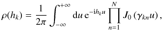 (21)where
  is the imaginary unit, J0 the Bessel function of the first kind and order zero, and . Depending on the coefficients γkn, the PDF (21)can be double-peaked and strongly different from a Gaussian distribution. Moreover, since ρ(−hk) = ρ(hk), the mean value of hk is zero. It seems doubtful whether chaotic diffusion, acting on the LL modes, can drive Poincaré variables to the Gaussianity suggested by Laskar. Therefore, I set up the random walk approach on a slight different basis. On a secular timescale tsec of few Myr, the motion of the inner planets is well reproduced by a quasi-periodic time function. On a Lyapunov timescale, tLyap ≃ 5 Myr, chaos starts to decorrelate the actual motion from the initial quasi-periodic approximation. On a much more longer timescale, t ≫ tLyap, the precise nature of the chaotic terms in the Hamiltonian (5)is possibly irrelevant in assessing the general form of the inner planet PDFs. Considering such a case, I propose an ansatz in which the stochastic dynamics of the Poincaré variables
  and
and  is given by the following superposition of a secular term and a chaotic term:
  (22)where
  13. The stationary random variable rsec describes the statistics of the LL dynamics and corresponds to the microcanonical ensemble (16),
 ![Mathematical equation: \begin{equation} \label{eq:LL_pdf} \rho_{\mathrm{sec}}(x'_k, y'_k) = \frac{\delta \left[ r_k - \left(2 \overline{P'_k} \right)^{1/2} \right]}{2 \pi \left(2 \overline{P'_k} \right)^{1/2}} , \end{equation}](/articles/aa/full_html/2017/10/aa30916-17/aa30916-17-eq112.png) (23)where
(23)where  . The time-dependent chaotic component is modelled by the following Langevin equation:
  (24)where η is a white noise, i.e.
  (25)for all times t,t′ ≥ 0. For simplicity I have assumed an isotropic diffusion in the phase space of the LL mode k. The diffusion coefficient Dk is a free parameter in this model. Moreover, I choose the initial condition on the chaotic term to match the LL dynamics,
  (26)Since the random variables rsec and rchaos are independent, the PDF of r is given by the convolution of the PDF of rsec, ρsec, with that of rchaos, ρchaos. Therefore one has
  (27)The PDF of the random variable satisfying Eqs. (24)–(26)is the Green function of the Fokker-Planck equation
 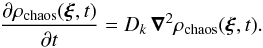 (28)This Green function is
 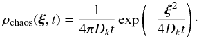 (29)Substituting Eqs. (23)and (29)in Eq. (27)one gets
 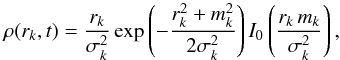 (30)where I0 indicates the modified Bessel function of the first kind and order zero,
  and
and  . Therefore, one obtains a Rice distribution for the variable
  . In the case where the variables xk and yk are dominated by one particular LL mode, i.e. | γkl | ≫ | γkn | for a certain index l and for all n ≠ l, the PDF of the eccentricity ek turns out to be a Rice distribution with parameters
 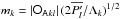 and
and 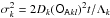 . In this limiting case one thus recovers Laskar’s ansatz. This is because the Rice distribution describes the envelope of a sine wave plus Gaussian noise (Rice 1945), as already mentioned in L08. However, within the present framework, mk is not a free parameter as in L08, but it is set up by the initial LL dynamics. I compare in Table 2 the value of mk given in L08 (Table 6) for the eccentricity PDFs to the prediction of Eq. (30)when one considers for each planet only the LL mode with the biggest amplitude. The physical meaning of the parameter mk clearly emerges in the present framework.
Parameter mk of a Rice distribution reproducing the PDF of the eccentricity of the inner planets.
As shown in Table 2, the PDF (30)casts some light on the fits of Laskar in L08. Nevertheless, it cannot reproduce the numerical PDFs accurately, even if the diffusion coefficients Dk are free parameters. There are a couple of reasons for that. Firstly, the initial distribution (23)is based on the LL dynamics. However, terms of higher order in eccentricities and inclinations in the Hamiltonian (5)are of primary importance for the inner planets. To have a faithful representation of their initial quasi-periodic dynamics one has to go beyond the LL approximation. The other principal limitation of the present framework is that PDF (30)cannot reproduce the slightly decreasing peak positions of Mars PDFs. Indeed, one has  , which means that the average content of AMD in the LL mode k is an increasing function of time. Therefore, the PDFs of eccentricity and inclination can only diffuse towards increasing mean values of the corresponding random variable. The reason for this behaviour is that the random walk considered above does not take into account either the conservation of AMD or that of energy. Indeed, if one assumes that the AMD of the inner planets is conserved over time, it is understandable that Mercury, Earth, and Venus PDFs diffuse towards increasing mean values, while Mars PDFs diffuse towards decreasing values. Therefore, it would be a considerable improvement to set up a random walk exploiting the secular integrals of motion. Such a modification would end in a feedback dynamics between rsec and rchaos in Eq. (22).
7. Conclusions
Motivated by the chaotic dynamics of solar system planets and the stochastic nature of planet formation, I address in the present paper the construction of a statistical description of planetary orbits. I suggest that such an approach can be based on the statistical mechanics of secular dynamics. Considering the solar system as a benchmark, I try to reproduce the PDFs of eccentricity and inclination calculated numerically by Laskar (2008). I show that the statistics of the giant planet orbits is well reproduced by the microcanonical ensemble of the Laplace-Lagrange linear secular dynamics. This is particularly relevant as such a theory can be directly applied to a generic planetary system. Minor discrepancies in this description are connected to higher-than-quadratic terms in the planet Hamiltonian. Their contribution could be taken into account by improving the perturbation approach via successive quasi-identity canonical transformation and normal forms. I then try to reproduce the statistics of the inner planet orbits through the ansatz of equiprobability in the phase space constrained by the secular integrals of motion, namely angular momentum and energy. Within the limitations of a stationary model, such an ansatz allows one to easily and accurately reproduce the structure of Venus and Earth PDFs without any free parameter. However, major discrepancies rise in the case of Mercury eccentricity. I finally show the difficulties of constructing a random walk to model the chaotic diffusion of the inner planet PDFs, following the original ansatz of Laskar (2008). Within certain limitations, the PDF I obtain allows one to illustrate the physical meaning of one of the free parameters in Laskar’s ansatz.
It is clear that the above description of the inner planet statistics has to be improved. One has to taken into account higher-than-quadratic terms in the planet Hamiltonian. Generally speaking, one could think of using the full expression of the secular energy, following Eq. (5). The problem would then be how to sample the corresponding microcanonical ensemble in an efficient way. Another viable approach could be to start constructing an ad hoc model for Mercury, since it shows the most relevant discrepancies with respect to the proposed ansatz. Such an approach could consist in considering Mercury as a test particle in the gravitational field of the other solar system planets, whose orbits are fixed (Boué et al. 2012; Batygin et al. 2015). With a selection of the most important higher order terms relevant for the non-linear dynamics of Mercury, important improvements could be achieved in reproducing the PDFs of its eccentricity and inclination. With respect to the random walk approach presented in Sect. 6, a considerable improvement would be taking into account the conservation of angular momentum deficit and energy. Even if such a model is not completely predictive, as the diffusion in the phase space is described by free parameters, it could be nevertheless really instructive in judging how the conservation of the integrals of motion constrains the relaxation of the Laplace-Lagrange action variables.
The relevance of a statistical description of planet orbits in a generic planetary system is particularly manifest if one considers the model of planet spacing by Laskar (2000; see also Laskar & Petit 2017). In this approach to planet formation, Laskar describes the collisionless dynamics of planetary embryos by a stochastic variation in their orbital elements that conserves the total angular momentum deficit. Conservation of mass and linear momentum is taken into account to model the result of collisions, during which the total angular momentum deficit decreases. Collisions stop when the total angular momentum deficit is too small to allow for further closeencounters. With these simple assumptions, Laskar is able to show how the structure of a generic planetary system derives from the initial mass distribution of planetary embryos. As already pointed out by Tremaine (2015), the Laskar model is not unique because it requires an ad hoc prescription for the random evolution of the orbital elements between collisions. Statistical descriptions, such as those in Sects. 4 and 5 of this paper, can provide such a prescription on the basis of solid physical arguments. A statistical approach to planetary orbits could then be useful in studying planet formation, in combination with standard N-body simulation of planetary trajectories. Evidently, collisions have to be taken into account when addressing planet formation, while they are negligible for the future 5 Gyr of the solar system as long as one is concerned with the bulk of the planet PDFs. Finally, such a statistical theory would be even more pertinent to asteroids because of their large number. Moreover, the eccentricity distribution in the main asteroid belt (Malhotra & Wang 2017) seems to share similarities with the inner planet PDFs treated in this study. This should constitute the subject of future studies.
The lack of the N → + ∞ limit might seem to question the usefulness of employing statistical mechanics. Actually, the foundation for such an approach relies on the chaotic nature of planet dynamics and not on their number N.
Throughout this paper, by Poincaré variables I mean their limiting form at low eccentricity.
The xy-reference plane is typically chosen to be perpendicular to the total angular momentum vector. However, in this study the ecliptic plane is the reference plane, since this is the choice made in L08.
The conservation of AMD holds at all orders in secular dynamics and is not restricted to the LL approximation (e.g. Laskar & Petit 2017).
In the present study these initial values are chosen to match the initial conditions of the VSOP82 solution (Bretagnon 1982, Tables 4 and 5), which are employed in L08.
These higher order terms also affect amplitude and frequency of the LL modes. The secular Hamiltonian (5)is itself valid to the first order in planetary masses. Contributions from higher order terms in mk adjust the amplitude and frequency of the harmonics.
Obviously, one does not mean by that a fully convergent perturbation series, but only to take into account the main non-linear harmonics in a Hamiltonian framework.
As stated in Sect. 2, I adopt the conventional ordering of the LL modes (Morbidelli 2002, Table 7.1).
To fit his PDFs Laskar employs three free parameters for each planet and each orbital element (eccentricity or inclination).
As Boué et al. (2012) and Batygin et al. (2015) show, the dynamics of Mercury treated as a test particle in the gravitational field of the other planets, whose orbits are fixed, can be described by a time-independent Hamiltonian, which is therefore an integral of motion and maintains some memory of the initial conditions.
This results immediately from the following facts: the characteristic function of sin(ω), with ω uniformly distributed over [0,2π], is the Bessel function of the first kind and order zero; the characteristic function of the sum of independent random variables is the product of the corresponding characteristic functions.
Since the action variables P′ are conserved in the LL dynamics, it is reasonable to consider them as a starting point. However, as the boundary condition  applies, the most simple and straightforward approach is to use Poincaré variables and , which are defined on the entire real line.
Acknowledgments
I am grateful to the two anonymous referees for their careful reading of the paper and the very pertinent points. I also acknowledge the fruitful discussions with A. Morbidelli, J. Touma, J. Laskar, J. Teyssandier, N. Cornuault, and L. Pittau. I finally thank J.-P. Beaulieu for his support and help in reviewing the manuscript.
References
- Arnold, V. I. 1978, Mathematical Methods of Classical Mechanics (New York: Springer) [Google Scholar]
- Batygin, K., Morbidelli, A., & Holman, M. J. 2015, ApJ, 799, 120 [NASA ADS] [CrossRef] [Google Scholar]
- Boué, G., Laskar, J., & Farago, F. 2012, A&A, 548, A43 [NASA ADS] [CrossRef] [EDP Sciences] [Google Scholar]
- Bretagnon, P. 1974, A&A, 30, 141 [NASA ADS] [Google Scholar]
- Bretagnon, P. 1982, A&A, 114, 278 [NASA ADS] [Google Scholar]
- Fang, J., & Margot, J.-L. 2013, ApJ, 767, 115 [NASA ADS] [CrossRef] [Google Scholar]
- Fermi, E., Pasta, J., & Ulam, S. 1955, Studies of non-linear problems, Tech. Rep., Document LA-1940 [Google Scholar]
- Gauss, C. F. 1818, Determinatio Attrationis Quam in Punctum Quodvis Positionis (Gottingen: Heinrich Dieterich) [Google Scholar]
- Hill, G. W. 1882, US Nautical Almanac Office Astronomical paper, 1, 315 [Google Scholar]
- Hoffmann, V., Grimm, S. L., Moore, B., & Stadel, J. 2017, MNRAS, 465, 2170 [NASA ADS] [CrossRef] [Google Scholar]
- Jaynes, E. T. 1957, Phys. Rev., 106, 620 [Google Scholar]
- Kocsis, B., & Tremaine, S. 2011, MNRAS, 412, 187 [NASA ADS] [CrossRef] [Google Scholar]
- Kondratyev, B. P. 2012, Sol. Syst. Res., 46, 352 [NASA ADS] [CrossRef] [Google Scholar]
- Landau, L. D., & Lifshitz, E. M. 1969a, Mechanics (Oxford: Pergamon Press) [Google Scholar]
- Landau, L. D., & Lifshitz, E. M. 1969b, Statistical Physics, Pt. 1 (Oxford: Pergamon Press) [Google Scholar]
- Landau, L. D., & Lifshitz, E. M. 1975, The Classical Theory of Fields (Oxford: Pergamon Press) [Google Scholar]
- Laskar, J. 1989, Nature, 338, 237 [NASA ADS] [CrossRef] [Google Scholar]
- Laskar, J. 1994, A&A, 287, L9 [NASA ADS] [Google Scholar]
- Laskar, J. 1996, in Dynamics, Ephemerides, IAU Symp., 172, 75 [NASA ADS] [Google Scholar]
- Laskar, J. 1997, A&A, 317, L75 [NASA ADS] [Google Scholar]
- Laskar, J. 2000, Phys. Rev. Lett., 84, 3240 [NASA ADS] [CrossRef] [PubMed] [Google Scholar]
- Laskar, J. 2008, Icarus, 196, 1 [NASA ADS] [CrossRef] [Google Scholar]
- Laskar, J., & Petit, A. 2017, A&A, 605, A72 [NASA ADS] [CrossRef] [EDP Sciences] [Google Scholar]
- Malhotra, R. 1999, Nature, 402, 599 [NASA ADS] [CrossRef] [Google Scholar]
- Malhotra, R., & Wang, X. 2017, MNRAS, 465, 4381 [NASA ADS] [CrossRef] [Google Scholar]
- Mardia, K. V. 1972, Statistics of Directional Data (Academic Press, Inc.) [Google Scholar]
- Morbidelli, A. 2002, Modern Celestial Mechanics (London: Taylor & Francis) [Google Scholar]
- Padmanabhan, T. 1990, Phys. Rep., 188, 285 [NASA ADS] [CrossRef] [MathSciNet] [Google Scholar]
- Petrovich, C., & Tremaine, S. 2016, ApJ, 829, 132 [NASA ADS] [CrossRef] [Google Scholar]
- Rauch, K. P., & Tremaine, S. 1996, New Astron., 1, 149 [NASA ADS] [CrossRef] [Google Scholar]
- Rice, S. O. 1945, Bell Systems Tech. J., 24, 46 [CrossRef] [Google Scholar]
- Rohatgi, A. 2017, WebPlotDigitizer [arXiv:1708.02025] [Google Scholar]
- Sussman, G. J., & Wisdom, J. 1992, Science, 257, 56 [NASA ADS] [CrossRef] [PubMed] [Google Scholar]
- Touma, J., & Tremaine, S. 2014, J. Phys. A Mathem. Gen., 47 [Google Scholar]
- Touma, J. R., Tremaine, S., & Kazandjian, M. V. 2009, MNRAS, 394, 1085 [NASA ADS] [CrossRef] [Google Scholar]
- Tremaine, S. 2015, ApJ, 807, 157 [NASA ADS] [CrossRef] [Google Scholar]
- Wu, Y., & Lithwick, Y. 2011, ApJ, 735, 109 [NASA ADS] [CrossRef] [Google Scholar]
Appendix A: General relativistic correction
I present a short derivation of the leading general relativistic contribution to the secular planetary Hamiltonian. At the order (v/c)2 the Lagrangian of Sun and planets is given by (Landau & Lifshitz 1975) ![Mathematical equation: \appendix \setcounter{section}{1} \begin{eqnarray} \label{eq:Lagrangian} \begin{split} L &= L_0 + 3 \sum_a {\sum_b}^\prime \frac{m_a v^2_a}{2} \frac{G m_b}{c^2 r_{ab}} + \sum_a \frac{m_a v^4_a}{8 c^2} \\ &\quad- \sum_a {\sum_b}^\prime \frac{G m_a m_b}{4 c^2 r_{ab}} \left[ 7 \, \vec{v}_a \cdot \vec{v}_b + (\vec{v}_a \cdot \vec{n}_{ab})( \vec{v}_b \cdot \vec{n}_{ab}) \right] \\ &\quad- \sum_a {\sum_b}^\prime {\sum_c}^\prime \frac{G^2 m_a m_b m_c}{2 c^2 r_{ab} r_{ac}}, \end{split} \end{eqnarray}](/articles/aa/full_html/2017/10/aa30916-17/aa30916-17-eq144.png) (A.1)where
(A.1)where  is the Newtonian Lagrangian. In the equation above a,b,c ∈ { 0,1,...,8 }, rab = | ra−rb |, nab = (ra−rb) /rab and the prime symbol means that the terms b = a and c = a must be excluded from the summation. I also recall that mi/m0 ≪ 1 for i ∈ { 1,2,...,8 }. I then simplify Eq. (A.1)by keeping among the relativistic terms only those of order (v/c)2, meaning that I neglect terms of order (mi/m0)(v/c)2 and smaller. One obtains L = L0 + δL, with
 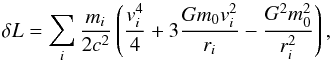 (A.2)where ri is the Heliocentric position of planet i. The general relativistic correction to the planetary Hamiltonian is thus given by δℋ = −δL (Landau & Lifshitz 1969a). To obtain the secular correction one has to average δℋ over the Keplerian orbits of the non-interacting planets. Neglecting corrections of the order mi/m0, along a Keplerian orbit one has
 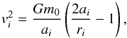 (A.3)where ai is the semimajor axis of planet i. Moreover, averaging over an orbital period one obtains
  and
and 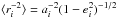 , with ei the eccentricity of planet i. Substituting Eq. (A.3)in δℋ and taking the average, one finally finds
 ![Mathematical equation: \appendix \setcounter{section}{1} \begin{equation} \label{eq:delta_Hamiltonian_average} \langle \delta \ham \rangle = \sum_i \frac{G^2 m^2_0 m_i}{c^2 a^2_i} \left[ \frac{15}{8} - \frac{3}{(1-e^2_i)^{1/2}} \right] \cdot \end{equation}](/articles/aa/full_html/2017/10/aa30916-17/aa30916-17-eq165.png) (A.4)Discarding the first term as it is constant in the secular dynamics, one obtains that the dominant secular contribution of general relativity is
(A.4)Discarding the first term as it is constant in the secular dynamics, one obtains that the dominant secular contribution of general relativity is  .
.
Appendix B: Laplace-Lagrange Hamiltonian
The matrix A appearing in the quadratic Hamiltonian (6)can be expressed as ![Mathematical equation: \appendix \setcounter{section}{2} \begin{equation} \label{eq:A} \tens{A}_{kl} = \left\{\begin{array}{@{}l@{\quad}l} - \frac{G m_k m_l a_k a_l}{\pi \sqrt{\Lambda_k \Lambda_l} |a_k - a_l|^3} I_{2kl} & \mbox{if }k \neq l \\[\jot] \sum_{\substack{j=1 \\ j \neq k}}^{N} \frac{G m_k m_j a_k a_j}{\pi \Lambda_k |a_k - a_j|^3} I_{1kj} + \frac{3 G^2 m_0^2 m_k}{c^2 a_k^2} & \mbox{if } k = l, \end{array}\right. \end{equation}](/articles/aa/full_html/2017/10/aa30916-17/aa30916-17-eq167.png) (B.1)where I have defined
(B.1)where I have defined ![Mathematical equation: \appendix \setcounter{section}{2} \begin{eqnarray*} I_{nkl} = \int_{0}^{\frac{\pi}{2}} {\rm d}\theta \frac{\cos(2n \theta)}{\left[ 1 + 4 a_k a_l \sin^2 \theta/(a_k - a_l)^2 \right]^{\frac{3}{2}}}\cdot \end{eqnarray*}](/articles/aa/full_html/2017/10/aa30916-17/aa30916-17-eq168.png) Similarly, the matrix B is given by
Similarly, the matrix B is given by ![Mathematical equation: \appendix \setcounter{section}{2} \begin{equation} \label{eq:B} \tens{B}_{kl} = \left\{\begin{array}{@{}l@{\quad}l} \frac{G m_k m_l a_k a_l}{\pi \sqrt{\Lambda_k \Lambda_l} |a_k - a_l|^3} I_{1kl} & \mbox{if }k \neq l \\[\jot] - \sum_{\substack{j=1 \\ j \neq k}}^{N} \frac{G m_k m_j a_k a_j}{\pi \Lambda_k |a_k - a_j|^3} I_{1kj} & \mbox{if } k = l. \end{array}\right. \end{equation}](/articles/aa/full_html/2017/10/aa30916-17/aa30916-17-eq169.png) (B.2)From formula (B.2)it is easy to check that matrix B verifies the following relation:
(B.2)From formula (B.2)it is easy to check that matrix B verifies the following relation:  (B.3)This implies that one of the sk eigenvalues is zero and
  is, up to a sign, the corresponding normalized eigenvector.
Appendix C: Ansatz of equiprobability: analytical description
An analytical characterization of the PDFs of eccentricity and inclination predicted by Eq. (18)can be obtained by writing the conservation of the total AMD of the inner planets, as motivated in Sect. 5, through the modified Delaunay variables (2). Compared to that of Sect. 5, such an approach does not include the statistics of giant planet orbits. The microcanonical density of states ω is then written![Mathematical equation: \appendix \setcounter{section}{3} \begin{equation} \label{eq:microcanonical_density} \frac{\omega(C_0)}{(2\pi)^{2N}} = \left[\prod_{k=1}^{N} \int_0^{\Lambda_k} \! \! \! {\rm d}P_k\! \! \int_0^{2(\Lambda_k-P_k)} \! \! \! {\rm d}Q_k \right] \delta \left( C_0 - \sum_{k=1}^N P_k + Q_k \right) , \end{equation}](/articles/aa/full_html/2017/10/aa30916-17/aa30916-17-eq173.png) (C.1)where N = 4 in the present analysis, C0 is the initial total AMD of the inner planets, and the factor (2π)2N comes from the integration over the angle variables pk and qk. Since C0< Λk for all k (Laskar 1997, Table 1), one can restrict the above integration to the hypercube [ 0,C0] 2N. To calculate the density of states one can therefore write ω(C0) = dΣ(C0)/dC0, with
(C.1)where N = 4 in the present analysis, C0 is the initial total AMD of the inner planets, and the factor (2π)2N comes from the integration over the angle variables pk and qk. Since C0< Λk for all k (Laskar 1997, Table 1), one can restrict the above integration to the hypercube [ 0,C0] 2N. To calculate the density of states one can therefore write ω(C0) = dΣ(C0)/dC0, with ![Mathematical equation: \appendix \setcounter{section}{3} \begin{equation} \label{eq:Sigma} \frac{\Sigma(C_0)}{(2\pi)^{(2N)}} = \left[\prod_{k=1}^{N} \int_0^{C_0} \! \! \! {\rm d}P_k\! \! \int_0^{C_0} \! \! \! {\rm d}Q_k \right] \, \, H \left( C_0 - \sum_{k=1}^N P_k + Q_k \right) , \end{equation}](/articles/aa/full_html/2017/10/aa30916-17/aa30916-17-eq182.png) (C.2)where H is the Heaviside step function. Performing the integrations by iteration, one obtains Σ(C0) = (2π)2NC02N/ (2N) ! and then
(C.2)where H is the Heaviside step function. Performing the integrations by iteration, one obtains Σ(C0) = (2π)2NC02N/ (2N) ! and then  (C.3)The joint microcanonical PDF of Pk and Qk (i.e. marginalized over the remaining modified Delaunay variables) is then given by
 ![Mathematical equation: \appendix \setcounter{section}{3} \begin{equation} \label{eq:rho_P_Q} \rho(P_k, Q_k) = \frac{(2\pi)^{2N}}{\omega(C_0)} \frac{{\rm d}}{{\rm d}C_0} \left[ \frac{(C_0 - P_k - Q_k)^{2N-2}}{(2N-2)!} \right] \end{equation}](/articles/aa/full_html/2017/10/aa30916-17/aa30916-17-eq188.png) (C.4)for Pk + Qk ≤ C0, otherwise it is zero. Thus one obtains
(C.4)for Pk + Qk ≤ C0, otherwise it is zero. Thus one obtains  (C.5)for Pk + Qk ≤ C0. Switching to the variables ek and ik, one finds
 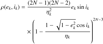 (C.6)for
 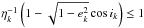 , with ηk = C0/ Λk. The PDF of ek is then given by
 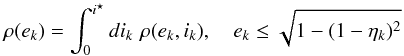 (C.7)where
 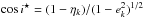 . Performing the integral, one obtains
 ![Mathematical equation: \appendix \setcounter{section}{3} \begin{equation} \label{eq:rho_ecc_2} \rho(e_k) = \frac{2N-1}{\eta_k} \frac{e_k}{\sqrt{1-e_k^2}} \left[ 1 - \eta_k^{-1} \left(1 - \sqrt{1-e_k^2} \right) \right]^{2N-2} \end{equation}](/articles/aa/full_html/2017/10/aa30916-17/aa30916-17-eq196.png) (C.8)for
(C.8)for 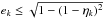 . Similarly, to obtain the PDF of ik one has to calculate
 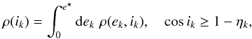 (C.9)where e⋆ = [ 1−(1−ηk)2/ cos2ik] 1/2. Performing the integration, one finds
 ![Mathematical equation: \appendix \setcounter{section}{3} \begin{eqnarray} \label{eq:rho_inc_2} \begin{split} \rho(i_k) &= \tan i_k \, \left[ 1 - \eta_k^{-1}(1-\cos i_k) \right]^{2N-2} \, \\ &\quad\times \left[ \frac{2N-1}{\eta_k}- \frac{1 - \eta_k^{-1}(1-\cos i_k)}{\cos i_k} \right] \end{split} \end{eqnarray}](/articles/aa/full_html/2017/10/aa30916-17/aa30916-17-eq200.png) (C.10)for cosik ≥ 1−ηk. As in the present study one has ηk ≪ 1 (Laskar 1997, Table 1), one can simplify these PDFs obtaining
(C.10)for cosik ≥ 1−ηk. As in the present study one has ηk ≪ 1 (Laskar 1997, Table 1), one can simplify these PDFs obtaining 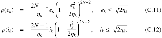 In this limit one has that
 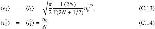 where Γ is the Gamma function, and the average AMD of planet k is thus given by
  (C.15)Therefore one obtains the equipartition of AMD between planets and between the eccentricity and inclination degrees of freedom. Even though they do not coincide, the PDFs (C.11)and (C.12)present the same overall structure as those predicted by the ansatz (18). In particular, as Eqs. (C.13)and (C.14)show, the mean and standard deviation of eccentricity and inclination are proportional to
  .
.
One can also include in the above analytical treatment the conservation of the angular momentum components Lx and Ly at quadratic order in eccentricities and inclinations (see Eq. (14)). While the shape of the eccentricity PDF is unaffected, that of the inclination PDF turns out to be somewhat influenced by the parameter  .
.
Appendix D: Ansatz of equiprobability: sampling
Conservation of AMD and energy in Eqs. (18)and (19)is equivalent to the two following conditions:  with
with  and
and  , the bar indicating the initial value of the corresponding variable (see Sect. 4 and footnote 5). These equations can be rewritten as
 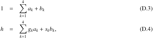 where
where  ,
,  and h = −H0/C0. Moreover, I recall that ak,bk ≥ 0, gk> 0 and sk< 0. The PDF (18)can be therefore evaluated by an uniform sampling of ak and bk verifying Eq. (D.3). To evaluate the PDF (19)ak and bk have to verify both Eqs. (D.3)and (D.4).
Uniform sampling of N positive real numbers that add up to unity, as in Eq. (D.3), can be performed via a direct sampling algorithm. One starts by sampling N−1 random numbers uniformly from the interval [0,1]. After sorting them, one obtains the set { u1,...,uN−1 }, with ui−1 ≤ ui for i ∈ { 2,...,N−1 }. Then, the numbers { u1,u2−u1,...,uN−1−uN−2,1−uN−1 } follow the target distribution.
To uniformly sampling positive real numbers ak and bk from Eqs. (D.3)and (D.4)there is probably no direct sampling method. However, I present here an efficient algorithm with rejection. Let us assume that h ≥ 0, as in the present study. A similar algorithm can be constructed in case h is negative. One can multiply Eq. (D.3)by gmax = maxk { ak }, subtract Eq. (D.4)and finally divide by gmax−h (one can assume this to be different from zero, otherwise the sampling is trivial). One obtains  (D.5)The coefficients of ak and bk in Eq. (D.5)are positive and the term ak⋆, such that gk⋆ = gmax, does not appear in it. Therefore, the other N−1 numbers can be sampled from this equation using the direct sampling algorithm presented above. If their sum S turns out to be smaller or equal to unity, then one can take ak⋆ = 1−S to obtain a set of numbers following the target distribution. Otherwise, the numbers are rejected and Eq. (D.5)sampled again.
All Tables
Parameter mk of a Rice distribution reproducing the PDF of the eccentricity of the inner planets.
All Figures
|
Fig. 1 Eccentricity and inclination PDFs of the solar system giant planets. The PDFs of L08 are plotted in solid lines, while those predicted by the microcanonical distribution function (16)are shown in dashed lines. The inclinations are computed with respect to the J2000 ecliptic. |
| In the text | |
|
Fig. 2 Eccentricity and inclination PDFs of the solar system inner planets. The PDFs of L08 are plotted in solid lines at three different times, t = 500 Myr, 2.5 Gyr, and 5 Gyr, to illustrate chaotic diffusion (the PDF broadens and its peak decreases as time increases; the inclination PDFs are not the original PDFs, but the Rice distributions fitted by Laskar, see Sect. 3 for explanations). The PDFs predicted by the microcanonical ensemble of the Laplace-Lagrange theory, Eq. (16), are shown in dashed line. The inclinations are computed with respect to the J2000 ecliptic. |
| In the text | |
|
Fig. 3 Eccentricity and inclination PDFs of the solar system inner planets. The same as Fig. 2, except that the dashed lines represent here the predictions of the ansatz (18). |
| In the text | |
|
Fig. 4 Eccentricity PDF of the Earth. The same as Fig. 3 with the addition of the prediction of Eq. (19)in dash-dotted line. |
| In the text | |
|
Fig. 5 Inclination PDF of the Earth. The same as Fig. 3 with the addition of the prediction of Eq. (19)in dash-dotted line. |
| In the text | |
|
Fig. 6 Eccentricity PDF of Mercury. The same as Fig. 3 with the addition of the predictions of Eq. (19)in dash-dotted line and Eq. (20)in dotted line. |
| In the text | |
Current usage metrics show cumulative count of Article Views (full-text article views including HTML views, PDF and ePub downloads, according to the available data) and Abstracts Views on Vision4Press platform.
Data correspond to usage on the plateform after 2015. The current usage metrics is available 48-96 hours after online publication and is updated daily on week days.
Initial download of the metrics may take a while.