| Issue |
A&A
Volume 605, September 2017
|
|
|---|---|---|
| Article Number | A38 | |
| Number of page(s) | 9 | |
| Section | Galactic structure, stellar clusters and populations | |
| DOI | https://doi.org/10.1051/0004-6361/201730545 | |
| Published online | 05 September 2017 | |
Galactic habitable zone around M and FGK stars with chemical evolution models that include dust
1 Dipartimento di Fisica, Sezione di Astronomia, Università di Trieste, via G.B. Tiepolo 11, 34131 Trieste, Italy
e-mail: This email address is being protected from spambots. You need JavaScript enabled to view it.
2 I.N.A.F. Osservatorio Astronomico di Trieste, via G.B. Tiepolo 11, 34131 Trieste, Italy
Received: 2 February 2017
Accepted: 6 May 2017
Abstract
Context. The Galactic habitable zone is defined as the region with a metallicity that is high enough to form planetary systems in which Earth-like planets could be born and might be capable of sustaining life. Life in this zone needs to survive the destructive effects of nearby supernova explosion events.
Aims. Galactic chemical evolution models can be useful tools for studying the galactic habitable zones in different systems. Our aim here is to find the Galactic habitable zone using chemical evolution models for the Milky Way disk, adopting the most recent prescriptions for the evolution of dust and for the probability of finding planetary systems around M and FGK stars. Moreover, for the first time, we express these probabilities in terms of the dust-to-gas ratio of the interstellar medium in the solar neighborhood as computed by detailed chemical evolution models.
Methods. At a fixed Galactic time and Galactocentric distance, we determined the number of M and FGK stars that host earths (but no gas giant planets) that survived supernova explosions, using the formalism of our Paper I.
Results. The probabilities of finding terrestrial planets but not gas giant planets around M stars deviate substantially from the probabilities around FGK stars for supersolar values of [Fe/H]. For both FGK and M stars, the maximum number of stars hosting habitable planets is at 8 kpc from the Galactic Center when destructive effects by supernova explosions are taken into account. Currently, M stars with habitable planets are ≃10 times more frequent than FGK stars. Moreover, we provide a sixth-order polynomial fit (and a linear fit, but that is more approximated) for the relation found with chemical evolution models in the solar neighborhood between the [Fe/H] abundances and the dust-to-gas ratio.
Conclusions. The most likely Galactic zone in which to find terrestrial habitable planets around M and FGK stars is the annular 2 kpc wide region that is centered at 8 kpc from the Galactic center (the solar neighborhood). We also provide the probabilities of finding Earth-like planets as the function of the interstellar medium dust-to-gas ratio using detailed chemical evolution model results.
Key words: Galaxy: abundances / Galaxy: evolution / planets and satellites: general / ISM: general
© ESO, 2017
1. Introduction
The Galactic habitable zone (GHZ) has been defined as the region that has sufficiently high abundances of heavy elements to form planetary systems in which terrestrial planets could be found and might be capable of sustaining life. Therefore, the chemical evolution of the Galaxy plays a key role in properly modeling the GHZ evolution in space and time. The minimum metallicity needed for planetary formation that would include the formation of a planet with Earth-like characteristics (first discussed by Gonzalez et al. 2001) has been fixed at 0.1 Z⊙ by the theoretical work of Johnson & Li (2012).
In the past years, several purely chemical evolution models (Lineweaver 2001; Lineweaver et al. 2004; Prantzos 2008; Carigi et al. 2013; Spitoni et al. 2014) have studied the habitable zones of our Galaxy as functions of the Galactic time and Galactocentric distances. In particular, Spitoni et al. (2014, hereafter Paper I) included radial gas flows in their model and confirmed the previous results of Lineweaver et al. (2004). Spitoni and colleagues found that the maximum number of stars that can host habitable terrestrial planets are located in the solar neighborhood, that is, in the region centered at 8 kpc, and this region is 2 kpc wide.
Recently, the GHZ has also been studied in the cosmological context (ΛCDM) by Forgan et al. (2017), Gobat & Hong (2016), Zackrisson et al. (2016), and Vukotić et al. (2016). These studies showed which types of halos can give rise to galactic structures in which habitable planets can be formed.
In most of the models mentioned above (both for purely chemical evolution and cosmological models), the probability of forming planetary systems in which terrestrial planets are found without any gas giant planets or hot Jupiters was considered because in principle, the last two planet types could destroy earths during their evolution.
The terms giant planets, gas giants, or simply Jupiters refer to large planets, typically >10 M⊕, that are not composed primarily of rock or other solid matter. When orbiting close to the host star, they are referred to as hot Jupiters or very hot Jupiters. The “core accretion model” of giant planet formation is the most widely accepted model in the literature, and the next stochastic migration due to turbulent fluctuations in the disk could destroy the terrestrial planets. Rice & Armitage (2003) showed that the formation of Jupiter can be accelerated by almost an order of magnitude if the growing core executes a random walk with an amplitude of ≈0.5 AU. Today, about three thousand planets have been discovered, and the statistics is to good enough to confirm that most planetary systems host planets that are not present in our solar system, such as hot Jupiters or super-Earths.
In this paper we retain the assumption that gas giant planets could destroy terrestrial planets during their evolution (we are aware that the real effects are still uncertain). On this basis, we study the GHZ using the most updated probabilities related to the formation of gas giant planets as functions of [Fe/H] abundance values as well as the stellar mass for FGK and M stars. Recently, a planetary system around the M star Trappist-1 has been discovered (Gillon et al. 2016, 2017). This system is composed of seven terrestrial planets characterized by an equilibrium temperature low enough to allow liquid water. This detection makes the habitability around M stars even more interesting.
In this paper we also compute the probabilities related to the formation of gas giant planets as functions of [Fe/H] abundance values and the stellar mass for FGK and M stars. We describe a detailed chemical evolution model for the Milky Way that includes dust evolution.
We know very little about the formation of planetary systems. In particular, the transition from a protoplanetary disk to a planetary system is poorly understood. In this transition, dust and gas rapidly evolve in very different ways as a result of many processes (Armitage 2013) such as dust growth, gas photoevaporization (Alexander et al. 2014), and gas accretion onto the star (Gammie 1996). Dust plays a fundamental role in the formation of the first planetesimals because it represents the solid compounds of the matter that can form rocky planetesimals and therefore planets.
The first fundamental step to understand and explain the origin of the observed diversity of exoplanetary systems is to measure the stellar disk properties, especially the disk mass. Dust grains of μm size are directly observed in protoplanetary disks and then, dust coagulation increases their size up to mm (Dullemond & Dominik 2005). On the other hand, observations of the gas are almost forbidden because it is relatively cool and in molecular form.
In most cases, the mass of the gas is set starting from the gas mass of the dust and by assuming a value for the dust-to-gas ratio. Unfortunately, this practice has several uncertainties (Williams & Best 2014). Models of planetary formation commonly use an average value of 10-2 for the initial condition of the dust-to-gas ratio in the protoplanetary disk (Bohlin et al. 1978).
Furthermore, the formation rate of gas giant planets seems to be related to the metallicity of the hosting stars (Fisher & Valenti 2005; Johnson et al. 2010; Mortier et al. 2012; Gaidos & Mann 2014). Moreover, even though Buhhave et al. (2012) showed that planets with radii smaller than 4 R⊕ do not present any metallicity correlation, the theoretical work of Johnson & Li (2012) predicted that first Earth-like planets likely formed from circumstellar disks with metallicities Z ≥ 0.1Z⊙.
We here provide the time evolution of the dust and discuss the connection between the metallicity of the interstellar medium (ISM) and the dust-to-gas D/G (especially for the solar neighborhood). In this way, we can link the metallicity of stars, which is observationally related to the probability of the presence of hosted planets, with the initial dust-to-gas ratio of the protoplanetary disks (the dust-to-gas ratio of the ISM at the instant of the protoplanetary disk formation).
The paper is organized as follows: in Sect. 2 we present the probabilities of terrestrial planets around M and FGK stars. In Sect. 3 we describe the Milky Way chemical evolution model including dust, and we present the main results in Sect. 4. Finally, our conclusions are summarized in Sect. 5.
2. Probabilities of terrestrial planets around M and FGK stars
Buchhave et al. (2012) analyzed the Kepler mission and found that the frequencies of the planets with Earth-like sizes are almost independent of the metallicity of the host star up to [Fe/H] abundance values lower than 0.5 dex.
In agreement with these observations, Prantzos (2008) fixed the probability of forming Earth-like planets (PFE, where FE stands for “forming earths”) at a value of 0.4 for [ Fe / H ] ≥ − 1 dex, otherwise PFE = 0 for lower values of [Fe/H]. This assumption was also adopted by Carigi et al. (2013) and in Paper I. The value of PFE = 0.4 was chosen to reproduce the metallicity-integrated probability of Lineweaver et al. (2001).
In Paper I we considered the case in which gaseous giant planets with the same host star can destroy terrestrial planets (i.e., during their migration path). Armitage (2003) pointed out the potentially hazardous effects of the gas giant planet migration on the formation of Earth-like planets and suggested that these planets preferentially exist in systems where massive giants did not migrate significantly. Matsumura et al. (2013) studied the orbital evolution of terrestrial planets when gas giant planets become dynamically unstable. The authors showed that Earth-like planets far away from giants can also be removed.
On the other hand, various numerical simulations found that the formation of earths is not necessarily prevented by the gas giant planet migration, when eccentricity excitation timescales for (proto-)terrestrial planets are longer than the migration timescales of giant planets (e.g., Mandell & Sigurdsson 2003; Lufkin et al. 2006; Raymond et al. 2006).
The adopted probability of the formation of a gaseous giant planet as a function of the iron abundance in the host star is taken by Fischer & Valenti (2005) as ![Mathematical equation: \begin{equation} P_{\rm GGP}\left(\mbox{[Fe/H}]\right)= 0.03 \times 10^{2.0 \mbox{[Fe/H]}}. \label{valenti} \end{equation}](/articles/aa/full_html/2017/09/aa30545-17/aa30545-17-eq16.png) (1)A possible theoretical explanation is that the high metallicity observed in some stars hosting giant planets represents the original composition in which protostellar and protoplanetary molecular clouds were formed. In this scenario, the higher the metallicity of the primordial cloud, the higher the proportion of dust to gas in the protoplanetary disk. This facilitates the condensation and accelerates the protoplanetary accretion before the disk gas is lost (Pollack et al. 1996). Giant planets are subsequently formed by runaway accretion of gas onto such rocky cores with M ≈ 10 M⊕ instead of by gravitational instabilities in a gaseous disk, which predicts a formation that is much less sensitive to metallicity (Boss 2002).
(1)A possible theoretical explanation is that the high metallicity observed in some stars hosting giant planets represents the original composition in which protostellar and protoplanetary molecular clouds were formed. In this scenario, the higher the metallicity of the primordial cloud, the higher the proportion of dust to gas in the protoplanetary disk. This facilitates the condensation and accelerates the protoplanetary accretion before the disk gas is lost (Pollack et al. 1996). Giant planets are subsequently formed by runaway accretion of gas onto such rocky cores with M ≈ 10 M⊕ instead of by gravitational instabilities in a gaseous disk, which predicts a formation that is much less sensitive to metallicity (Boss 2002).
The novelty of our work is that we consider the following new probabilities for gas giant planets formation reported by Gaidos & Mann (2014) that were used by Zackrisson et al. (2016) around FGK and M stars. These probabilities are also functions of the masses of the hosting stars, ![Mathematical equation: \begin{equation} P_{\rm GGP/FGK}\left(\mbox{[Fe/H}], M_{\star}\right)= 0.07 \times 10^{1.8 \mbox{[Fe/H]}} \left( \frac{M_{\star}}{M_{\odot}}\right) \label{eqgiantF} \end{equation}](/articles/aa/full_html/2017/09/aa30545-17/aa30545-17-eq18.png) (2)for the FGK stars, and
(2)for the FGK stars, and ![Mathematical equation: \begin{equation} P_{\rm GGP/M}\left(\mbox{[Fe/H}], M_{\star}\right)= 0.07 \times 10^{1.06 \mbox{[Fe/H]}} \left( \frac{M_{\star}}{M_{\odot}}\right) \label{eqgiantM} \end{equation}](/articles/aa/full_html/2017/09/aa30545-17/aa30545-17-eq19.png) (3)for M stars, where M⋆ is the mass of the host star in units of solar masses.
(3)for M stars, where M⋆ is the mass of the host star in units of solar masses.
We assume that the range of masses spanned by M-type stars is  . For the FGK stars, the range is
  .
.
The probability of forming terrestrial planets around FGK/M stars but not gaseous giant planets is given by  (4)Here, we adopt the conservative assumption of Prantzos (2008) and Paper I that the PFE probability is constant at the value of 0.4 for all stellar types, including M and FGK stars. On the other hand, Zackrisson et al. (2016) presented results where PFE = 0.4 around FGK stars, and PFE = 1 around M stars.
The possibility of finding habitable planets around M-dwarf stars has long been debated because there are differences between the unique stellar and planetary environments around these low-mass stars compared to hotter, more luminous Sun-like stars (Shields et al. 2016). The presence of multiple rocky planets (Howard et al. 2012), with roughly a third of these rocky M-dwarf planets orbiting within the habitable zone, supports the hypothesis of the presence of liquid water on their surfaces. On the other hand, flare activity, synchronous rotation, and the likelihood of photosynthesis could have a severe effect on the habitability of planets hosted by M-dwarf stars (Tarter et al. 2007).
We define PGHZ(FGK / M,R,t) as the fraction of all FGK/M stars that host Earths (but no gas giant planets) that survived supernova (SN) explosions as a function of the Galactic radius and time:
 (5)
(5)
This quantity must be interpreted as the relative probability to have complex life around one star at a given position, as suggested by Prantzos (2008).
In Eq. (5), SFR(R,t′) is the star formation rate (SFR) at the time t′ and Galactocentric distance R, and PSN(R,t′) is the probability of surviving an SN explosion.
We know that hard radiation caused by close-by SN explosions could lead to the depletion of the ozone layer in a terrestrial atmosphere. At this point, the ultraviolet radiation from the host star can penetrate the atmosphere, altering and damaging the DNA and eventually causing the total sterilization of the planet (Gehrels et al. 2003).
For this quantity we refer to the “case 2” model of Paper I in which the SN destruction is effective if the SN rate at any time and at any radius has been higher than twice the average SN rate in the solar neighborhood during the last 4.5 Gyr of the Milky Way life (we call it ⟨ RSNSV ⟩).
Therefore, we impose that if the SN rate is higher than 2 × ⟨ RSNSV ⟩ , then PSN(R,t) = 0, else PSN(R,t) = 1. We also show results when SN effects are not taken into account. In this case, we simply impose PSN(R,t) = 1 at any time and galactic radius. The case 2 condition is almost the same as the condition used by Carigi et al. (2013) to describe their best models, motivated by the fact that life on Earth has proven to be highly resistant, and the real effects of SN explosions on life are still extremely uncertain.
For ⟨ RSNSV ⟩ we adopt the value of 0.01356 Gyr-1 pc-2 using the results of the S2IT model of Spitoni & Matteucci (2011) and Paper I.
Finally, we define the total number of stars formed at a certain time t and Galactocentric distance R that host an Earth-like planet with life N⋆ life(FGK / M,R,t) as  (6)where N⋆ tot(FGK / M,R,t) is the total number of stars created up to a time t at the Galactocentric distance R.
3. Milky Way chemical evolution model that includes dust
To trace the chemical evolution of the Milky Way, we adopt an updated version of the two-infall model of Paper I, in which we consider the dust evolution using the new prescriptions of Gioannini et al. (2017).
3.1. Two-infall model of Paper I
The chemical evolution model of Paper I is based on the classical two-infall model of Chiappini et al. (2001). We describe here the main characteristics of the model.
We define Gi(t) = G(t)Xi(t) as the fractional mass of the element i at the time t in the ISM, where Xi(t) represents the abundance of the element i in the ISM at the time t. The temporal evolution of Gi(t) in the ISM is described by the following expression:  (7)The first term on the right side of Eq. (7) represents the rate at which the fraction of the element i is subtracted by the ISM due to the SFR process. Ri(t) is the returned mass fraction of the element i injected into the ISM from stars thanks to stellar winds and SN explosions. This term takes into account nucleosynthesis prescriptions concerning stellar yields and supernova progenitor models. The third term of Eq. (7) represents the rate of the infall of the element i. The infalling gas is not pre-enriched and has a pure primordial composition.
The two-infall approach is a sequential model in which the halo thick disk and the thin disk form by means of two independent infall episodes of primordial gas following this infall rate law:  (8)where τH is the typical timescale for the formation of the halo and thick disk, and it is fixed to the value of 0.8 Gyr, while tmax = 1 Gyr is the time for the maximum infall onto the thin disk. The coefficients a(r) and b(r) are obtained by imposing a fit to the observed current total surface mass density in the thin disk as a function of Galactocentric distance given by
  (9)where Σ0 = 531 M⊙ pc-2 is the central total surface mass density and RD = 3.5 kpc is the scale length. Moreover, the formation timescale of the thin disk τD(r) is assumed to be a function of the Galactocentric distance, leading to an inside-out scenario for the Galaxy disk build-up. In particular, we assume that
  (10)The Galactic thin disk is approximated by several independent rings, 2 kpc wide, without exchange of matter between them. A threshold gas density of 7 M⊙ pc-2 in the SF process (Kennicutt 1989, 1998; Martin & Kennicutt 2001; Schaye 2004) is also adopted for the disk. The halo has a constant surface mass density as a function of the Galactocentric distance at the present time equal to 17 M⊙ pc-2 and a threshold for the star formation in the halo phase of 4 M⊙ pc-2, as assumed for model B of Chiappini et al. (2001).
The assumed IMF is the one of Scalo (1986), which is assumed to be constant in time and space.
For the SFR we adopted the law of Schmidt (1959),  (11)where Σgas(r,t) is the surface gas density with the exponent k equal to 1.5 (see Kennicutt 1998; and Chiappini et al. 1997). The quantity ν is the efficiency of the star formation process, and it is constant and fixed to be equal to 1 Gyr-1. The chemical abundances are normalized to the solar values of Asplund et al. (2009).
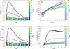 |
Fig. 1 Panel A: SFR as the function of the Galactic time. Panel B: time evolution of the [Fe/H] abundances with the two-infall chemical evolution model for the Milky Way disk (the “age-metallicity” relation). Panel C: evolution in time of the type II SN rates plus the type Ia SN rates. With the red line we show the quantity 2 × ⟨ RSNSV ⟩ , which represents the minimum SN rate value (adopted in this work and in Paper I) for destruction effects from SN explosions. Panel D: time evolution of the total dust surface mass density. The color code in the four panels indicates the different Galactocentric distances. |
3.2. Evolution of dust
Our chemical evolution model also traces the dust evolution in the ISM. Defining Gi,dust(t), we can thus write the equation for dust evolution as follows: 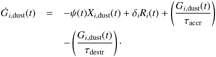 (12)The right-hand side of this equation contains all the processes that govern the so-called “dust cycle”: the first term represents the amount of dust removed from the ISM as a result of star formation, the second takes into account dust pollution by stars, while the third and fourth terms represent dust accretion and destruction in the ISM, respectively. In this work, we used the same prescriptions as in Gioannini et al. (2017). Dust production is provided by taking condensation efficiencies δi1 as provided by Piovan et al. (2011) into account.
The dust yields δiRi(t) are not only metallicity dependent, but also depend on the mass of the progenitor star. In this work we consider as dust producers type II SNe (M⋆> 8 M⊙) and low- to intermediate-mass stars (1.0 M⊙<M⋆< 8.0 M⊙). For dust accretion and destruction, we calculated the metallicity-dependent timescales for these processes (τaccr and τdestr) as described in Asano et al. (2013). For a more detailed explanation of dust prescriptions or dust chemical evolution model, we refer to Gioannini et al. (2017).
4. Results
In this section we first present the main results of our Milky Way chemical evolution model when dust is included. Moreover, we show the PE / FGK,M probabilities of finding Earth-like planets, but no gas giants around FGK and M stars of Gaidos & Mann (2014), computed with detailed chemical evolution models for the Galactic disk at different Galactocentric distances. We express these probabilities in terms of the dust-to-gas ratio  obtained by our ISM chemical evolution models. Finally, we present the maps of habitability of our Galaxy as functions of Galactic time and Galactocentric distances in terms of the total number of FGK and M stars that could host habitable Earth-like planets and not gas giant planets.
4.1. Milky Way disk with dust
In Fig. 1 we show the time evolution of the SFR (panel A), the [Fe/H] abundances (panel B), the SN rates (panel C), and finally of the total dust (panel D) as functions of the Galactocentric distance. In panel A we see the effect of the inside-out formation on the SFR in the thin-disk phase. During the halo and thick-disk phase (up to 1 Gyr since the beginning of the star formation), all the Galactocentric distances show the same star formation history (for all radii we assume the same surface gas density and same formation timescales in the halo and thick-disk phase, for details see Sect. 3).
In the inner regions the SFR in the thin-disk phase is higher because the gas density is higher and the gas accretion timescale is longer than in the outer regions. In the outer regions the effect of the threshold on the gas density is more pronounced: the SFR reaches zero when the gas density is below the threshold. We also note that the same SFR history is obtained at all Galactocentric distances in the halo and thick-disk phase.
In panel B we show the age-metallicity relation in terms of [Fe/H] ratio vs. Galactic time. The effects of the inside-out formation are clear in this case as well: the inner regions exhibit a faster and more efficient chemical enrichment, with higher values of [Fe/H]. At early times, in correspondence to the beginning of the second infall of gas (thin-disk phase), the [Fe/H] abundance values decrease. This decrease is more evident in the inner regions of the Galactic disk. The reason is that the second infall of primordial gas related to the thin-disk phase is more massive in the inner regions and it occurs on shorter timescales, therefore the chemical abundances are more diluted at the beginning of the thin-disk phase in the inner Galactic regions than in the external regions.
In panel C of Fig. 1 we present the total SN rates as functions of the Galactic time and Galactocentric distances. With the red line we show the limit we adopted here and in Paper I to take the destruction effects of SN explosions on the Galactic habitable zone modeling into account (2 × ⟨ RSNSV ⟩). Above this SN rate limit, we assume that there is zero probability of life on a terrestrial planet.
Finally, in panel D of Fig. 1 we show the time evolution of the total surface mass density of dust at different Galactocentric radii. Dust production by stars is the main source of dust in the early phases of the Milky Way evolution. For this reason, in the inner regions, the dust amount is higher because type II SNe during the initial burst of star formation produce more dust, as is visible in panel A. On the other hand, dust accretion becomes important at later epochs, and the dust mass tends to increase at all Galactocentric distances. The observed oscillation of the model occurs when the rates of dust accretion and dust destruction are similar. In this case, there is a gain of the total mass surface density of dust caused by the dust growth, rapidly followed by a decrease that is due to the dust destruction rate, which exceeds dust accretion. This turnover between these processes occurs especially in the quiescent phases of the Galactic evolution.
4.2. Computed probabilities PGGP/FGK,M with the two-infall chemical evolution model
To compute the probabilities PGGP / FGK,M presented in Eqs. (2) and (3) with our chemical evolution model, we considered the weighted values on the IMF using the following expressions:
![Mathematical equation: \begin{eqnarray} &&\langle P_{\rm GGP/FGK}(R,t)\rangle_{\rm IMF}= \nonumber\\ &&\qquad \qquad 0.07 \times 10^{1.8 \mbox{[Fe/H]}(R,t)_{\rm model}} \left( \left\langle \frac{M_{\star,\rm FGK}}{M_{\odot}}\right\rangle_{\rm IMF}\right) \end{eqnarray}](/articles/aa/full_html/2017/09/aa30545-17/aa30545-17-eq79.png) (13)for the FGK stars, and
(13)for the FGK stars, and ![Mathematical equation: \begin{eqnarray} &&\langle P_{\rm GGP/M}(R,t)\rangle_{\rm IMF}= \nonumber\\ &&\qquad 0.07 \times 10^{1.06 \mbox{[Fe/H]}(R,t)_{\rm model}} \left( \left\langle\frac{M_{\star, M}}{M_{\odot}}\right\rangle_{\rm IMF}\right) \end{eqnarray}](/articles/aa/full_html/2017/09/aa30545-17/aa30545-17-eq80.png) (14)for M stars.
(14)for M stars.
The [Fe/H](R,t)model quantity is the computed iron abundance with our chemical evolution model adopting the Scalo (1986) IMF at the Galactic time t and Galactocentric distance R.
Therefore, to compute ⟨ PGGP / M ⟩ IMF and ⟨ PGGP / FGK ⟩ IMF quantities, we have only to know the weighted stellar mass on the IMF in the mass range of M and FGK stars, respectively. The weighted stellar masses on the Scalo (1986) IMF are 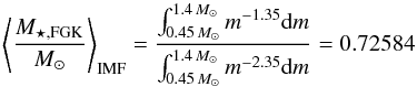 (15)and
 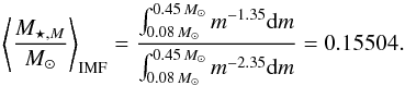 (16)In Fig. 2 we show the evolution of ⟨ PGGP / FGK ⟩ IMF and ⟨ PGGP / M ⟩ IMF probabilities as a function of the [Fe/H] abundance ratio computed at different Galactocentric distances using our chemical evolution models. Because of the inside-out formation, the inner regions exhibit a faster and more efficient chemical enrichment. The model computed at 4 kpc reaches at the present time [Fe/H] value of 0.55 dex; instead, at 20 kpc, the maximum [Fe/H] is equal to –0.1 dex. We see that the two probabilities are substantially different for super-solar values in the inner regions. For instance, at the present time, that is, at the maximum values of the [Fe/H] abundance in panel C of Fig. 1, at 4 kpc, the probabilities ⟨ PGGP / FGK ⟩ IMF and ⟨ PGGP / M ⟩ IMF show values of 0.43 and 0.04, respectively.
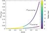 |
Fig. 2 Probabilities ⟨ PGGP / FGK ⟩ IMF and ⟨ PGGP / M ⟩ IMF of finding gas giant planets around FGK and M stars, respectively, as functions of the abundance ratio [Fe/H] using our chemical evolution model for the Milky Way disk and adopting the prescriptions given by Gaidos & Mann (2014). The color code indicates the Galactocentric distance. |
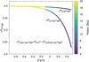 |
Fig. 3 Probabilities ⟨ PE / FGK ⟩ IMF and ⟨ PE / M ⟩ IMF of finding terrestrial planets but not gas giant planets around FGK and M stars, respectively, as functions of the abundance ratio [Fe/H] using our chemical evolution model for the Milky Way disk and adopting the prescriptions given by Gaidos & Mann (2014) and Paper I. The color code indicates the Galactocentric distance. |
4.3. Dust-to-gas ratio D/G
In this subsection we provide a useful theoretical tool to set the proper initial conditions for the formation of protoplanetary disks. As underlined in Sect. 1, while dust grains of μm are directly observed in protoplanetary disks, the amount of gas mass is set starting from the dust mass and by assuming a value for the dust-to-gas ratio. Unfortunately, this practice has several uncertainties (Williams & Best 2014). In this subsection, we connect the evolution of the dust-to-gas ratios at different Galactocentric distances with the chemical enrichment expressed in terms of [Fe/H]. Because of the well-known age-metallicity relation reported in panel C of Fig. 1, the dust-to-gas ratio (D/G) vs. [Fe/H] abundance ratio relation can be seen as a time evolution for the dust-to-gas ratio (D/G)(t).
In the upper panel of Fig. 4 we present the evolution of the dust-to-gas ratio D/G as a function of [Fe/H] at different Galactocentric distances. As expected, higher metallicities are reached in the inner radii, where the star formation is higher. The dust-to-gas ratio D/G increases in time for two reasons: the first is that dust production in star-forming regions is high, especially from type II SNe, while the second reason is related to dust accretion. Dust accretion is a very important process occurring in the ISM, and it becomes the most important process when the critical metallicity is reached2.
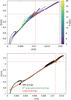 |
Fig. 4 Upper panel: evolution of the abundance ratio [Fe/H] as a function of the dust-to-gas ratio D/G predicted by our chemical evolution model of the Milky Way disk. As in Fig. 1, the color code indicates different Galactocentric distances. Lower panel: with the black solid line we report the [Fe/H] ratio vs. |

As dust grains are formed by metals, dust accretion becomes more efficient as the metallicity in the ISM increases. For this reason, we found higher values of dust-to-gas ratio at high values of [Fe/H]. The relation between the [Fe/H] and the dust-to-gas ratio is important because it can provide the probability of planet formation depending on the amount of dust in the ISM, and on the other hand, it provides an estimate of the dust-to-gas ratio in the ISM during the formation of a protoplanetary disk.
The solar dust-to-gas ratio  value predicted by our model (model value computed in the solar neighborhood at 9.5 Gyr) is 0.01066.
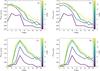 |
Fig. 5 Upper panels: probability ⟨ PGHZ ⟩ IMF of finding terrestrial habitable planets, but not gas giant around FGK stars (panel A) and M stars (panel B) as a function of the Galactocentric radius. In this case, we do not consider the destructive effects from nearby SN explosions. The color code indicates different Galactic times. Lower panels: probability PGHZ of finding terrestrial habitable planets, but not gas giant around FGK stars (panel C) and M stars (panel D) as a function of the Galactocentric radius, taking the destructive effects from nearby SN explosions into account. The color code indicates different Galactic times. |
In the lower panel of Fig. 4 we show the D/G as a function of the [Fe/H] values only for the shell centered at 8 kpc and 2 kpc wide (the solar neighborhood). In the same plot, we present the sixth-degree polynomial fit that exactly follows the [Fe/H] vs. (D/G) in the range of [Fe/H] between –1 dex and 0.5 dex. The expression of this fit is ![Mathematical equation: \begin{equation} \mbox{[Fe/H]}=\sum_{n=0}^{6} \alpha_n \left(\frac{D}{G}\right)^n \cdot \end{equation}](/articles/aa/full_html/2017/09/aa30545-17/aa30545-17-eq94.png) (17)All the coefficients αn and n are reported in the footnote 3.
(17)All the coefficients αn and n are reported in the footnote 3.
We found that for [Fe/H] values higher than –0.6 dex a linear fit is able to reproduce the computed [Fe/H] vs.  relation in the solar vicinity well.
The equation of the linear fit reported in the lower panel of Fig. 4 is ![Mathematical equation: \begin{equation} \mbox{[Fe/H]}=96.49 \left( \frac{D}{G} \right) -0.92. \end{equation}](/articles/aa/full_html/2017/09/aa30545-17/aa30545-17-eq98.png) (18)This relation is important to connect the dust-to-gas ratio with the [Fe/H] abundance. When we combine it with Eq. (4), we obtain the probability of having terrestrial planets, but no gas giants, depending on the amount of dust in the ISM.
(18)This relation is important to connect the dust-to-gas ratio with the [Fe/H] abundance. When we combine it with Eq. (4), we obtain the probability of having terrestrial planets, but no gas giants, depending on the amount of dust in the ISM.
4.4. PGHZ values around FGK and M stars
In the upper panels of Fig. 5 (A and B) we show the evolution in time of the PGHZ values for FGK and M stars as functions of the Galactocentric distance when SN destruction effects are not taken into account.
We note that the ⟨ PGHZ / M ⟩ IMF and ⟨ PGHZ / FGK ⟩ IMF probabilities are identical at large Galactocentric distances. As shown in Fig. 3, the reason is that the ⟨ PE / FGK ⟩ IMF and ⟨ PE / M ⟩ IMF probabilities are similar for sub-solar values of [Fe/H]. The chemical evolution in the outer parts of the Galaxy, is slow and has longer timescales because of the inside-out formation. The maximum values of [Fe/H] are lower than in the inner region and are sub-solar (see the age-metallicity relation reported in panel B of Fig. 1).
Moreover, in the inner regions, the ⟨ PGHZ,M ⟩ IMF and ⟨ PGHZ,FGK ⟩ IMF probabilities become different only for Galactic times longer than 8 Gyr. As expected, the higher probabilities are related to the M stars. Even when the ⟨ PE / FGK ⟩ IMF and ⟨ PE / M ⟩ IMF probabilities are substantially different for [Fe/H] > 0.2 (see Fig. 3), the two associated PGHZ probabilities are similar.
The reason is the definition of PGHZ(t): at each Galactic time, the SFR × PE quantity is integrated from 0 to t. In other words, we are weighting the PE quantity on the SFR. From panel C of Fig. 1 it is clear that the peak of the SFR in the inner regions (annular region between 3 and 7 kpc) is around 3 Gyr. From the age-metallicity relation reported in panel B of Fig. 1, we derive that at this age, the mean Galactic [Fe/H] is –0.5 dex. At this metallicity, as stated above, the PE.FGK and PE.M values are almost the same. This is the reason why the two PGHZ probabilities are similar even at late time in the inner regions.
In the lower panels of Fig. 5 (C and D) we show that the PGHZ probabilities for FGK and M stars as functions of the Galactocentric distances and time are almost identical when the SN destruction effects have been taken into account. As we found in Paper I, the Galactocentric distance with the highest probability that a star (FGK or M type) hosts a terrestrial planet, but no gas giants, is 10 kpc.
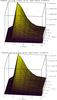 |
Fig. 6 Total number of FGK stars (upper panel) and M stars (lower panel) with habitable terrestrial planets, but no gas giants, as functions of the Galactocentric distance and the Galactic time (the N⋆ life quantity in Eq. (6)) where SN destructive effects are taken into account. The number of stars is computed within concentric rings that are 2 kpc wide. |
4.5. GHZ maps for FGK and M stars
In order to recover the total number of stars at the Galactic time t and Galactocentric distance R that host habitable planets, the total number of stars created up to time t at the Galactocentric distance R (N⋆ tot quantity in Eq. (6)) is required.
Our chemical evolution model reproduces the observed total local stellar surface mass density of 35 ± 5 M⊙ pc-2 very well (Gilmore et al. 1989; Spitoni et al. 2015). Our predicted value for the total surface mass density of stars is 35.039 M⊙ pc-2. Moreover, we find that this value for M stars alone is 24.923 M⊙ pc-2 and the value for FGK stars is 9.579 M⊙ pc-2.
In Fig. 6 we show the number of FGK stars (upper panel) and M stars (lower panel) that host habitable terrestrial planets, but no gas giant planets, as functions of the Galactic time and Galactocentric radius (quantity N⋆ life of Eq. (6)).
We note that for both FGK and M stars, the GHZ maps, in terms of the total number of stars that host planets with life, peaks at 8 kpc. On the other hand, as we showed above, the maximum fraction of stars that can host habitable terrestrial planets peaks at 10 kpc (see panels C and D of Fig. 5).
The reason why the GHZ peaks at galactocentric smaller distances than when it is expressed in terms of the fraction of stars is that in the external regions, the number of stars formed at any time is smaller than in the inner regions because the SFR is lower. This is in agreement with the results of Prantzos (2008) and Paper I.
We see that at the present time, in the solar neighborhood the number N⋆,M,life/N⋆,FGK,life = 10.60. This ratio is consistent with the IMF we adopted in our model. The ratio between the fraction of M stars over FGK stars (by number) in a newborn population adopting a Scalo IMF is 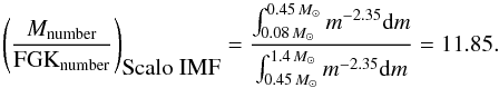 (19)Finally, the predicted local surface mass density of M stars that host habitable planets predicted by our model is 5.446 M⊙ pc-2, and the value for FGK stars is 2.40 M⊙ pc-2.
5. Conclusions
We investigated the Galactic habitable zone of the Milky Way by adopting the most updated prescriptions for the probabilities of finding terrestrial planets and gas giant planets around FGK and M stars. To do this, we adopted a chemical evolution model for the Milky Way that follows the evolution of the chemical abundances both in the gas and dust.
The main results can be summarized as follows:
-
When we adopt the Scalo (1986) IMF, the probabilities of findinggas giant planets around FGK and M stars computed with thetwo-infall chemical evolution model of Paper I begin to bedifferent for super-solar values of [Fe/H]. In particular,substantial differences are present in the annular region centeredat 4 kpc from the Galactic center.
-
We provide for the first time a sixth-order polynomial fit (and a linear fit, but this is more approximated) for the relation found in the chemical evolution model in the solar neighborhood between the [Fe/H] abundances and the dust-to-gas ratio D/G. With this relation, it is possible to express the Gaidos & Mann (2014) probabilities of finding gaseous giant planets around FGK or M stars in terms of the gas-to-dust ratio D/G.
-
We provide a useful theoretical tool to set the proper initial condition for the formation of protoplanetary disks by connecting the evolution of the dust-to-gas ratios at different Galactocentric distances with the chemical enrichment expressed in terms of [Fe/H].
-
The probabilities that an FGK or M star could host habitable planets are roughly identical. Slight differences arise only at Galactic times longer than 9 Gyr, where the probability of finding gas giant planets around FGK becomes substantially different from the probability associated with M stars.
-
As found by Paper I, adopting the same prescriptions for the destructive effect from close-by SN explosions, the larger number of FGK and M stars with habitable planets are found in the solar neighborhood.
-
At the present time, the total number of M stars with habitable terrestrial planets without gas giants are ≃10 times the number of FGK stars. This result is consistent with the Scalo (1986) IMF adopted here.
The Gaia mission with its global astrometry will be crucial for the study of exoplanets. We recall that the relation used in this work between the frequency of gas giant planets and the metallicity of the host star was obtained by means of the Doppler effect with the method of radial velocity, and it will be possible with Gaia to test whether this result is an observational bias or is related to real physical processes. It is estimated that Gaia will be able to find out up to 104 giant planets in the solar vicinity with its global astrometry, with distances spanning the range between 0.5 and 4.5 AU from the host star.
The condensation efficiency (δi) represents the fraction of an element i expelled from a star that reaches the dust phase of the ISM.
The critical metallicity is the metallicity at which the contribution of dust accretion exceeds the dust production from stars (Asano et al. 2013).
[Fe/H] =  .
.
Acknowledgments
We thank the anonymous referee for the suggestions that improved the paper. The work was supported by PRIN MIUR 2010-2011, project “The Chemical and dynamical Evolution of the Milky Way and Local Group Galaxies”, prot. 2010LY5N2T.
References
- Alexander, R., Pascucci, I., Andrews, S., Armitage, P., & Cieza, L. 2014, Protostars and Planets VI (Tucson: University of Arizona Press), 475 [Google Scholar]
- Armitage, P. J. 2003, ApJ, 582, L47 [NASA ADS] [CrossRef] [MathSciNet] [Google Scholar]
- Armitage, P. J. 2013, Astrophysics of Planet Formation (Cambridge, UK: Cambridge University Press) [Google Scholar]
- Asano, R. S., Takeuchi, T. T., Hirashita, H., & Nozawa, T. 2013, MNRAS, 432, 637 [NASA ADS] [CrossRef] [Google Scholar]
- Asplund, M., Grevesse, N., Sauval, A. J., & Scott, P. 2009, ARA&A, 47, 481 [NASA ADS] [CrossRef] [Google Scholar]
- Bohlin, R. C., Savage, B. D., & Drake, J. F. 1978, ApJ, 224, 132 [NASA ADS] [CrossRef] [Google Scholar]
- Boss, A. P. 2002, ApJ, 567, L149 [Google Scholar]
- Buchhave, L. A., Latham, D. W., Johansen, A., et al. 2012, Nature, 486, 375 [NASA ADS] [Google Scholar]
- Carigi, L., Garcia-Rojas, J., & Meneses-Goytia, S. 2013, Rev. Mex. Astron. Astrofis., 49, 253 [Google Scholar]
- Chiappini, C., Matteucci, F., & Gratton, R. 1997, ApJ, 477, 765 [NASA ADS] [CrossRef] [Google Scholar]
- Chiappini, C., Matteucci, F., & Romano, D. 2001, ApJ, 554, 1044 [NASA ADS] [CrossRef] [Google Scholar]
- Dullemond, C. P., & Dominik, C. 2005, A&A, 434, 971 [NASA ADS] [CrossRef] [EDP Sciences] [Google Scholar]
- Fischer, D. A., & Valenti, J. 2005, ApJ, 622, 1102 [NASA ADS] [CrossRef] [Google Scholar]
- Forgan, D., Dayal, P., Cockell, C., & Libeskind, N. 2017, Int. J. Astrobiol., 16, 60 [CrossRef] [Google Scholar]
- Gaidos, E., & Mann, A. W. 2014, ApJ, 791, 54 [NASA ADS] [CrossRef] [Google Scholar]
- Gammie, C. F. 1996, ApJ, 457, 355 [NASA ADS] [CrossRef] [Google Scholar]
- Gehrels, N., Laird, C. M., Jackman, C. H., et al. 2003, ApJ, 585, 1169 [NASA ADS] [CrossRef] [Google Scholar]
- Gilmore, G., Wyse, R. F. G., & Kuijken, K. 1989, ARA&A, 27, 555 [NASA ADS] [CrossRef] [Google Scholar]
- Gioannini, L., Matteucci, F., Vladilo, G., & Calura, F. 2017, MNRAS, 464, 985 [NASA ADS] [CrossRef] [Google Scholar]
- Gillon, M., Jehin, E., Lederer, S. M., et al. 2016, Nature, 533, 221 [NASA ADS] [CrossRef] [PubMed] [Google Scholar]
- Gillon, M., Triaud, A. H. M. J., Demory, B. O., et al. 2017, Nature, 542, 456 [NASA ADS] [CrossRef] [PubMed] [Google Scholar]
- Gobat, R., & Hong, S. E. 2016, A&A, 592, A96 [NASA ADS] [CrossRef] [EDP Sciences] [Google Scholar]
- Gonzalez, G., Brownlee, D., & Ward, P. 2001, Icarus, 152, 185 [NASA ADS] [CrossRef] [Google Scholar]
- Howard, A. W., Marcy, G. W., Bryson, S. T., et al. 2012, ApJS, 201, 15 [NASA ADS] [CrossRef] [Google Scholar]
- Johnson, J. A., Aller, K. M., Howard, A. W., & Crepp, J. R. 2010, PASP, 122, 905 [NASA ADS] [CrossRef] [Google Scholar]
- Johnson, J. L., & Li, H. 2012, ApJ, 751, 81 [NASA ADS] [CrossRef] [Google Scholar]
- Kennicutt, R. C., Jr 1989, ApJ, 344, 685 [NASA ADS] [CrossRef] [Google Scholar]
- Kennicutt, R. C., Jr 1998, ApJ, 498, 541 [NASA ADS] [CrossRef] [Google Scholar]
- Lineweaver, C. H. 2001, Icarus, 151, 307 [NASA ADS] [CrossRef] [Google Scholar]
- Lineweaver, C. H., Fenner, Y., & Gibson, B. K. 2004, Science, 303, 59 [NASA ADS] [CrossRef] [Google Scholar]
- Lufkin, G., Richardson, D. C., & Mundy, L. G. 2006, ApJ, 653, 1464 [NASA ADS] [CrossRef] [Google Scholar]
- Mandell, A. M., & Sigurdsson, S. 2003, ApJ, 599, L111 [NASA ADS] [CrossRef] [Google Scholar]
- Martin, C. L., & Kennicutt, R. C., Jr 2001, ApJ, 555, 301 [NASA ADS] [CrossRef] [Google Scholar]
- Matsumura, S., Ida, S., & Nagasawa, M. 2013, ApJ, 767, 129 [NASA ADS] [CrossRef] [Google Scholar]
- Mortier, A., Santos, N. C., Sozzetti, A., et al. 2012, A&A, 543, A45 [NASA ADS] [CrossRef] [EDP Sciences] [Google Scholar]
- Piovan, L., Chiosi, C., Merlin, E., et al. 2011, ArXiv e-prints [arXiv:1107.4541] [Google Scholar]
- Pollack, J. B., Hubickyj, O., Bodenheimer, P., et al. 1996, Icarus, 124, 62 [NASA ADS] [CrossRef] [Google Scholar]
- Prantzos, N. 2008, Space Sci. Rev., 135, 313 [NASA ADS] [CrossRef] [Google Scholar]
- Raymond, S. N., Mandell, A. M., & Sigurdsson, S. 2006, Science, 313, 1413 [NASA ADS] [CrossRef] [PubMed] [Google Scholar]
- Rice, W. K. M., & Armitage, P. J. 2003, ApJ, 598, L55 [NASA ADS] [CrossRef] [Google Scholar]
- Scalo, J. M. 1986, Fund. Cosmic Phys., 11, 1 [NASA ADS] [EDP Sciences] [Google Scholar]
- Schaye, J. 2004, ApJ, 609, 667 [NASA ADS] [CrossRef] [Google Scholar]
- Schmidt, M. 1959, ApJ, 129, 243 [NASA ADS] [CrossRef] [Google Scholar]
- Shields, A., Ballard, S., & Johnson, J. A. 2016, ArXiv e-prints [arXiv:1610.05765] [Google Scholar]
- Spitoni, E., & Matteucci, F. 2011, A&A, 531, A72 [NASA ADS] [CrossRef] [EDP Sciences] [Google Scholar]
- Spitoni, E., Matteucci, F., & Sozzetti, A. 2014, MNRAS, 440, 2588 [NASA ADS] [CrossRef] [Google Scholar]
- Spitoni, E., Romano, D., Matteucci, F., & Ciotti, L. 2015, ApJ, 802, 129 [NASA ADS] [CrossRef] [Google Scholar]
- Tarter, J. C., Backus, P. R., Mancinelli, R. L., et al. 2007, Astrobiology, 7, 30 [NASA ADS] [CrossRef] [PubMed] [Google Scholar]
- Vukotić, B., Steinhauser, D., Martinez-Aviles, G., et al. 2016, MNRAS, 459, 3512 [NASA ADS] [CrossRef] [Google Scholar]
- Williams, J. P., & Best, W. M. J. 2014, ApJ, 788, 59 [NASA ADS] [CrossRef] [Google Scholar]
- Zackrisson, E., Calissendorff, P., González, J., et al. 2016, ApJ, 833, 214 [NASA ADS] [CrossRef] [Google Scholar]
All Figures
|
Fig. 1 Panel A: SFR as the function of the Galactic time. Panel B: time evolution of the [Fe/H] abundances with the two-infall chemical evolution model for the Milky Way disk (the “age-metallicity” relation). Panel C: evolution in time of the type II SN rates plus the type Ia SN rates. With the red line we show the quantity 2 × ⟨ RSNSV ⟩ , which represents the minimum SN rate value (adopted in this work and in Paper I) for destruction effects from SN explosions. Panel D: time evolution of the total dust surface mass density. The color code in the four panels indicates the different Galactocentric distances. |
| In the text | |
|
Fig. 2 Probabilities ⟨ PGGP / FGK ⟩ IMF and ⟨ PGGP / M ⟩ IMF of finding gas giant planets around FGK and M stars, respectively, as functions of the abundance ratio [Fe/H] using our chemical evolution model for the Milky Way disk and adopting the prescriptions given by Gaidos & Mann (2014). The color code indicates the Galactocentric distance. |
| In the text | |
|
Fig. 3 Probabilities ⟨ PE / FGK ⟩ IMF and ⟨ PE / M ⟩ IMF of finding terrestrial planets but not gas giant planets around FGK and M stars, respectively, as functions of the abundance ratio [Fe/H] using our chemical evolution model for the Milky Way disk and adopting the prescriptions given by Gaidos & Mann (2014) and Paper I. The color code indicates the Galactocentric distance. |
| In the text | |
|
Fig. 4 Upper panel: evolution of the abundance ratio [Fe/H] as a function of the dust-to-gas ratio D/G predicted by our chemical evolution model of the Milky Way disk. As in Fig. 1, the color code indicates different Galactocentric distances. Lower panel: with the black solid line we report the [Fe/H] ratio vs. |
| In the text | |
|
Fig. 5 Upper panels: probability ⟨ PGHZ ⟩ IMF of finding terrestrial habitable planets, but not gas giant around FGK stars (panel A) and M stars (panel B) as a function of the Galactocentric radius. In this case, we do not consider the destructive effects from nearby SN explosions. The color code indicates different Galactic times. Lower panels: probability PGHZ of finding terrestrial habitable planets, but not gas giant around FGK stars (panel C) and M stars (panel D) as a function of the Galactocentric radius, taking the destructive effects from nearby SN explosions into account. The color code indicates different Galactic times. |
| In the text | |
|
Fig. 6 Total number of FGK stars (upper panel) and M stars (lower panel) with habitable terrestrial planets, but no gas giants, as functions of the Galactocentric distance and the Galactic time (the N⋆ life quantity in Eq. (6)) where SN destructive effects are taken into account. The number of stars is computed within concentric rings that are 2 kpc wide. |
| In the text | |
Current usage metrics show cumulative count of Article Views (full-text article views including HTML views, PDF and ePub downloads, according to the available data) and Abstracts Views on Vision4Press platform.
Data correspond to usage on the plateform after 2015. The current usage metrics is available 48-96 hours after online publication and is updated daily on week days.
Initial download of the metrics may take a while.