| Issue |
A&A
Volume 605, September 2017
|
|
|---|---|---|
| Article Number | A80 | |
| Number of page(s) | 13 | |
| Section | Cosmology (including clusters of galaxies) | |
| DOI | https://doi.org/10.1051/0004-6361/201630091 | |
| Published online | 14 September 2017 | |
On the projected mass distribution around galaxy clusters
A Lagrangian theory of harmonic power spectra
1 Canadian Institute for Theoretical Astrophysics, University of Toronto, 60 St. George Street, Toronto, ON M5S 3H8, Canada
e-mail: This email address is being protected from spambots. You need JavaScript enabled to view it.
2 Institut d’Astrophysique de Paris, UMR 7095 CNRS & Université Pierre et Marie Curie, 98 bis Bd Arago, 75014 Paris, France
3 Korea Institute of Advanced Studies (KIAS) 85 Hoegiro, Dongdaemun-gu, 02455 Seoul, Republic of Korea
Received: 18 November 2016
Accepted: 30 May 2017
Abstract
Aims. Gravitational lensing allows us to quantify the angular distribution of the convergence field around clusters of galaxies to constrain their connectivity to the cosmic web. We describe the corresponding theory in Lagrangian space in which analytical results can be obtained by identifying clusters to peaks in the initial field.
Methods. We derived the three-point Gaussian statistics of a two-dimensional (2D) field and its first and second derivatives. The formalism allowed us to study the statistics of the field in a shell around a central peak, in particular its multipolar decomposition.
Results. The peak condition is shown to significantly remove power from the dipolar contribution and to modify the monopole and quadrupole. As expected, higher order multipoles are not significantly modified by the constraint. Analytical predictions are successfully checked against measurements in Gaussian random fields. The effect of substructures and radial weighting is shown to be small and does not change the qualitative picture.The non-linear evolution is shown to induce a non-linear bias of all multipoles proportional to the cluster mass.
Conclusions. We predict the Gaussian and weakly non-Gaussian statistics of multipolar moments of a 2D field around a peak as a proxy for the azimuthal distribution of the convergence field around a cluster of galaxies. A quantitative estimate of this multipolar decomposition of the convergence field around clusters in numerical simulations of structure formation and in observations will be presented in two forthcoming papers.
Key words: large-scale structure of Universe / galaxies: clusters: general / gravitational lensing: weak / methods: analytical / methods: statistical
© ESO, 2017
1. Introduction
Galaxies are not islands uniformly distributed in the Universe. In recent decades and with the increasing precision of both observations and simulations, galaxies have been shown to reside in a complex network made of large filaments surrounded by walls and voids and intersecting at the overdense nodes of this so-called cosmic web (Klypin & Shandarin 1993; Bond et al. 1996). From the pioneering works of Zeldovich in the 1970s to the peak-patch picture of Bond & Myers (1996), the anisotropic nature of the gravitational collapse has been used to explain the birth and growth of the cosmic web. The origin of filaments and nodes lies in the asymmetries of the initial Gaussian random field describing the primordial universe and amplified by gravitational collapse. The above-mentioned works pointed out the importance of non-local tidal effects in weaving the cosmic web. The high-density peaks define the nodes of the evolving cosmic web and completely determine the filamentary pattern in between. In particular, one can appreciate the crucial role played by the study of constrained random fields in understanding the geometry of the large-scale matter distribution.
Galaxy clusters sitting at these nodes are continuously fed by their connected filaments (e.g. Aubert et al. 2004, and reference therein; see also Pogosyan et al., in prep., for a study of the connectivity of the cosmic web). The key role played by this anisotropic environment in galaxy formation is increasingly underlined. For instance, it has been observed that the properties of galaxies – morphology, colours, luminosities, spins among others – are correlated to their large-scale environment (see Oemler 1974; Guzzo et al. 1997; Tempel & Libeskind 2013; Kovač et al. 2014, among many others).
Numerical simulations allow us to study the details of this large-scale structure of the Universe together with its impact on the formation and evolution of galaxies. Using N-body simulations, Hahn et al. (2007), Gay et al. (2010), Metuki et al. (2015) found that the properties of dark matter halos, such as their morphology, luminosity, colour, and spin parameter, depend on their environment as traced by the local density, velocity, and tidal field. In addition to scalar quantities, it also appears that their shape and spin are correlated to the directions of the surrounding filaments and walls both in dark matter (see for instance Aubert et al. 2004; Bailin & Steinmetz 2005; Brunino et al. 2007; Aragón-Calvo et al. 2007; Sousbie et al. 2008; Paz et al. 2008; Codis et al. 2012; Aragon-Calvo & Yang 2014) and hydrodynamical simulations (Navarro et al. 2004; Hahn et al. 2010; Dubois et al. 2014).
Analytical works provide important insights to understand the results of those simulations in the quasi-linear regime. As already pointed out, the theory of constrained random fields is an important tool that allows analytical calculations in the linear or weakly non-linear regime, which is effective at large scales or early times in the Universe. Virialised halos are the highly non-linear result of gravitational dynamics. They tend to form in the high-density peaks of the density field by gravitational instability and as such represent a biased tracer of the density field (Kaiser 1984; Bardeen et al. 1986). Peak statistics has focused a lot of attention in the recent years as it provides a unique way to analytically study the statistics of halos from their spatial distribution to their mass function (Paranjape & Sheth 2012) or their spin (Codis et al. 2015), at least for rare enough objects (Ludlow & Porciani 2011).
Despite clear evidence from numerical simulations, the detection of filaments and cold flows is still a debated but crucial issue as filamentary flows are often depicted as the solution to the missing baryons problem (Persic & Salucci 1992; Fukugita et al. 1998; Davé et al. 2001; Shull et al. 2012). In particular, gravitational lensing has emerged as a potential powerful probe of the filamentary cosmic web despite being challenging because of the systematics and the weakness of the signal (Dietrich et al. 2005; Mead et al. 2010; Martinet et al. 2016).
Gravitational lensing is related to the projected density integrated along the line of sight from distant source to the observer. The so-called convergence κ is proportional to the projection of the density contrast δ, and, as such, it inherits its statistical properties. In particular, projection tends to wash the non-Gaussianities of the δ field out. One would therefore try and enhance the importance of the filamentary structure by looking at the statistical properties of the convergence field at the vicinity of the rarest, most singular events, which are the clusters at the nodes of the web.In this work, we quantify the amount of symmetry of the matter distribution around clusters of galaxies by means of the aperture multipolar momentsof the convergence field (Schneider & Bartelmann 1997) and their power spectrum. In particular, this tool should allow us to detect the signature of filaments feeding galaxy clusters in weak lensing surveys. This paper aims to investigate the theory of this observable in the Gaussian regime while a companion paper (Gouin et al. 2017) explores the fully non-linear regime by analyzing clusters of galaxies within cosmological N-body simulations.
This works complements in two dimensions (2D) the three-dimensional (3D) harmonic analysis of infall at the virial radius presented in Aubert & Pichon (2007). The paper is organised as follows. Section 2 describes the mathematical formalism from the general definition of multipolar moments to the statistical description of peaks in Gaussian random fields (GRF) and their impact on the statistics of the multipolar moments. Section 3 then compares the predictions to measurements in Gaussian random fields. Section 4 studies the effect of substructures and Sect. 5 adds a generic radial weight function. We describe the weakly non-linear evolution of the multipolar moment in Sect. 6. Finally, we give preliminary conclusions of this work in Sect. 7 and propose possible follow-up developments. A statistical characterisation of the geometry of peaks for 2D Gaussian random fields is given in Appendix A.
2. Formalism
2.1. Aperture multipolar moments
The focus of this paper lies in the azimuthal mass distribution at various scales around massive galaxy clusters. For a thin gravitational lens plane, the convergence κ at a given position r in the sky corresponds to the projected excess surface density expressed in units of the so-called critical density Σcrit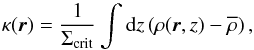 (1)with the convention that the line of sight corresponds to the z-axis and the plane of the sky r vector can be defined by polar coordinates (r,ϕ). The critical density involves distance ratios between a fiducial source at an angular diameter distance Ds, the distance to the lensing mass Dl, and the distance between the lens and the source Dls
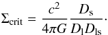 (2)On cosmological scales, the thin lens approximation is generally not valid and the integrated deflections experienced by light rays as they travel from the source to the observer requires numerical treatment, but for most cosmological applications the integration of the deflections along the unperturbed light rays (so-called Born approximation; see e.g. Bartelmann & Schneider 2001) yields a linear integral relation between the convergence κ and the density contrast δ. For a known time-varying1 3D power spectrum Pδ(k,χ), and for a given source plane redshift zs, one can thus write the convergence power spectrum Pκ(ℓ,zs) by means of the Limber approximation (Blandford et al. 1991; Miralda-Escudé 1991; Kaiser 1992; Bartelmann & Schneider 2001; Simon 2007)
 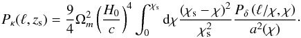 (3)Following early works by Schneider & Bartelmann (1997), we define the aperture multipolar moments of the convergence (projected surface mass density) field κ as
 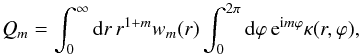 (4)with a radial weight function wm(r) commonly defined on a compact support. Those multipoles aim to quantify possible asymmetries in the mass distribution as probed by gravitational lensing.
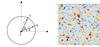 |
Fig. 1 Left-hand panel: this paper aims at describing the angular distribution of a 2D Gaussian field κ around a peak in rz. We therefore consider two points on the annulus at a distance r from the central peak. Their respective Cartesian coordinates are rx = r(cosθ,sinθ) and ry = r(cosθ + ψ,sinθ + ψ). Right-hand panel: example is shown of such a 2D Gaussian random field with a power-law power spectrum with spectral index ns = 0. Peaks of height ν = 3 ± 0.5 are highlighted with black dots. We hereby investigate the polar distribution of the field around such peaks. |
The covariance between multipolar moments can straightforwardly be written as  (5)where Un(ℓ) is the Hankel transform of the radial weight function
  (6)Jm(x) are the first kind Bessel functions and P(k) is the power spectrum of the 2D random field κ.
In a suite of papers (including Gouin et al. 2017, and Gavazzi et al., in prep.), we propose using the full statistics of these multipolar moments around clusters of galaxies. The covariance of the aperture multipolar moments in specific locations of space, such as the vicinity of clusters, becomes  (7)where ⟨ κ(r,ϕ)κ(r′,ϕ′) | clusters ⟩ is a constrained two-point correlation function as we impose a cluster at the origin of the polar coordinate system.
In order to develop a physical intuition of the effect of this cluster constraint on the statistics of the multipolar moments, we propose in this paper to study analytically this observable for a Gaussian random field in which clusters are identified as high peaks. To simplify the problem, we drop the radial weight function and focus on Gaussian random fields smoothed with a Gaussian kernel on a given scale R. In what follows, we investigate the angular distribution of a Gaussian random field around a peak. We therefore need to study the joint statistics of the field in three locations of space: the location of the peak and two arbitrary points on the circle at a distance r away from the central peak. In addition, according to the peak theory originally developed in Bardeen et al. (1986), we need to consider the field and its first and second derivatives at the location of the peak. In Sect. 2.2, we first present the result for the joint PDF of those random variables before computing the resulting multipolar decomposition around a central peak in Sect. 2.6.
2.2. Three-point statistics of the field and its derivatives
 |
Fig. 2 Left-hand panel: number density of minima, saddle points, and peaks compared to the approximation of rare events in units of |

For a given 2D Gaussian field κ (for example, the projected density contrast), we define the moments  (8)From these moments, we use two characteristic lengths R0 = σ0/σ1 and R⋆ = σ1/σ2, as well as the spectral parameter
  (9)We now define the following normalised random variables
  (10)which have unit variance by construction.
In what follows,  denotes the one-point probability density (PDF) and
  designates the joint PDF for the normalised field and its derivatives, X = { x }, Y = { y } , and Z = { z,zi,zij }, at three prescribed comoving locations (rx,ry and rz) separated by a distance r = | rx − rz | = | ry − rz | so that we are considering the density field in two locations, rx and ry on the same infinitely thin shell around the central peak in rz ; see also the left-hand panel of Fig. 1. The right-hand panel of Fig. 1 shows a Gaussian random field and the position of its peaks. This paper aims to investigate the angular matter distribution around those peaks.
For a Gaussian field (in particular cosmic fields at early times or large scales), the joint PDF is a multivariate normal distribution ![Mathematical equation: \begin{equation} {\cal N}(\vec{X},\vec{Y},\vec{Z})= \frac{\exp \left[-\frac{1}{2} \left(\begin{array}{c} \vec{X} \\ \vec{Y} \\ \vec{Z} \\ \end{array} \right)^{\rm T} \cdot \vec{C} ^{-1}\cdot \left(\begin{array}{c} \vec{X} \\ \vec{Y} \\ \vec{Z} \\ \end{array} \right) \right] } {{\rm det}|\mathbf{C}|^{1/2} \left(2\pi\right)^{\rm (6+3d+d^{2})/4 }} \,, \label{eq:defPDF} \end{equation}](/articles/aa/full_html/2017/09/aa30091-16/aa30091-16-eq48.png) (11)where d is the dimension – d = 2 here – and C is the covariance matrix that depends on the separation vectors only because of homogeneity
(11)where d is the dimension – d = 2 here – and C is the covariance matrix that depends on the separation vectors only because of homogeneity  (12)with
  For instance, for a 2D power-law power spectrum with spectral index ns smoothed with a Gaussian filter (r is now the separation in units of the Gaussian smoothing length)
 ![Mathematical equation: \begin{eqnarray} \left\langle xz \right\rangle &=& _1F_1\left(\frac{n_{\rm s}}{2}+1;1;-\frac{r^2}{4}\right)\equiv \xi(r),\\ \left\langle xy \right\rangle &=&\xi(|\vec{r}_{x}-\vec{r}_{y}|=2 r \sin( \psi/2)),\\ \left\langle x\nabla z \right\rangle &=&\frac{\sqrt{n_{\rm s}+2}}{2\sqrt 2} \, _1F_1\left(\frac{n_{\rm s}}{2}+2;2;-\frac{r^2}{4}\right)\mathbf{r},\\ \left\langle xz_{11} \right\rangle &=&-\frac{\gamma}{2} \left[2 \cos^2(\theta +\psi ) \, _1F_1\left(\frac{n_{\rm s}}{2}+2;1;-\frac{r^2}{4}\right)\right.\\ & &\left. -\cos (2 (\theta +\psi )) \, _1F_1\left(\frac{n_{\rm s}}{2}+2;2;-\frac{r^2}{4}\right)\right],\notag\\ \left\langle xz_{12} \right\rangle &=&-\frac{r^{2}\gamma(n_{\rm s}+4)}{32} \sin(2(\theta +\psi )) \, _1F_1\left(\frac{n_{\rm s}}{2}+3;3;-\frac{r^2}{4}\right),\\ \left\langle xz_{22} \right\rangle&=&-\frac{\gamma}{2} \left[2 \sin ^2(\theta +\psi ) \, _1F_1\left(\frac{n_{\rm s}}{2}+2;1;-\frac{r^2}{4}\right)\right.\\ && \left. +\cos (2 (\theta +\psi )) \, _1F_1\left(\frac{n_{\rm s}}{2}+2;2;-\frac{r^2}{4}\right)\right]\cdot\notag \end{eqnarray}](/articles/aa/full_html/2017/09/aa30091-16/aa30091-16-eq55.png) Here
Here  is the confluent hypergeometric function, ξ is the two-point correlation function of the field, and the spectral parameter reads
  . The correlation matrix CYZ is obviously the same as CXZ once ψ has been set to zero.
2.3. Central peak condition
Equation (11) is sufficient to compute the expectation of any quantity involving the fields and its derivatives up to second order in three different locations. This is the case if one wants to implement a peak condition at the rz location. Indeed, following Longuet-Higgins (1957), Adler (1981), Bardeen et al. (1986), this peak constraint reads | detzij | δD(zi)ΘH( − λi), where δD(zi) ≡ δD(z1)δD(z2) is a product of Dirac delta functions, which imposes the gradient to be zero, ΘH( − λi) ≡ ΘH( − λ1)ΘH( − λ2), a Heaviside function forcing the curvatures (equivalently the eigenvalues of the Hessian matrix λi) to be negative. The factor  encodes the volume associated with each peak, in other words the Jacobian, which allows us to go from a smoothed field distribution to the discrete distribution of peaks. The rareness of the peak ν can also be imposed by adding a factor δD(z − ν). We therefore denote npk(Z) the localised density of peaks
  (22)
(22)
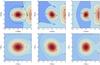 |
Fig. 3 Top panels: expected two-point correlation function ⟨κκ′ | pk⟩ in units of |


The most difficult part in the peak constraint is often to impose the sign of the curvatures and the positivity of the Jacobian, which can prevent us from getting analytical results as is the case for 3D differential peak counts (Gay et al. 2012), or peak-peak correlation functions (as described in Baldauf et al. 2016, in one dimension and Regos & Szalay 1995, in three dimensions), which can only be solved numerically. A standard approximation to keep results analytical is to drop this sign constraint and remove the absolute values of the determinant factor for high contrasts as one expects sufficiently rare critical points to be essentially peaks. If this approximation is very accurate for one-point statistics, it may not be the case for (N> 1) point statistics. For instance, peak-peak correlation functions on small scales are not very well reproduced by this approximation even for large contrasts because the contribution from the other critical points actually dominates at small distance; there is at least one saddle point between two peaks. However, in the context of this work, we impose the peak constraint in one location only and therefore the rare peak approximation is expected to be accurate for  . As an illustration, Fig. 2 shows the Gaussian mean number density of minima, saddle points, and peaks (Longuet-Higgins 1957; Adler 1981, and later generalised to weakly non-Gaussian fields by Pogosyan et al. 2011)
 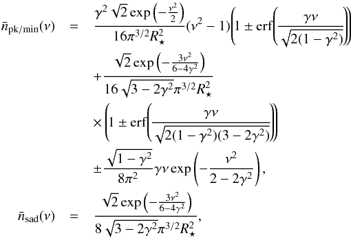 and compares the latter to the high-ν approximation (related to the genus)
  which can be easily computed
 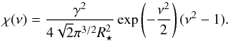 (23)The relative error between the number density of peaks and its high-ν approximation is shown on the right-hand panel of Fig. 2.
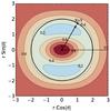 |
Fig. 4 Zero lag annulus correlation function |

2.4. Density correlations on the circle surrounding a central peak with given geometry
The expected product of projected density κ in two locations of space rx and ry such that rx − rz = r(cosθ,sinθ) and ry − rz = r(cos(θ + ψ),sin(θ + ψ)) and given a peak in rz of height ν and curvatures 0 >λ1>λ2 along the first and second coordinates can be analytically computed. For instance for a power-law power spectrum with ns = 0 (and  ), we get
 ![Mathematical equation: \begin{eqnarray} \frac{\left\langle\kappa(r,\theta) \kappa(r,\theta+\psi)|\textrm{pk}\right\rangle}{\sigma_{0}^{2}}&=& \xi(|\vec{r}_{x}-\vec{r}_{y}|)\notag \\ && +\exp\left(-\frac {r^{2}}{2}\right)\left[l_{0}+l_{2}r^{2}+l_{4}r^{4}\right], \end{eqnarray}](/articles/aa/full_html/2017/09/aa30091-16/aa30091-16-eq93.png) (24)where
(24)where ![Mathematical equation: \begin{eqnarray} l_{0}&=& (\nu^{2}-1),\\ l_{2}&=& [\nu^{2}+\sqrt 2\nu I_{1}(1-2 e \cos\psi\cos(2\theta+\psi))-\cos\psi ]/2,\\ l_{4}&=& \left[\nu^{2}-2\cos^{2}\psi+2\sqrt2 \nu I_{1}(1-2 e \cos\psi\cos(2\theta+\psi))\right.\nonumber\\ && \left.+2I_{1}^{2}(1-2 e\cos(2\theta))(1-2 e\cos(2\theta+2\psi))\right]/16, \end{eqnarray}](/articles/aa/full_html/2017/09/aa30091-16/aa30091-16-eq94.png) I1 = λ1 + λ2 is the trace of the density Hessian at the location of the peak, e = (λ2 − λ1) / (2I1) is the ellipticity of the peak and the unconstrained correlation function is
I1 = λ1 + λ2 is the trace of the density Hessian at the location of the peak, e = (λ2 − λ1) / (2I1) is the ellipticity of the peak and the unconstrained correlation function is 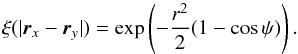 (28)To start with, Fig. 4 shows the zero lag contribution to the annulus correlation function (i.e. when the two points are at the same location on the annulus, ψ = 0) in the frame of the central peak. As expected the amplitude of fluctuations around the peak have an ellipsoidal shape that is more elongated along the smallest curvature λ1 ⋆. This zero-lag annulus correlation is dominated by the square of the mean density profile at small separations and by the fluctuations at larger separations.
Figure 3 then shows the full constrained correlation function on the annulus. We use different orientations of the pair (rx,ry) with regard to the axis of smaller curvature (corresponding to λ1) of the central peak. The orientation of rx is described by the angle θ, which is taken to be 0, π/ 4 and π/ 2 from the left-hand to the right-hand panel. On each plot, the angle between rx and ry, namely ψ, vary between 0 and 2π and the separation to the central peak is described by the value r. We show the result for two different peak heights: the most likely value  (top panels) and a rarer case νr = 3 (bottom panels), which is more relevant to our study. In each case respectively, we fix the peak curvatures to their most likely values
  and λ1r = − 0.94,λ2r = − 1.6, respectively (see Appendix A for a description of the most likely geometry of a peak). As expected, the product of density is larger when the separation vectors are close one to the other and aligned with the major axis of the peak. For the case of a rare peak (bottom panels), the prominence of the peak is obviously larger (increased magnitude and spatial extend of the peak). Conversely, the common peak, ν⋆ occupies a smaller volume and is surrounded by two closer voids and peaks. In what follows, we do not fix the shape of the peak and therefore we marginalise over λ1 and λ2.
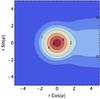 |
Fig. 5 Annulus correlation function ⟨κ(r,θ)κ(r,θ + ψ) | pk(ν)⟩ in units of |
 |
Fig. 6 Multipoles | Qm | 2 | for a central peak with height ν = 2 to 4 as labelled in a Gaussian random field with power spectrum P(k) ∝ k0 smoothed with a Gaussian filter and on the annulus at a distance r = 0.1 R (top left-hand panel), R (top right), and 2 R (bottom left). The dashed line corresponds to the random case in which we do not impose a central peak. The bottom right-hand panel shows the ratio of those multipoles to the random case for r = R. |
2.5. Density correlations around a peak of specified height ν
If one wants to marginalise over the shape of the peak, which means integrating over the eigenvalues λ1 and λ2 in the range λ2<λ1< 0, then the expected product of projected densities on the annulus (the annulus two-point correlation function) becomes 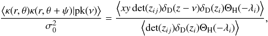 where we marginalise over all variables except ν, which is fixed. Unfortunately, this expression cannot be analytically computed. For sufficiently rare peaks (high ν), we drop the constraint on the sign of the eigenvalues (high critical points are most of the time peaks) and an explicit expression for ⟨κ(r,θ)κ(r,θ + ψ) | pk(ν)⟩ can be obtained
 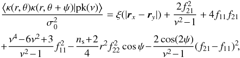 (29)where fij and the unconstrained correlation function ξ( | rx − ry |) are functions of the following Kummer confluent hypergeometric functions
 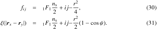 As an illustration, for a power spectrum P(k) ∝ k0, it becomes
 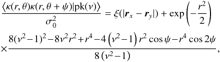 (32)where
 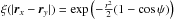 is the unconstrained correlation function on the annulus. The apparent singularity at ν = ± 1 is due to our high ν approximation, which breaks down in this regime as many ν = 1 critical points are not peaks but saddle points. Figure 5 illustrates the behaviour of ⟨κ(r,θ)κ(r,θ + ψ) | pk(ν)⟩ for a central peak with height ν = 3. Similar to the case where the peak geometry is imposed, here the annulus correlation function is larger when the separation vectors are close one to the other and aligned with the major axis of the peak. The isocontours are close to spherical for small separations but become very anisotropic and elongated along the axis ψ = 0 (when the two points overlap) at larger separations.
2.6. Multipoles around a peak of specified height ν
Once the two-point correlation function around a peak – ⟨κ(r,θ)κ(r,θ + ψ) | pk(ν)⟩ – is known, one can compute the corresponding multipolar moments that we define here as 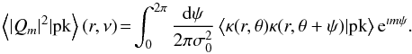 (33)The result is again analytical. As expected, only the first three multipoles are modified by the peak condition,while the rest are unchanged, i.e.,
 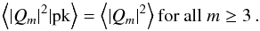 (34)For instance, for P(k) ∝ k0 power spectra, those multipoles read
  where Im are the modified Bessel functions of the first kind. In particular the correction to the monopole (resp. dipole, quadrupole) is maximal for r = 0 (resp.
  , 2). It can easily be checked that the condition of zero gradient only affects the dipole, while the constraint on the peak height changes the monopole and the Hessian modifies both the monopole and quadrupole.
Figure 6 shows the amplitude of the multipoles for various peak heights and separations. There is a significant drop of power in the dipole while the change in the monopole and quadrupole is much less pronounced. The dependence on the peak height is rather small. Those predictions are checked against GRF realisations in Sect. 3.
2.7. Dependence on the slope of the power spectrum
In this work, we have shown results for a power-law power spectrum (ns = 0) but the qualitative conclusions can be shown to be almost independent from the spectral index. To illustrate this property, we computed the multipoles for different slopes of the power spectrum from –1.5 (close to the effective spectral index of the convergence field at cluster scale) to 1 as shown in Fig. 7. The correction to the monopole and dipole are quasi-linearly suppressed when ns increases while the quadruple is constant for a wide range of slopes ns ≲ 1 and shows only a decrease at very low spectral indices. Overall, this shows that the qualitative picture described in this paper does not depend significantly on the slope of the power spectrum. Investigating the effect of its running (i.e the scale-invariance of the slope) is left for future works as no analytical results can be obtained in this case. The study of a more realistic ΛCDM power spectrum in the non-linear regime will be presented elsewhere.
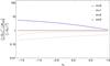 |
Fig. 7 Same as Fig. 6 for central peaks of height ν = 3 and separation r = 1 (in units of the smoothing length) as a function of the spectral index ns. |
3. Comparison with direct measurements in GRF
Let us generate 10 maps of a 20482 GRF with power spectrum P(k) ∝ k0. Each map is then smoothed with a Gaussian kernel on R = 8 pixels. A portion of such a map is shown in the right-hand panel of Fig. 1.
Peaks are then found using the code map2ext (Colombi et al. 2000; Pogosyan et al. 2011): for every pixel a segment of quadratic surface is fit in the tangent plane based on the field values at the pixel of origin and its neighbours. The position of the extremum of this quadratic surface, its height, and its Hessian are computed. The extremum is counted into the tally of the type determined by its Hessian (two negative eigenvalues for peaks) if its position falls within the original pixel. Several additional checks are performed to preclude registering extrema in the neighbouring pixels and to minimise missing extrema due to jumps in the fit parameters as region shifts to the next pixel. This procedure performs with better than 1% accuracy when the map is smoothed with a Gaussian filter whose full width at half maximum exceeds 6 pixels.
The field is then interpolated at 100 equally spaced points on the circle located at r = R around each peak and Fourier transformed. Only the square modulus of the Fourier coefficients are stored. For comparison, a similar procedure is followed to estimate the multipolar decomposition around the same number of random points in the field.
The resulting multipolar decomposition measured in GRF is shown in Fig. 8 for various peak heights and separations. Those measurements are in very good agreement with the theoretical predictions described in Sect. 2.6. The high-ν approximation used to derive the prediction is therefore shown to be very accurate in the regime ν ≥ 2.5. Below this threshold, some departures – in particular in the quadrupole – are seen and would require a numerical integration of the equation with the correct peak curvature constraints.
4. Effect of substructures
In practice, measurements in simulations and observations of the angular distribution of the convergence field around clusters naturally involve two separate scales: the relatively large scale of the cluster and the smaller scale of the convergence field, or the dark matter density field in a N-body simulation, around it. Even if those scales are not identical, they are necessarily highly correlated and the effect described in this paper should persist. To study the effect of substructures, we redo the analysis but introduce two different smoothing lengths, one R1 for the field z at the location of the peak and one R2 at the location of the annulus. In this section only, we denote R = R2/R1 ≤ 1 as the corresponding (dimensionless) ratio. The same formalism as described above applies but all the coefficients of the covariance matrix are changed. Let us first redefine the random variables as  where the factors σi are the respective variances of the field, gradient, and Laplacian smoothed on scale R1. With this definition, one can easily recompute the coefficients of the covariance matrix. For instance,
 ![Mathematical equation: \begin{eqnarray} \left\langle xz \right\rangle&=&\left\langle yz \right\rangle=\beta^{-n_{\rm s}-2}\, _1F_1\left(\frac{n_{\rm s}}{2}+1;1;-\frac{r^2}{4\beta^{2}}\right),\\ \left\langle xy \right\rangle&=&R^{-\frac {n_{\rm s}+2} 2}\, _1F_1\left(\frac{n_{\rm s}}{2}+1;1;-\frac{r^2}{2R^{2}}(1-\cos\psi)\right),\\ \left\langle xz_{22} \right\rangle&=&-\frac{\gamma}{2} \beta^{-n_{\rm s}-4}\left[2 \sin ^2(\theta +\psi ) \, _1F_1\left(\frac{n_{\rm s}}{2}+2;1;-\frac{r^2}{4\beta^{2}}\right)\right.\nonumber\\ & & \left.+\cos (2 (\theta +\psi )) \, _1F_1\left(\frac{n_{\rm s}}{2}+2;2;-\frac{r^2}{4\beta^{2}}\right)\right], \end{eqnarray}](/articles/aa/full_html/2017/09/aa30091-16/aa30091-16-eq145.png) where the separation r is again a dimensionless quantity (expressed in units of R1) and β is the dimensionless quadratic mean of the two smoothing lengths
where the separation r is again a dimensionless quantity (expressed in units of R1) and β is the dimensionless quadratic mean of the two smoothing lengths  (44)which ranges from
  , when R2 goes to zero, to 1, when the two smoothing scales are equal R2 = R1.
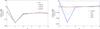 |
Fig. 8 Left-hand panel: same as the bottom right-hand panel of Fig. 6 for measurements in 10 realisations of a 20482 2D GRF smoothed with a Gaussian filter on 8 pixels. The height of the peaks are binned as labelled and the separation considered here is r = R = 8 pixels. Right-hand panel: same as left-hand panel when we vary the separation r instead of the peak height, which is set to ν = 3 here. We overplotted the theoretical predictions with dashed lines that are almost indistinguishable from the measurements. |
An analytical solution for the mean amplitude of the multipoles of the field around a central peak can again be computed. For the same example of a power-law power spectrum P(k) ∝ k0, those multipoles read 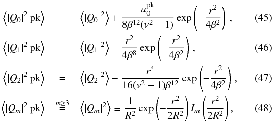 where Im are the modified Bessel functions of the first kind and
 ![Mathematical equation: \begin{eqnarray*} {a_{0}^{\rm pk}}&=&r^{4}-8\beta^{2}\left[1+\beta^{2}(\nu^{2}-1)\right]r^{2}\nonumber\\ && +8\beta^{4}\left[2+4\beta^{2}(\nu^{2}-1)+\beta^{4}(\nu^{4}-6\nu^{2}+3)\right]. \end{eqnarray*}](/articles/aa/full_html/2017/09/aa30091-16/aa30091-16-eq152.png) The limit R = β = 1 trivially reduces to the former Eqs. (35)–(38).
The limit R = β = 1 trivially reduces to the former Eqs. (35)–(38).
Those small-scale multipoles are shown in Fig. 9 for R = 1 / 100 to R = 1. The multiscale approach described in this section does not modify the m> 2 multipoles. As expected, the correction due to the peak decreases when R goes to 0 as the scales decorrelate. In addition, we expect that non-linearities and corrections beyond the Hessian change the power of higher order multipoles.
5. Beyond the thin shell approximation
The effect of the radial weight function in Eq. (7) can be studied by relaxing the assumption that rx and ry are on a same infinitely thin shell around the central peak in rz. Let us therefore consider the general setting for which rx is at a distance r from the central peak and ry at a distance r′. In this case, the constrained two-point correlation function reads 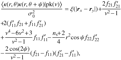 (49)where f, f′, and the unconstrained correlation function ξ( | rx − ry |) are functions of the following Kummer confluent hypergeometric functions
 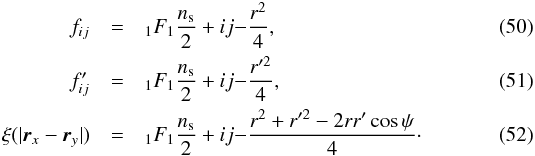 It can easily be checked that Eq. (49) trivially reduces to Eq. (29) when r′ = r. As an illustration, for a power-law power spectrum P(k) ∝ k0, the correction to the unconstrained correlation functionξ( | rx − ry |) reads
 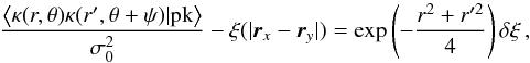 (53)with
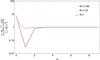 |
Fig. 9 Same as the bottom right-hand panel of Fig. 6 when the field is smoothed at two different scales whose ratio R goes from 1/100 to 1. |
From Eq. (49), one can now easily compute the statistics of the multipoles including the radial weight function wn(r) that appears in Eq. (7). We find again that only the amplitude of the first three multipoles are affected by the peak constraint  where
where  stands for the following 2D radial integral
 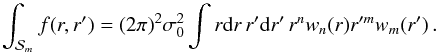 (58)Figure 10 shows the resulting multipoles for a radial weight function defined following Schneider & Bartelmann (1997) as
 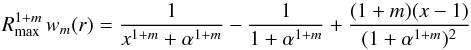 (59)over the range x = r/Rmax ∈ [ α,1 ] and zero elsewhere (which was found to be optimal for an isothermal mass distribution). The qualitative picture does not change; the most affected multipole is the dipole whose power is significantly reduced by the peak constraint, the monopole and quadrupole are slightly affected in a ν-dependent way, and all other coefficients are unaffected.
 |
Fig. 10 Same as the bottom right-hand panel of Fig. 6 when we apply a radial weight function defined by Eq. (59), where Rmax equals the smoothing length and α = 0.5, which means that the minimum radius considered is half the smoothing length. |
 |
Fig. 11 Slice through the fields nstep = 0,1,2, and 3 obtained by a Zeldovich displacement of an initial GRF. We measure the multipolar moments around all points of height ν> 2 in those maps. |
6. A non-linear theory of harmonic power spectra
In this section, we study the weakly non-linear evolution of the multipolar moments. We therefore no longer assume that the PDF is Gaussian  . Instead, we expand the PDF around a Gaussian by means of the so-called Gram-Charlier expansion (Cramér 1946; Pogosyan et al. 2009a). For simplicity, we restrict ourselves to the case in which we only impose the height of the cluster but not the rest of the peak condition (no zero gradient or constraint on the eigenvalues of the Hessian). We show that this effect dominates the high multipoles.
6.1. The Gram Charlier expansion
The Gaussian PDF has zero means and covariance matrix ![Mathematical equation: \begin{equation} \mathbf{C}=\left( \begin{array}{cccccc} 1 & b&a \\[2mm] b & 1 &a \\[2mm] a & a&1 \end{array} \right), \end{equation}](/articles/aa/full_html/2017/09/aa30091-16/aa30091-16-eq177.png) (60)with a = ξ(r) and b = ξ(2rsin(ψ/ 2)).
(60)with a = ξ(r) and b = ξ(2rsin(ψ/ 2)).
We first diagonalise this matrix and use a new set of variables (u,v,z), where 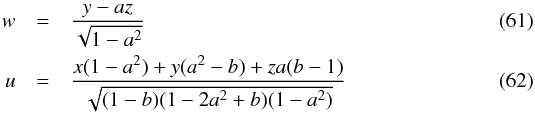 so that
  (63)with N a normal distribution of zero mean and unit variance.
Following Gay et al. (2012), Codis et al. (2013), we then use a Gram-Charlier expansion of the PDF ![Mathematical equation: \begin{eqnarray*} {\cal P}(u,w,z)={G}(u,w,z)\left[1+\!\!\!\sum_{i+j+k=3}^{\infty}\frac{H_{i}(u)H_{j}(w)H_{k}(z)}{i!\,j!\,k!}\left\langle u^{i} w^{j} z^{k}\right\rangle_{\rm GC}\right], \end{eqnarray*}](/articles/aa/full_html/2017/09/aa30091-16/aa30091-16-eq183.png) where Hi represent probabilistic Hermite polynomials and the Gram-Charlier coefficients are given by
where Hi represent probabilistic Hermite polynomials and the Gram-Charlier coefficients are given by  (64)Once the joint PDF is known, we can compute the annulus two-point correlation function ⟨xy | z = ν⟩ as
 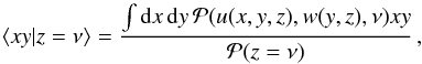 (65)which can be rewritten
 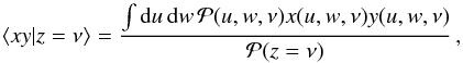 (66)where xy is a polynomial of u and w
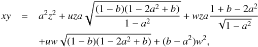 (67)which is the sum of four terms proportional respectively to H0(u)H0(w), H1(u)H0(w), H0(u)H1(w), H1(u)H1(w) and H0(u)(H2(w) + H0(w)) as H0(x) = 1, H1(x) = x and H2(x) = x2 − 1, respectively. Using the property of orthogonality of Hermite polynomials, it is then easy to compute Eq. (66)so that eventually
 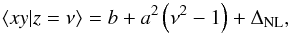 (68)where the non-linear contribution reads
 ![Mathematical equation: \begin{eqnarray*} \Delta_{\rm NL} = \frac{\sum_{k=1}^{\infty}\!\frac{H_{k}(\nu)}{k!}\!\left\langle H_{k}(z)\!\left[\!2a\nu(x\!-\!az)\!+\!xy\!-\!b\!-\!2azx\!+\!a^{2}z^{2}+a^{2}\right]\right\rangle}{1+\!\sum_{k=3}^{\infty}\frac{H_{k}(\nu)}{k!}\left\langle z^{k}\right\rangle_{\rm GC}}, \end{eqnarray*}](/articles/aa/full_html/2017/09/aa30091-16/aa30091-16-eq202.png) which, at first order in σ0, the amplitude of fluctuations, is given by2
which, at first order in σ0, the amplitude of fluctuations, is given by2 In terms of multipoles, it means that for m> 0, we get a non-linear bias given by
 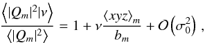 (69)where the subscript m refers to the associated multipole of order m. The multipoles near a high density cluster are therefore biased compared to random locations; this bias is proportional to the height ν with a proportionality coefficient related to the ratio between the isosceles three-point function ⟨xyz⟩ and the two-point correlation function of its base b = ⟨xy⟩ = ξ(2rsin(ψ/ 2)). The all-order expression is also easily obtained once it is realised that the only terms that depend on the angle ψ are b and the cumulants involving the product xy
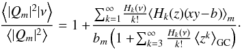 (70)The monopole is also easy to compute
 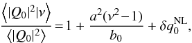 (71)where the first order non-linear correction reads
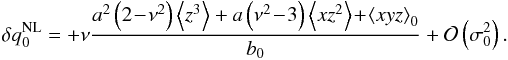
6.2. Comparison with simulations
To test the m> 0 prediction, we have generated various GRF and displaced the density field following a Zeldovich displacement with different time steps denoted nstep = 0,1,2, and 3 (from Gaussian to more evolved fields). In practice, we compute the displacement field as the gradient of the gravitational potential by FFT and we multiply by a constant times nstep. We then move the mass in each pixel according to this displacement and distribute it to the eight closest pixels. Those fields are illustrated in Fig. 11. We measure the multipoles around field point of height ν> 2 together with the mean height of those peaks (resp.  ) and the multipolar decomposition of the bispectrum ⟨xyz⟩m. The result is shown in Fig. 12 and shows a fair agreement of the m> 0 multipoles with the prediction given in Eq. (69).
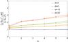 |
Fig. 12 Ratio between the multipolar moments at a distance r = 8 pixels from a field point of height ν> 2 compared to random locations, for a GRF displaced following the Zeldovich approximation for different time steps between 0 and 20 as labelled and smoothed over 3 pixels. The solid line is the measurements and the dashed line is the prediction for m> 0 given by Eq. (69). |
7. Conclusions
We have computed the statistics of the multipolar moments around a peak for a generic 2D Gaussian field as a proxy for the azimuthal distribution of matter around clusters seen by weak gravitational lensing experiments. For rare enough peaks ( ), all results are completely analytical. It is shown that only the monopole, dipole, and quadrupole are affected by the central peak while higher order multipoles are essentially left unchanged by the peak constraint. Overall, the dominant effect we find is a significant drop in the dipole coefficient as expected from the zero gradient condition. Substructures in the Gaussian field and the addition of a radial weighting function do not change this qualitative picture.
This feature in the dipole can also be detected in numerical simulations of structure formation as will be shown in a forthcoming paper (Gouin et al. 2017). We anticipate that higher order corrections will also emerge from the non-linear evolution of the density field in the vicinity of peaks beyond the Gaussian picture described here, and also from a possible departure from the peak model itself which, as we showed in this paper, boils down to modifying the power in the monopole, dipole, and quadrupole only. As an illustration, we computed the non-linear bias of the multipolar moments due to the height of the cluster. This bias is proportional to the height ν and to the variance of the field σ by means of the rescaled bispectrum. This approach based on the statistics of multipolar moments in the convergence field around clusters will soon be applied to data (Gavazzi et al., in prep.).
Extensions of this analytical work in the future might include i) an investigation of the accuracy of the large ν approximation and a precise numerical integration in the regime of intermediate contrasts where this approximation breaks down; and ii) a study of the effect of the scale-dependence of the power spectrum.
Where time variation is captured by an explicit dependence on comoving distance χ.
An easy way to get this expression is to only keep Gram-Charlier coefficients  for which i + j + k = 3, which were shown to be equivalent to cumulants and correspond exactly to the first-order correction that is proportional to σ0 (Gay et al. 2012).
Acknowledgments
This work is partially supported by the grants ANR-13-BS05-0005 of the French Agence Nationale de la Recherche. This work has made use of the Horizon cluster on which the GRF maps were generated, hosted by the Institut d’Astrophysique de Paris. We warmly thank D. Pogosyan for insightful discussions, his careful reading of the manuscript, and for providing us with his code map2ext to detect extrema in 2D maps. We also thank S. Rouberol for running the Horizon cluster for us and D. Munro for freely distributing his Yorick programming language and opengl interface (available at yorick.sourceforge.net).
References
- Adler, R. J. 1981, The Geometry of Random Fields (Chichester: Wiley) [Google Scholar]
- Aragón-Calvo, M. A., van de Weygaert, R., Jones, B. J. T., & van der Hulst, J. M. 2007, ApJ, 655, L5 [NASA ADS] [CrossRef] [Google Scholar]
- Aragon-Calvo, M. A., & Yang, L. F. 2014, MNRAS, 440, L46 [NASA ADS] [CrossRef] [Google Scholar]
- Aubert, D., & Pichon, C. 2007, MNRAS, 374, 877 [NASA ADS] [CrossRef] [Google Scholar]
- Aubert, D., Pichon, C., & Colombi, S. 2004, MNRAS, 352, 376 [NASA ADS] [CrossRef] [Google Scholar]
- Bailin, J., & Steinmetz, M. 2005, ApJ, 627, 647 [Google Scholar]
- Baldauf, T., Codis, S., Desjacques, V., & Pichon, C. 2016, MNRAS, 456, 3985 [NASA ADS] [CrossRef] [Google Scholar]
- Bardeen, J. M., Bond, J. R., Kaiser, N., & Szalay, A. S. 1986, ApJ, 304, 15 [NASA ADS] [CrossRef] [Google Scholar]
- Bartelmann, M., & Schneider, P. 2001, Phys. Rep., 340, 291 [NASA ADS] [CrossRef] [Google Scholar]
- Blandford, R. D., Saust, A. B., Brainerd, T. G., & Villumsen, J. V. 1991, MNRAS, 251, 600 [NASA ADS] [Google Scholar]
- Bond, J. R., & Myers, S. T. 1996, ApJS, 103, 1 [NASA ADS] [CrossRef] [Google Scholar]
- Bond, J. R., Kofman, L., & Pogosyan, D. 1996, Nature, 380, 603 [NASA ADS] [CrossRef] [Google Scholar]
- Brunino, R., Trujillo, I., Pearce, F. R., & Thomas, P. A. 2007, MNRAS, 375, 184 [NASA ADS] [CrossRef] [Google Scholar]
- Codis, S., Pichon, C., Devriendt, J., et al. 2012, MNRAS, 427, 3320 [NASA ADS] [CrossRef] [Google Scholar]
- Codis, S., Pichon, C., Pogosyan, D., Bernardeau, F., & Matsubara, T. 2013, MNRAS, 435, 531 [NASA ADS] [CrossRef] [Google Scholar]
- Codis, S., Pichon, C., & Pogosyan, D. 2015, MNRAS, 452, 3369 [Google Scholar]
- Colombi, S., Pogosyan, D., & Souradeep, T. 2000, Phys. Rev. Lett., 85, 5515 [NASA ADS] [CrossRef] [Google Scholar]
- Cramér, H. 1946, Mathematical Methods of Statistics (Princeton Univ. Press) [Google Scholar]
- Davé, R., Cen, R., Ostriker, J. P., et al. 2001, ApJ, 552, 473 [NASA ADS] [CrossRef] [Google Scholar]
- Dietrich, J. P., Schneider, P., Clowe, D., Romano-Díaz, E., & Kerp, J. 2005, A&A, 440, 453 [NASA ADS] [CrossRef] [EDP Sciences] [Google Scholar]
- Doroshkevich, A. G. 1970, Astrophysics, 6, 320 [NASA ADS] [CrossRef] [Google Scholar]
- Dubois, Y., Pichon, C., Welker, C., et al. 2014, MNRAS, 444, 1453 [NASA ADS] [CrossRef] [Google Scholar]
- Fukugita, M., Hogan, C. J., & Peebles, P. J. E. 1998, ApJ, 503, 518 [NASA ADS] [CrossRef] [Google Scholar]
- Gay, C., Pichon, C., Le Borgne, D., et al. 2010, MNRAS, 404, 1801 [NASA ADS] [Google Scholar]
- Gay, C., Pichon, C., & Pogosyan, D. 2012, Phys. Rev. D, 85, 023011 [NASA ADS] [CrossRef] [Google Scholar]
- Gouin, C., Gavazzi, R., Codis, S., et al. 2017, A&A, 605, A27 [NASA ADS] [CrossRef] [EDP Sciences] [Google Scholar]
- Guzzo, L., Strauss, M. A., Fisher, K. B., Giovanelli, R., & Haynes, M. P. 1997, ApJ, 489, 37 [NASA ADS] [CrossRef] [Google Scholar]
- Hahn, O., Porciani, C., Carollo, C. M., & Dekel, A. 2007, MNRAS, 375, 489 [NASA ADS] [CrossRef] [Google Scholar]
- Hahn, O., Teyssier, R., & Carollo, C. M. 2010, MNRAS, 405, 274 [NASA ADS] [Google Scholar]
- Kaiser, N. 1984, ApJ, 284, L9 [NASA ADS] [CrossRef] [Google Scholar]
- Kaiser, N. 1992, ApJ, 388, 272 [NASA ADS] [CrossRef] [Google Scholar]
- Klypin, A., & Shandarin, S. F. 1993, ApJ, 413, 48 [NASA ADS] [CrossRef] [Google Scholar]
- Kovač, K., Lilly, S. J., Knobel, C., et al. 2014, MNRAS, 438, 717 [NASA ADS] [CrossRef] [Google Scholar]
- Longuet-Higgins, M. S. 1957, Phil. Trans. R. Soc. London Ser. A, 249, 321 [NASA ADS] [CrossRef] [Google Scholar]
- Ludlow, A. D., & Porciani, C. 2011, MNRAS, 413, 1961 [NASA ADS] [CrossRef] [Google Scholar]
- Martinet, N., Clowe, D., Durret, F., et al. 2016, A&A, 590, A69 [NASA ADS] [CrossRef] [EDP Sciences] [Google Scholar]
- Mead, J. M. G., King, L. J., & McCarthy, I. G. 2010, MNRAS, 401, 2257 [NASA ADS] [CrossRef] [Google Scholar]
- Metuki, O., Libeskind, N. I., Hoffman, Y., Crain, R. A., & Theuns, T. 2015, MNRAS, 446, 1458 [NASA ADS] [CrossRef] [Google Scholar]
- Miralda-Escudé, J. 1991, ApJ, 380, 1 [NASA ADS] [CrossRef] [Google Scholar]
- Navarro, J. F., Abadi, M. G., & Steinmetz, M. 2004, ApJ, 613, L41 [NASA ADS] [CrossRef] [Google Scholar]
- Oemler, Jr., A. 1974, ApJ, 194, 1 [NASA ADS] [CrossRef] [Google Scholar]
- Paranjape, A., & Sheth, R. K. 2012, MNRAS, 426, 2789 [NASA ADS] [CrossRef] [Google Scholar]
- Paz, D. J., Stasyszyn, F., & Padilla, N. D. 2008, MNRAS, 389, 1127 [NASA ADS] [CrossRef] [Google Scholar]
- Persic, M., & Salucci, P. 1992, MNRAS, 258, 14 [NASA ADS] [CrossRef] [Google Scholar]
- Pogosyan, D., Gay, C., & Pichon, C. 2009a, Phys. Rev. D, 80, 081301 [NASA ADS] [CrossRef] [Google Scholar]
- Pogosyan, D., Pichon, C., Gay, C., et al. 2009b, MNRAS, 396, 635 [CrossRef] [Google Scholar]
- Pogosyan, D., Pichon, C., & Gay, C. 2011, Phys. Rev. D, 84, 083510 [NASA ADS] [CrossRef] [Google Scholar]
- Regos, E., & Szalay, A. S. 1995, MNRAS, 272, 447 [NASA ADS] [CrossRef] [Google Scholar]
- Schneider, P., & Bartelmann, M. 1997, MNRAS, 286, 696 [NASA ADS] [CrossRef] [Google Scholar]
- Shull, J. M., Smith, B. D., & Danforth, C. W. 2012, ApJ, 759, 23 [NASA ADS] [CrossRef] [Google Scholar]
- Simon, P. 2007, A&A, 473, 711 [NASA ADS] [CrossRef] [EDP Sciences] [Google Scholar]
- Sousbie, T., Pichon, C., Colombi, S., & Pogosyan, D. 2008, MNRAS, 383, 1655 [Google Scholar]
- Tempel, E., & Libeskind, N. I. 2013, ApJ, 775, L42 [NASA ADS] [CrossRef] [Google Scholar]
Appendix A: Typical peak geometry
The typical geometry of a Gaussian peak in two dimensions can easily be computed. Starting from the Gaussian joint PDF of the field value ν and local curvatures λ1>λ2 (Doroshkevich 1970; Pogosyan et al. 2009b) 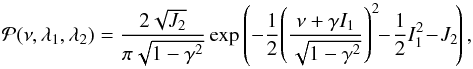 (A.1)where I1 = λ1 + λ2 and J2 = (λ1 − λ2)2, one can show that the PDF for a peak to have height ν and geometry 0 >λ1>λ2 reads (Bardeen et al. 1986; Codis et al. 2015)
  (A.2)It has to be emphasised that here we do impose exactly the peak constraint given by Eq. (22). The most likely value of the peak height and curvatures is therefore given by
  ,
, 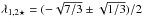 , which corresponds to an ellipticity
  .
.
If ν is fixed, for example to a rare value νr = 3, the maximum of the PDF given by Eq. (A.2) is changed to λ1r = − 0.94 and λ2r = − 1.6 so that the ellipticity of the peak is given by er = 0.13, independently from the spectral parameter γ. The evolution of the most likely peak curvatures as a function of height is shown in Fig. A.1. In particular, this illustrates the well-known result that high peaks are increasingly spherical.
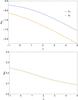 |
Fig. A.1 Most likely peak curvatures as a function of the peak height ν (top panel) and the corresponding most likely peak ellipticity (bottom panel). These results do not depend on the spectral index. |
All Figures
|
Fig. 1 Left-hand panel: this paper aims at describing the angular distribution of a 2D Gaussian field κ around a peak in rz. We therefore consider two points on the annulus at a distance r from the central peak. Their respective Cartesian coordinates are rx = r(cosθ,sinθ) and ry = r(cosθ + ψ,sinθ + ψ). Right-hand panel: example is shown of such a 2D Gaussian random field with a power-law power spectrum with spectral index ns = 0. Peaks of height ν = 3 ± 0.5 are highlighted with black dots. We hereby investigate the polar distribution of the field around such peaks. |
| In the text | |
|
Fig. 2 Left-hand panel: number density of minima, saddle points, and peaks compared to the approximation of rare events in units of |
| In the text | |
|
Fig. 3 Top panels: expected two-point correlation function ⟨κκ′ | pk⟩ in units of |
| In the text | |
|
Fig. 4 Zero lag annulus correlation function |
| In the text | |
|
Fig. 5 Annulus correlation function ⟨κ(r,θ)κ(r,θ + ψ) | pk(ν)⟩ in units of |
| In the text | |
|
Fig. 6 Multipoles | Qm | 2 | for a central peak with height ν = 2 to 4 as labelled in a Gaussian random field with power spectrum P(k) ∝ k0 smoothed with a Gaussian filter and on the annulus at a distance r = 0.1 R (top left-hand panel), R (top right), and 2 R (bottom left). The dashed line corresponds to the random case in which we do not impose a central peak. The bottom right-hand panel shows the ratio of those multipoles to the random case for r = R. |
| In the text | |
|
Fig. 7 Same as Fig. 6 for central peaks of height ν = 3 and separation r = 1 (in units of the smoothing length) as a function of the spectral index ns. |
| In the text | |
|
Fig. 8 Left-hand panel: same as the bottom right-hand panel of Fig. 6 for measurements in 10 realisations of a 20482 2D GRF smoothed with a Gaussian filter on 8 pixels. The height of the peaks are binned as labelled and the separation considered here is r = R = 8 pixels. Right-hand panel: same as left-hand panel when we vary the separation r instead of the peak height, which is set to ν = 3 here. We overplotted the theoretical predictions with dashed lines that are almost indistinguishable from the measurements. |
| In the text | |
|
Fig. 9 Same as the bottom right-hand panel of Fig. 6 when the field is smoothed at two different scales whose ratio R goes from 1/100 to 1. |
| In the text | |
|
Fig. 10 Same as the bottom right-hand panel of Fig. 6 when we apply a radial weight function defined by Eq. (59), where Rmax equals the smoothing length and α = 0.5, which means that the minimum radius considered is half the smoothing length. |
| In the text | |
|
Fig. 11 Slice through the fields nstep = 0,1,2, and 3 obtained by a Zeldovich displacement of an initial GRF. We measure the multipolar moments around all points of height ν> 2 in those maps. |
| In the text | |
|
Fig. 12 Ratio between the multipolar moments at a distance r = 8 pixels from a field point of height ν> 2 compared to random locations, for a GRF displaced following the Zeldovich approximation for different time steps between 0 and 20 as labelled and smoothed over 3 pixels. The solid line is the measurements and the dashed line is the prediction for m> 0 given by Eq. (69). |
| In the text | |
|
Fig. A.1 Most likely peak curvatures as a function of the peak height ν (top panel) and the corresponding most likely peak ellipticity (bottom panel). These results do not depend on the spectral index. |
| In the text | |
Current usage metrics show cumulative count of Article Views (full-text article views including HTML views, PDF and ePub downloads, according to the available data) and Abstracts Views on Vision4Press platform.
Data correspond to usage on the plateform after 2015. The current usage metrics is available 48-96 hours after online publication and is updated daily on week days.
Initial download of the metrics may take a while.