© ESO, 2017

1. Introduction

X-ray spectra of astrophysical sources are often characterised by relatively low numbers of counts per spectral bin. In the early days, spectral models were often tested using χ²-statistics. The goodness of fit is expressed as ${\mathit{\chi }}^{\mathrm{2}}\mathrm{=}\sum _{\mathit{i}\mathrm{=}\mathrm{1}}^{\mathit{n}}\frac{\mathrm{(}{\mathit{N}}_{\mathit{i}}\mathrm{-}{\mathit{s}}_{\mathit{i}}{\mathrm{)}}^{\mathrm{2}}}{{\mathit{\sigma }}_{\mathit{i}}^{\mathrm{2}}}\mathit{,}$(1)where the summation over i is over all n bins of the spectrum, N_i is the observed number of counts, s_i is the expected number of counts for the tested model, and ${\mathit{\sigma }}_{\mathit{i}}^{\mathrm{2}}\mathrm{=}{\mathit{s}}_{\mathit{i}}$ for Poissonian statistics. There are three important remarks to make here.

First, both the model s_i and the observed spectrum N_i should include the source plus background counts to properly use Poissonian statistics.

Secondly, minimisation of χ² to obtain the best-fit parameters of the model is easier when ${\mathit{\sigma }}_{\mathit{i}}^{\mathrm{2}}$ is approximated by N_i, which is a reasonable approximation when N_i is large and the Poissonian distribution approaches a normal distribution, but it fails for small N_i, which can be easily seen by putting σ_i = 0 in (1). This method leads to biased results, even for higher count rates (e.g. Nousek & Shue 1989; Mighell 1999). There are methods to compensate for this, however all of these have some drawbacks. For example the Gehrels (1986) approximation for N_i in the denominator of (1) causes problems when spectra are rebinned. Using ${\mathit{\sigma }}_{\mathit{i}}^{\mathrm{2}}\mathrm{=}{\mathit{s}}_{\mathit{i}}$ (e.g. Wheaton et al. 1995) properly requires multiple passes through the minimisation procedure, updating ${\mathit{\sigma }}_{\mathit{i}}^{\mathrm{2}}$ at each step and sometimes leading to oscillatory behaviour.

Finally, it is often common practice in case of small N_i to rebin the spectra to at least 25 counts per bin or a similar sized number. This has the risk of washing out spectral details.

It has been pointed out by Cash (1979) that $\begin{array}{c}\mathrm{˜}\\ \mathit{C}\end{array}\mathrm{=}\mathrm{2}\sum _{\mathit{i}\mathrm{=}\mathrm{1}}^{\mathit{n}}{\mathit{s}}_{\mathit{i}}\mathrm{-}{\mathit{N}}_{\mathit{i}}\ln \mathrm{\left(}{\mathit{s}}_{\mathit{i}}\mathrm{\right)}$(2)is a much better statistic and can be applied to bins with a small number of counts without any bias in the derived parameters. Also, this statistic can be used to derive uncertainty ranges on the parameters of the model. It is often stated that the Cash-statistic $\begin{array}{c}{\mathrm{˜}}_{}\\ \mathit{C}\end{array}$ cannot be used to measure the goodness of the fit using a quantity corresponding for instance to the reduced ${\mathit{\chi }}_{\mathit{r}}^{\mathrm{2}}\mathrm{\equiv }{\mathit{\chi }}^{\mathrm{2}}\mathit{/}\mathrm{(}\mathit{n}\mathrm{-}\mathit{p}\mathrm{)}\mathit{,}$ where p is the number of free parameters. For example, Nousek & Shue (1989) noted, “The principal disadvantage of the C statistic is that there is no value corresponding to the reduced χ² value with which we can measure the goodness of the fit”, and Humphrey et al. (2009) wrote, “Since the absolute value of the C-statistic cannot be directly interpreted as a goodness-of-fit indicator observers typically prefer instead to minimize the better-known χ²-fit statistic”. Maybe because of this many X-ray astronomers keep using χ²-statistics, even in cases where the approximation breaks down or leads to biased parameters.

In this paper, I present calculations that can be used to evaluate the expected value for C and its root-mean-squared (rms) deviation to assess the goodness of fit of a spectral model derived from a best fit to the observed spectrum.

I use a modification of the original Cash-statistic that has been attributed to Castor and is implemented in current fitting packages such as XSPEC (Arnaud 1996), SHERPA (Freeman et al. 2001), and SPEX (Kaastra et al. 1996). This modified C-statistic, designated here as cstat, is defined as $\mathit{C}\mathrm{=}\mathrm{2}\sum _{\mathit{i}\mathrm{=}\mathrm{1}}^{\mathit{n}}{\mathit{s}}_{\mathit{i}}\mathrm{-}{\mathit{N}}_{\mathit{i}}\mathrm{+}{\mathit{N}}_{\mathit{i}}\ln \mathrm{(}{\mathit{N}}_{\mathit{i}}\mathit{/}{\mathit{s}}_{\mathit{i}}\mathrm{)}$(3)and has similar properties as the original Cash statistic, but in addition it can be used to assign a goodness-of-fit measure to the fit. For a spectrum with many counts per bin C → χ², but where the predicted number of counts per bin is small, the expected value for C can be substantially smaller than the number of bins n.

2. Expected value of C and its variance

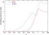Fig. 1 Expected value of the contribution per bin to C, and its rms uncertainty as a function of the mean expected number of counts μ.

The expected contribution C_e,i to the total C from any individual bin i and its variance C_v,i are given by $\begin{array}{ccc}& & \\ & & {\mathit{S}}_{\mathrm{v}\mathit{,i}}\mathrm{=}\mathrm{4}\sum _{\mathit{k}\mathrm{=}\mathrm{0}}^{\mathrm{\infty }}{\mathit{P}}_{\mathit{k}}\mathrm{\left(}\mathit{\mu }\mathrm{\right)}{\left[\mathit{\mu }\mathrm{-}\mathit{k}\mathrm{+}\mathit{k}\ln \mathrm{(}\mathit{k}\mathit{/}\mathit{\mu }\mathrm{)}\right]}^{\mathrm{2}}\mathit{,}\\ & & \end{array}$with P_k(μ) the Poisson distribution ${\mathit{P}}_{\mathit{k}}\mathrm{\left(}\mathit{\mu }\mathrm{\right)}\mathrm{=}{\mathrm{e}}^{\mathrm{-}\mathit{\mu }}{\mathit{\mu }}^{\mathit{k}}\mathit{/}\mathit{k}\mathrm{!}$(7)and μ the expected number of counts in the relevant bin. We show C_e,i and $\sqrt{{\mathit{C}}_{\mathrm{v}\mathit{,i}}}$ in Fig. 1.

The above equations hold for a single bin. For the full spectrum, the expected values C_e,i and variances C_v,i can be simply added over all bins i, yielding the expected value and variance for the full spectrum.

While the above procedure yields the exact expected mean value and variance for C, in general this does not mean that C has a Gaussian distribution with that mean and variance. A Gaussian distribution occurs when each bin, or most bins, i, have enough counts such that the distribution of C_i becomes asymptotically Gaussian, or for lower numbers of counts when the number of spectral bins is large enough. In the latter case we can use the central limit theorem, which states that when independent random variables are added, their sum tends towards a normal distribution even if the original variables themselves are not normally distributed.

In the above case, acceptable spectral models typically have ΣC_e,i(μ_i)−f[ΣC_v,i(μ_i)]^0.5<C< ΣC_e,i(μ_i) + f[ΣC_v,i(μ_i)]^0.5 with f a factor of order unity corresponding to the required significance level, for instance f = 1 for 68% confidence.

When these above conditions are not met, i.e. for low number of counts or low number of spectral bins, the distribution of C is not Gaussian. In that case the higher order moments of the distribution of C can be calculated analogous to (4) and (6). These can be used in principle to build the distribution of C. This can be a cumbersome task, however, and alternatively, using the best-fit model, one may test it simply by running multiple simulations of the spectrum to obtain an empirical distribution of C from which the goodness of fit can be estimated.

Fortunately, in most practical cases using the total mean and variance of C with a simple Gaussian approximation is accurate enough to assess the goodness of fit. We illustrate this with two practical examples in Sect. 3.

We implemented the above approach in the SPEX package¹ (Kaastra et al. 1996). To help the user to see if a C-value corresponds to an acceptable fit, SPEX gives, after spectral fitting, the expected value of C and its rms spread, based on the best-fit model. Both quantities are simply determined by adding the expected contributions and their variances over all bins.

3. Simple approximations for the expected value and variance of C

We obtained simple approximations to the infinite series involved in (4) and (6), with relative errors better than 2.2 × 10^-4 for C_e and better than 1.6 × 10^-4 for C_v, as follows: $\begin{array}{ccc}\mathrm{0}\mathrm{\le }\mathit{\mu }\mathrm{\le }\mathrm{0.5}\mathrm{:}& {\mathit{C}}_{\mathrm{e}}& \mathrm{=}\mathrm{-}\mathrm{0.25}{\mathit{\mu }}^{\mathrm{3}}\mathrm{+}\mathrm{1.38}{\mathit{\mu }}^{\mathrm{2}}\mathrm{-}\mathrm{2}\mathit{\mu }\ln \mathit{\mu }\\ \mathrm{0.5}\mathit{<}\mathit{\mu }\mathrm{\le }\mathrm{2}\mathrm{:}& {\mathit{C}}_{\mathrm{e}}& \mathrm{=}\mathrm{-}\mathrm{0.00335}{\mathit{\mu }}^{\mathrm{5}}\mathrm{+}\mathrm{0.04259}{\mathit{\mu }}^{\mathrm{4}}\\ & & \mathrm{-}\mathrm{0.27331}{\mathit{\mu }}^{\mathrm{3}}\mathrm{+}\mathrm{1.381}{\mathit{\mu }}^{\mathrm{2}}\mathrm{-}\mathrm{2}\mathit{\mu }\ln \mathit{\mu }\\ \mathrm{2}\mathit{<}\mathit{\mu }\mathrm{\le }\mathrm{5}\mathrm{:}& {\mathit{C}}_{\mathrm{e}}& \mathrm{=}\mathrm{1.019275}\mathrm{+}\mathrm{0.1345}{\mathit{\mu }}^{\mathrm{0.461}\mathrm{-}\mathrm{0.9}\ln \mathit{\mu }}\\ \mathrm{5}\mathit{<}\mathit{\mu }\mathrm{\le }\mathrm{10}\mathrm{:}& {\mathit{C}}_{\mathrm{e}}& \mathrm{=}\mathrm{1.00624}\mathrm{+}\mathrm{0.604}\mathit{/}{\mathit{\mu }}^{\mathrm{1.68}}\\ \mathit{\mu }\mathit{>}\mathrm{10}\mathrm{:}& {\mathit{C}}_{\mathrm{e}}& \mathrm{=}\mathrm{1}\mathrm{+}\mathrm{0.1649}\mathit{/}\mathit{\mu }\mathrm{+}\mathrm{0.226}\mathit{/}{\mathit{\mu }}^{\mathrm{2}}\\ \mathrm{0}\mathrm{\le }\mathit{\mu }\mathrm{\le }\mathrm{0.1}\mathrm{:}& {\mathit{S}}_{\mathrm{v}}& \mathrm{=}\mathrm{4}\sum _{\mathit{k}\mathrm{=}\mathrm{0}}^{\mathrm{4}}{\mathit{P}}_{\mathit{k}}\mathrm{\left(}\mathit{\mu }\mathrm{\right)}{\left[\mathit{\mu }\mathrm{-}\mathit{k}\mathrm{+}\mathit{k}\ln \mathrm{(}\mathit{k}\mathit{/}\mathit{\mu }\mathrm{)}\right]}^{\mathrm{2}}\\ \mathrm{0.1}\mathit{<}\mathit{\mu }\mathrm{\le }\mathrm{0.2}\mathrm{:}& {\mathit{C}}_{\mathrm{v}}& \mathrm{=}\mathrm{-}\mathrm{262}{\mathit{\mu }}^{\mathrm{4}}\mathrm{+}\mathrm{195}{\mathit{\mu }}^{\mathrm{3}}\mathrm{-}\mathrm{51.24}{\mathit{\mu }}^{\mathrm{2}}\\ & & \mathrm{+}\mathrm{4.34}\mathit{\mu }\mathrm{+}\mathrm{0.77005}\\ \mathrm{0.2}\mathit{<}\mathit{\mu }\mathrm{\le }\mathrm{0.3}\mathrm{:}& {\mathit{C}}_{\mathrm{v}}& \mathrm{=}\mathrm{4.23}{\mathit{\mu }}^{\mathrm{2}}\mathrm{-}\mathrm{2.8254}\mathit{\mu }\mathrm{+}\mathrm{1.12522}\\ \mathrm{0.3}\mathit{<}\mathit{\mu }\mathrm{\le }\mathrm{0.5}\mathrm{:}& {\mathit{C}}_{\mathrm{v}}& \mathrm{=}\mathrm{-}\mathrm{3.7}{\mathit{\mu }}^{\mathrm{3}}\mathrm{+}\mathrm{7.328}{\mathit{\mu }}^{\mathrm{2}}\mathrm{-}\mathrm{3.6926}\mathit{\mu }\\ & & \mathrm{+}\mathrm{1.20641}\\ \mathrm{0.5}\mathit{<}\mathit{\mu }\mathrm{\le }\mathrm{1}\mathrm{:}& {\mathit{C}}_{\mathrm{v}}& \mathrm{=}\mathrm{1.28}{\mathit{\mu }}^{\mathrm{4}}\mathrm{-}\mathrm{5.191}{\mathit{\mu }}^{\mathrm{3}}\mathrm{+}\mathrm{7.666}{\mathit{\mu }}^{\mathrm{2}}\\ & & \mathrm{-}\mathrm{3.5446}\mathit{\mu }\mathrm{+}\mathrm{1.15431}\\ \mathrm{1}\mathit{<}\mathit{\mu }\mathrm{\le }\mathrm{2}\mathrm{:}& {\mathit{C}}_{\mathrm{v}}& \mathrm{=}\mathrm{0.1125}{\mathit{\mu }}^{\mathrm{4}}\mathrm{-}\mathrm{0.641}{\mathit{\mu }}^{\mathrm{3}}\mathrm{+}\mathrm{0.859}{\mathit{\mu }}^{\mathrm{2}}\\ & & \mathrm{+}\mathrm{1.0914}\mathit{\mu }\mathrm{-}\mathrm{0.05748}\\ \mathrm{2}\mathit{<}\mathit{\mu }\mathrm{\le }\mathrm{3}\mathrm{:}& {\mathit{C}}_{\mathrm{v}}& \mathrm{=}\mathrm{0.089}{\mathit{\mu }}^{\mathrm{3}}\mathrm{-}\mathrm{0.872}{\mathit{\mu }}^{\mathrm{2}}\mathrm{+}\mathrm{2.8422}\mathit{\mu }\\ & & \mathrm{-}\mathrm{0.67539}\\ \mathrm{3}\mathit{<}\mathit{\mu }\mathrm{\le }\mathrm{5}\mathrm{:}& {\mathit{C}}_{\mathrm{v}}& \mathrm{=}\mathrm{2.12336}\\ & & \mathrm{+}\mathrm{0.012202}{\mathit{\mu }}^{\mathrm{5.717}\mathrm{-}\mathrm{2.6}\ln \mathit{\mu }}\\ \mathrm{5}\mathit{<}\mathit{\mu }\mathrm{\le }\mathrm{10}\mathrm{:}& {\mathit{C}}_{\mathrm{v}}& \mathrm{=}\mathrm{2.05159}\mathrm{+}\mathrm{0.331}{\mathit{\mu }}^{\mathrm{1.343}\mathrm{-}\ln \mathit{\mu }}\\ \mathit{\mu }\mathit{>}\mathrm{10}\mathrm{:}& {\mathit{C}}_{\mathrm{v}}& \mathrm{=}\mathrm{12}\mathit{/}{\mathit{\mu }}^{\mathrm{3}}\mathrm{+}\mathrm{0.79}\mathit{/}{\mathit{\mu }}^{\mathrm{2}}\mathrm{+}\mathrm{0.6747}\mathit{/}\mathit{\mu }\mathrm{+}\mathrm{2.}\end{array}$With the help of the above equations, the goodness of fit for the model can be easily assessed. Given the other properties of cstat, such as unbiased parameter estimates, in almost all circumstances cstat is the preferred statistic to be used and the use of χ²-statistics in X-ray spectral analysis should be avoided.

4. Two practical examples

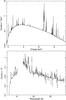Fig. 2 Simplified spectra of the Perseus cluster (top) with Hitomi and of Capella (bottom) with RGS.

We tested our method to assess the goodness of fit with two examples. In the first example, we simulated a spectrum that has approximately the shape of the Perseus cluster as measured with the Hitomi SXS instrument (Hitomi Collaboration et al. 2016). For this demonstration purpose we simplified the model by adopting an isothermal spectrum in collisional ionisation equilibrium with a temperature of 4 keV, proto-solar abundances, and an emission measure matching the flux of Perseus as measured by Hitomi. In our spectral fits, we used the temperature and emission measure of the source as free parameters. The spectrum has 5804 bins and is shown in Fig. 2, without noise, but with instrumental features included.

We scaled this spectrum in flux by factors of 10^{− k/ 2} with k ranging from 0–10, i.e. higher values of k corresponding to lower fluxes. For each flux value, we simulated 1000 spectra, performed a best fit, and determined C. We then produced a histogram of C-values and calculated the 90%, 95%, and 99% percentile points C₉₀, C₉₅, and C₉₉ of this distribution. In an actual analysis of an observed spectrum, a model would be rejected at the 90% confidence level if C>C₉₀, and this is similar for the other confidence levels. We compare these percentile points, scaled with the expected mean C_e and variance C_v, as delivered by SPEX and described in Sect. 2, in Fig. 3.

Our second example is a simulation of the spectrum of Capella with the Reflection Grating Spectrometer (RGS) of XMM-Newton. This spectrum is approximated by a single isothermal component with temperature 0.5 keV and appropriate flux for Capella. All further steps are the same as for the Perseus example. The main difference between both spectra is that while Perseus is dominated by continuum emission, owing to its high temperature, Capella is dominated by line emission, owing to its low temperature. The Capella spectrum has 1433 bins and is also shown in Fig. 2.

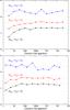Fig. 3 Percentile points 90%, 95%, and 99% for the distribution of C for simulated Perseus (top) and Capella (bottom) spectra. The expected value Ce was subtracted and the difference is scaled with $\sqrt{{\mathit{C}}_{\mathrm{v}}}$. The percentile points are shown as a function of the average number of counts in the spectra. The dotted lines show the expected percentile values if the distribution of C had been normal. These values are reached asymptotically for large numbers of counts in the spectra.

From Fig. 3 we see that for more than about 30 counts in the spectrum the percentile points C₉₀ and C₉₅ (dots connected by solid lines) are close to the values calculated from the mean value and variance of C using a Gaussian approximation (dotted lines). This holds for both examples. For C₉₅, the Gaussian approximation even works for spectra with 10 counts.

But even going down to about 5 counts does not result in dramatic differences. In general one needs to be very cautious with spectra that have so few counts. For instance, 30 counts correspond to an average number of counts per bin of 0.005 and 0.02 only for the scaled Perseus and Capella spectra, respectively.

5. Conclusion

The C-statistic can be used to estimate the goodness of fit of a model in the vast majority of all cases. When the spectrum has more than 10–30 counts, the distribution of C for the tested model is close enough to a Gaussian distribution for the highest confidence levels above 95%. This paper describes an algorithm that calculates the expected mean and variance of C that can be used to assess these confidence levels using a simple normal distribution.

Note added in proof. Equation (3), attributed here to Castor, was introduced also by Baker & Cousins (1984).

Acknowledgments

SRON is supported financially by NWO, The Netherlands Organization for Scientific Research. I thank the referee for useful comments.

References

All Figures

	Fig. 1 Expected value of the contribution per bin to C, and its rms uncertainty as a function of the mean expected number of counts μ.
In the text

	Fig. 2 Simplified spectra of the Perseus cluster (top) with Hitomi and of Capella (bottom) with RGS.
In the text

Fig. 3 Percentile points 90%, 95%, and 99% for the distribution of C for simulated Perseus (top) and Capella (bottom) spectra. The expected value Ce was subtracted and the difference is scaled with $\sqrt{{\mathit{C}}_{\mathrm{v}}}$. The percentile points are shown as a function of the average number of counts in the spectra. The dotted lines show the expected percentile values if the distribution of C had been normal. These values are reached asymptotically for large numbers of counts in the spectra.

In the text

References

- Arnaud, K. A. 1996, in Astronomical Data Analysis Software and Systems V, eds. G. H. Jacoby, & J. Barnes, ASP Conf. Ser., 101, 17 [Google Scholar]
- Baker, S., & Cousins, R. D. 1984, Nucl. Inst. Meth. Phys. Res., 221, 437 [NASA ADS] [CrossRef] [Google Scholar]
- Cash, W. 1979, ApJ, 228, 939 [NASA ADS] [CrossRef] [Google Scholar]
- Freeman, P., Doe, S., & Siemiginowska, A. 2001, in Astronomical Data Analysis, eds. J.-L. Starck, & F. D. Murtagh, Proc. SPIE, 4477, 76 [Google Scholar]
- Gehrels, N. 1986, ApJ, 303, 336 [NASA ADS] [CrossRef] [Google Scholar]
- Hitomi Collaboration, Aharonian, F., Akamatsu, H., et al. 2016, Nature, 535, 117 [Google Scholar]
- Kaastra, J. S., Mewe, R., & Nieuwenhuijzen, H. 1996, in UV and X-ray Spectroscopy of Astrophysical and Laboratory Plasmas, eds. K. Yamashita, & T. Watanabe, 411 [Google Scholar]
- Mighell, K. J. 1999, ApJ, 518, 380 [NASA ADS] [CrossRef] [Google Scholar]
- Nousek, J. A., & Shue, D. R. 1989, ApJ, 342, 1207 [NASA ADS] [CrossRef] [Google Scholar]
- Wheaton, W. A., Dunklee, A. L., Jacobsen, A. S., et al. 1995, ApJ, 438, 322 [NASA ADS] [CrossRef] [Google Scholar]