| Issue |
A&A
Volume 604, August 2017
|
|
|---|---|---|
| Article Number | A129 | |
| Number of page(s) | 19 | |
| Section | Stellar atmospheres | |
| DOI | https://doi.org/10.1051/0004-6361/201730779 | |
| Published online | 25 August 2017 | |
The formation of the Milky Way halo and its dwarf satellites; a NLTE-1D abundance analysis
I. Homogeneous set of atmospheric parameters⋆
1 Universitäts-Sternwarte München, Scheinerstr. 1, 81679 München, Germany
e-mail: This email address is being protected from spambots. You need JavaScript enabled to view it.
2 Institute of Astronomy, Russian Academy of Sciences, 119017 Moscow, Russia
e-mail: This email address is being protected from spambots. You need JavaScript enabled to view it.
3 Laboratoire d’Astrophysique, École Polytechnique Fédérale de Lausanne (EPFL), Observatoire de Sauverny, 1290 Versoix, Switzerland
4 GEPI, Observatoire de Paris, CNRS, Université Paris Diderot, 92125 Meudon Cedex, France
Received: 14 March 2017
Accepted: 19 April 2017
Abstract
We present a homogeneous set of accurate atmospheric parameters for a complete sample of very and extremely metal-poor stars in the dwarf spheroidal galaxies (dSphs) Sculptor, Ursa Minor, Sextans, Fornax, Boötes I, Ursa Major II, and Leo IV. We also deliver a Milky Way (MW) comparison sample of giant stars covering the − 4 < [Fe/H] < − 1.7 metallicity range. We show that, in the [Fe/H] ≿ − 3.7 regime, the non-local thermodynamic equilibrium (NLTE) calculations with non-spectroscopic effective temperature (Teff) and surface gravity (log g) based on the photometric methods and known distance provide consistent abundances of the Fe i and Fe ii lines. This justifies the Fe i/Fe ii ionisation equilibrium method to determine log g for the MW halo giants with unknown distance. The atmospheric parameters of the dSphs and MW stars were checked with independent methods. In the [Fe/H] > − 3.5 regime, the Ti i/Ti ii ionisation equilibrium is fulfilled in the NLTE calculations. In the log g − Teff plane, all the stars sit on the giant branch of the evolutionary tracks corresponding to [Fe/H] = − 2 to − 4, in line with their metallicities. For some of the most metal-poor stars of our sample, we achieve relatively inconsistent NLTE abundances from the two ionisation stages for both iron and titanium. We suggest that this is a consequence of the uncertainty in the Teff-colour relation at those metallicities. The results of this work provide the basis for a detailed abundance analysis presented in a companion paper.
Key words: stars: abundances / stars: atmospheres / stars: fundamental parameters / galaxies: dwarf / Local Group
Tables A.1 and A.2 are also available at the CDS via anonymous ftp to cdsarc.u-strasbg.fr (130.79.128.5) or via http://cdsarc.u-strasbg.fr/viz-bin/qcat?J/A+A/604/A129
© ESO, 2017
1. Introduction
Current knowledge of the first stages of star formation in galaxies is still poor. To complete our understanding, it is important to understand whether or not galaxies follow a universal path, independently from their final masses. In order to do this we need to elucidate several areas, including the level of homogeneity of the interstellar medium from which stars form, and how this medium evolves, and also the stellar initial mass function of the first stars.
These questions can essentially only be addressed in depth in the Local Group. Only there can we analyse individual stars in sufficient detail to guide our understanding of the physics of star formation, supernovae feeback, and the early build-up of galaxies. The comparison between ultra-faint, classical dwarf spheroidal galaxies (UFDs, dSphs), and the Milky Way population offers a fantastic opportunity to probe different galaxy masses, star formation histories, and levels of chemical enrichement. Both nucleosynthetic processes and galaxy formation models largely benefit from the diversity of the populations sampled that way.
We are, however, facing two limitations:
-
a)
Heterogeneity in the samples. Since the first high-resolutionspectroscopic study of the very metal-poor (VMP, [Fe/H]1 < − 2)stars in the Draco, Sextans, and Ursa Minor dSphs (Shetroneet al. 2001) much of theobservational efforts have been invested to obtain de-tailed chemical abundances of stars in the Milky Waysatellites. The largest samples of the VMP and extremelymetal-poor (EMP, [Fe/H] < − 3) stars, which were observedwith a spectral resolving power of R> 20 000, are available in the lit-erature for the classical dSphs in Sculptor (Tafelmeyeret al. 2010; Kirby& Cohen 2012; Jablonkaet al. 2015; Simonet al. 2015) and Ursa Minor(Sadakane et al. 2004; Cohen& Huang 2010; Kirby& Cohen 2012; Uralet al. 2015). As for the UFDs,the most studied cases are Boötes I (Feltzinget al. 2009; Norriset al. 2010; Gilmoreet al. 2013; Ishigakiet al. 2014; Frebelet al. 2016), Segue 1(Frebel et al. 2014), ComaBerenices and Ursa Major II (Frebelet al. 2010). Unfortunately, thetotal number of new stars in each individual paper never ex-ceeds seven. Therefore, it is common to combine these samplesaltogether. However, they were gathered with different spec-troscopic setups and analysed in different ways, with differentmethods of determination of atmospheric parameters, differentmodel atmospheres, radiation transfer and line formation codes,and line atomic data. Thus, studying this collection can easily leadto inaccurate conclusions.
-
b)
Heterogeneity arises also, when applying the LTE assumption for determination of the chemical abundances of the stellar samples with various effective temperatures, surface gravities, and metallicities. Individual stars in the dSphs that are accessible to high-resolution spectroscopy are all giants, and line formation, in particular in the metal-poor atmospheres, is subject to the departures from LTE because of low electron number density and low ultra-violet (UV) opacity. For each galaxy, the Milky Way or its satellites, the sampled range of metallicity can be large (Tolstoy et al. 2009). Similarly, the position of the stars along the red giant branch (i.e. their effective temperatures and surface gravities) can vary between samples.
In the literature, determinations of atmospheric parameters and chemical abundances based on the non-local thermodynamic equilibrium (NLTE) line formation were reported for Milky Way stars spanning a large interval of metallicities (Hansen et al. 2013; Ruchti et al. 2013; Bensby et al. 2014; Sitnova et al. 2015; Zhao et al. 2016), however, none has yet treated both the Milky Way and the dSph stellar samples.
In this context, our project aims at providing a homogeneous set of atmospheric parameters and elemental abundances for the VMP and EMP stars in a set of dSphs as well as for a Milky Way halo comparison sample. By employing high-resolution spectral observations and treating the NLTE line formation, our desire is to push the accuracy of the abundance analysis to the point where the trends of the stellar abundance ratios with metallicity can be robustly discussed.
In the following, we present the determination of accurate atmospheric parameters: effective temperatures, Teff, surface gravities, log g, iron abundances (metallicity, [Fe/H]), and microturbulence velocities, ξt. We rely on the photometric methods, when deriving the effective temperatures. The surface gravities are based on the known distance for the dSph stars and establishing the NLTE ionisation equilibrium between Fe i and Fe ii for the Milky Way stars. The metallicities and microturbulence velocities were determined from the NLTE calculations for Fe i-ii. A companion paper focuses on the NLTE abundances of a large set of chemical elements, spanning from Na to Ba, and the analysis of the galaxy abundance trends.
The paper is structured as follows: Sect. 2 describes the stellar sample and the observational material. Effective temperatures are determined in Sect. 3. In Sect. 4, we demonstrate that the Fe i/Fe ii ionisation equilibrium method is working in NLTE down to extremely low metallicities and we derive spectroscopic surface gravities for the Milky Way (MW) giant sample. The stellar atmosphere parameters are checked with the Ti i/Ti ii ionisation equilibrium and a set of theoretical evolutionary tracks in Sect. 5. Comparison with the literature is conducted in Sect. 6. Section 7 summarises our results.
2. Stellar sample and observational material
Our sample of VMP stars in dSphs has been selected from published datasets by requesting:
-
1.
the availability of spectra at high spectral resolution(R = λ/ Δλ ≥ 25 000); and
-
2.
good photometry, enabling the determination of the atmospheric parameters, Teff and log g, by non-spectroscopic methods.
We selected 36 stars in total in the classical dSphs Sculptor (Scl), Ursa Minor (UMi), Fornax (Fnx), and Sextans (Sex) and the ultra-faint dwarfs Boötes I, Ursa Major II (UMa II), and Leo IV (Table A.3). This sample covers the − 4 ≤ [ Fe / H ] < − 1.5 metallicity range. It is assembled from the following papers:
-
Sculptor: Jablonkaet al. (2015), Kirby& Cohen (2012), Simonet al. (2015), and Tafelmeyeret al. (2010);
-
Ursa Minor: Cohen & Huang (2010), Kirby & Cohen (2012), and Ural et al. (2015);
-
Fornax and Sextans: Tafelmeyer et al. (2010);
-
Boötes I: Gilmore et al. (2013), Norris et al. (2010), and Frebel et al. (2016, Boo-980);
-
UMa II: Frebel et al. (2010);
-
Leo IV-S1: Simon et al. (2010).
The comparison sample in the Milky Way halo was selected from the literature based on the following criteria.
-
1.
The MW and dSph stellar samples should have similartemperatures, luminosities, and metallicity range: cool giantswith Teff ≤ 5250 K and [Fe/H] < − 2.
-
2.
High spectral resolution (R> 30 000) observational material should be accessible.
-
3.
Photometry in the V, I, J, K bands must be available to derive photometric Teff.
Binaries, variables, carbon-enhanced stars, and Ca-poor stars were ignored.
As a result, the MW comparison sample includes 12 stars from Cohen et al. (2013, hereafter, CCT13), two stars from Mashonkina et al. (2010, 2014), and nine stars from Burris et al. (2000). For the latter subsample we used spectra from the VLT2/UVES2 and CFHT/ESPaDOnS3 archives.
The characteristics of the stellar spectra, which were used in this analysis, are summarised in Table A.3. Details of the observations and the data reduction can be found in the original papers. We based our study on the published equivalent widths (Wobss) and line profile fitting, where the observed spectra are available, as indicated in Table A.3.
3. Effective temperatures
This study is based on photometric effective temperatures. We could adopt the published data for about half of our sample, namely:
-
stars in the Sculptor, Fornax, and Sextans dSphs, for which Teff wasdetermined in Tafelmeyeret al. (2010) andJablonkaet al. (2015) fromthe V − I,V − J, and V − K colours and the calibration of Ramírez &Meléndez (2005b) using the CaT metallicityestimates;
-
stars in Boötes I, for which Teff was based on the B − V colour and griz photometry (Norris et al. 2010; Gilmore et al. 2013);
-
the CCT13 stellar subsample, with Teff based on V − I, V − J, and V − K colours that were matched using the predicted colour grid of Houdashelt et al. (2000); and
-
HD 122563, for which Teff is based on angular diameter measurements (Creevey et al. 2012).
For the rest of the sample, we determined the photometric effective temperatures ourselves. The J, H, K magnitudes were taken from Skrutskie et al. (2006, 2MASS All Sky Survey), unless another source is indicated. The calibration of Ramírez & Meléndez (2005b) was applied and the interstellar reddening was calculated assuming AV = 3.24EB − V. The optical photometry was gathered from a range of sources, as follows.
-
For the star 1019417 in the Sculptor dSph, the star 980 in Boötes I, and the UMa II stars, we used the Adelman-McCarthy et al. (2009)ugriz magnitudes. They were transformed into V and I magnitudes, by applying the empirical colour transformations between the SDSS and Johnson-Cousins photometry for metal-poor stars of Jordi et al. (2006). We checked these transformations on the MW star BD +44°2236, for which both the VRI and gri magnitudes are accurate within 0.0007 mag and 0.04 mag, respectively. The difference between the transformed and observed Johnson-Cousins magnitudes amounts to 0.027 mag, hence does not exceed the statistical error given by Jordi et al. (2006).
-
In the Sculptor dSph, for the stars 11_1_4296, 6_6_402, and S1020549 we used the V − I and V − K colours and metallicities from Simon et al. (2015). The metallicity of the star 1019417 was taken from Kirby & Cohen (2012). We adopted EB − V = 0.018 as in Tafelmeyer et al. (2010) and Jablonka et al. (2015).
-
In the Ursa Minor dSph, the V and I magnitudes and metallicities were taken from Cohen & Huang (2010) for the stars COS233, JI19, 28104, 33533, 36886, and 41065, from Ural et al. (2015) for the stars 396, 446 and 718, and from Kirby & Cohen (2012) for the star 20103. Employing the Schlegel et al. (1998) maps, we determined a colour excess of EB − V = 0.03.
-
For the UMa II dSph stars, metallicities were taken from Frebel et al. (2010), and EB − V = 0.10 (Schlegel et al. 1998).
-
For Boo-980, its effective temperature is based on the V − I colour only, given the large errors of the J and K magnitudes. The metallicity is taken from Frebel et al. (2016). We adopted a colour excess of EB − V = 0.02 from Schlegel et al. (1998).
-
For Leo IV-S1, the V − J and V − K colours as well as EB − V = 0.025 were adopted from de Jong et al. (2010, and priv. comm.) .
-
For the Milky Way stars HE2252-4225 and HE2327-5642 the photometry was taken from Beers et al. (2007) and the metallicities from Mashonkina et al. (2014) and Mashonkina et al. (2010), respectively. For both stars, a colour excess of EB − V = 0.013 was adopted according to Schlegel et al. (1998).
-
For the remaining eight MW halo giants we used the V magnitudes from the VizieR Online Data Catalogue4 (Ducati 2002, HD 2796, HD 4306, HD 128279), the Tycho-2 catalogue5 (Høg et al. 2000, HD 108317, BD − 11° 0145), Norris et al. (1985, HD 218857), Soubiran et al. (2010, HD 8724), and González Hernández & Bonifacio (2009, CD − 24°. The colour excess EB − V was estimated for each star from the analysis of their position on the (B − V) versus (V − J) diagram. The metallicities were taken from Burris et al. (2000). The final effective temperatures were obtained by averaging the individual ones from the V − J, V − H, and V − K colours.
Table A.4 lists the adopted effective temperatures.
4. Surface gravities
We need to apply two different methods to determine surface gravities of our stellar sample. The determination of log g of the dSph stars benefits from their common distance. Most of the Milky Way stars have no accurate distances, and we rely on the spectroscopic method that is based on the NLTE analysis of lines of iron in the two ionisation stages. Using the dSph stars with non-spectroscopic log g, we prove that the Fe i/Fe ii ionisation equilibrium method is working for VMP and EMP giants.
4.1. Photometric methods
Surface gravity of the dSph stars can be calculated by applying the standard relation between log g, Teff, the absolute bolometric magnitude Mbol, and the stellar mass M. This is the method that we rely on in this study, and we denote such a gravity log gd. We assumed M = 0.8 M⊙ for our RGB sample stars. The adopted distances are as follows.
-
Sculptor, Fornax, and Sextans: d = 85.9 kpc, 140 kpc, and 90 kpc, respectively, taken from Jablonka et al. (2015) and Tafelmeyer et al. (2010);
-
Leo IV-S1: d = 154 ± 5 kpc (Moretti et al. 2009);
-
Ursa Minor: d = 69 ± 4 kpc (Mighell & Burke 1999);
-
UMa II: d = 34.7 ± 2 kpc (Dall’Ora et al. 2012);
-
Boötes I: d = 60 ± 6 kpc (Belokurov et al. 2006).
In case of the Sculptor, Fornax, and Sextans dSphs, we used the log gd values derived by Jablonka et al. (2015) and Tafelmeyer et al. (2010), which were obtained with the bolometric correction of Alonso et al. (1999b). For the Sculptor dSph, Pietrzyński et al. (2008) derived statistical and systematic errors of the distance modulus as 0.02 mag and 0.12 mag, respectively, leading to a maximum shift of 0.05 dex in log gd. An uncertainty of 80 K in Teff results in uncertainty of 0.03 dex in log gd.
The same method was applied to most of the rest of our dSph stars. If we used the V magnitudes, then we adopted the bolometric correction from Alonso et al. (1999b). If the SDSS i magnitude was used, then the bolometric correction was from Casagrande & VandenBerg (2014). The sources of photometry were cited in the previous section.
Statistical error of the distance-based surface gravity was computed as the quadratic sum of errors of the star’s distance, effective temperature, mass, visual magnitude, and bolometric correction:  (1)Here, σlog d is taken for given dSph and σlog T for each individual star, while we adopt a common uncertainty of 0.02 M⊙ in the star’s mass, σV = 0.02 mag, and σBC = 0.02 mag.
Another method to determine the surface gravity relies on placing stars on isochrones. The gravities derived in this way are denoted log gph.
In Boötes I, log gph were determined together with Teff by Norris et al. (2010) and Gilmore et al. (2013, adopting the NY analysis) from the (g − r)0 and (r − z)0 colours, assuming that the stars were on the red giant branch and iteratively using the synthetic ugriz colours of Castelli6 and the Yale-Yonsei Isochrones (Demarque et al. 2004)7, with an age of 12 Gyr.
For most of the Boötes I stars, the absolute difference between log gd and log gph does not exceed 0.06 dex. Therefore, we adopted the original surface gravities of Gilmore et al. (2013) as final. In contrast, for Boo-94 and Boo-1137, we found log gd greater than log gph by 0.21 dex and 0.19 dex, respectively. As shown in Sect. 4.2.4, log gd leads to consistent NLTE abundances from lines of Fe i and Fe ii in Boo-94 and a smaller difference between the two ionisation stages for Boo-1137. Consequently, we adopted the log gd value as final surface gravity for these two stars.
As for the Milky Way sample, Cohen et al. (2013) applied an approach similar to that of Norris et al. (2010) and Gilmore et al. (2013) to determine photometric log gph values for their stellar sample, using the VIJK photometry.
4.2. Spectroscopic methods
4.2.1. Line selection and atomic data
Following Jablonka et al. (2015), we did not use the Fe i lines with low excitation energy of the lower level, Eexc < 1.2 eV. This is because our study is based on classical plane-parallel (1D) model atmospheres, while the low-excitation lines are predicted to be affected by hydrodynamic phenomena (3D effects) in the atmosphere to a greater degree than the higher excitation lines (Collet et al. 2007; Hayek et al. 2011; Dobrovolskas et al. 2013). For example, in the 4858/2.2/− 3 model, the abundance correction (3D-1D) amounts to − 0.8 dex and 0.0 dex for the Fe i lines arising from Eexc = 0 and 4 eV, respectively (Collet et al. 2007, W = 50 mÅ). In general, we do not see such a large discrepancy between the low- and high-excitation lines of Fe i in the investigated stars. Nevertheless, in Scl07-50, for example, the difference in LTE abundances between the Eexc< 1.2 eV and Eexc> 1.2 eV lines amounts to 0.36 dex.
The spectral lines used in the abundance analysis are listed in Table A.1 together with their atomic parameters. The gf-values and the van der Waals damping constants, Γ6, based on the perturbation theory (Barklem et al. 2000) were taken from VALD3 (Ryabchikova et al. 2015), at the exception of Fe ii, for which we used the gf-values from Raassen & Uylings (1998) that were corrected by + 0.11 dex, following the recommendation of Grevesse & Sauval (1999).
4.2.2. Codes and model ingredients
The present investigation is based on the NLTE methods developed in our earlier studies and described in detail by Mashonkina et al. (2011) for Fe i-ii and Sitnova et al. (2016) for Ti i-ii. A comprehensive model atom for iron included, for the first time, not only measured but also predicted energy levels of Fe i, about 3000, in total, and used the most up-to-date radiative data on photoionisation cross-sections and transition probabilities. A similar approach was applied to construct a model atom for titanium, with more than 3600 measured and predicted energy levels of Ti i and 1800 energy levels of Ti ii and using quantum mechanical photoionisation cross-sections. To solve the coupled radiative transfer and statistical equilibrium (SE) equations, we employed a revised version of the DETAIL code (Butler & Giddings 1985) based on the accelerated lambda iteration (ALI) method described in Rybicki & Hummer (1991, 1992). An update of the opacity package in DETAIL was presented by Mashonkina et al. (2011).
We first calculated the LTE elemental abundances with the code WIDTH98 (Kurucz 2005, modified by Vadim Tsymbal, priv. comm.). The NLTE abundances were then derived by applying the NLTE abundance corrections, ΔNLTE = log εNLTE − log εLTE. For each line and set of stellar atmospheric parameters, these corrections were obtained either by interpolation of the pre-computed correction grid of Mashonkina et al. (2016) or by direct computation with the code LINEC (Sakhibullin 1983). We verified the consistency of the two codes, WIDTH9 and LINEC, in LTE.
We used the MARCS homogeneous spherical atmosphere models with standard abundances (Gustafsson et al. 2008), as provided by the MARCS website9. They were interpolated at the necessary Teff, log g, and iron abundance [Fe/H], using the FORTRAN-based routine written by Thomas Masseron and available on the same website.
All our codes treat the radiation transfer in plane-parallel geometry, while using the model atmospheres calculated in spherically symmetric geometry. Such an approach is referred to by Heiter & Eriksson (2006) as s_p (inconsistent), in contrast to the consistent spherical (s_s) approach. Using lines of Fe i and Fe ii, Heiter & Eriksson (2006) evaluated the abundance differences between s_p and s_s for solar metallicity models, varying temperature and surface gravity. All the differences are negative, independently of whether the minority or majority species is considered and also independently of the stellar parameters. For example, for the models Teff/ log g = 4500/1.0 and 5000/1.5, the abundance difference (s_p − s_s) is smaller than 0.02 dex for the lines with an equivalent width of W< 120 mÅ. Similar calculations were performed by Ryabchikova et al. (in prep.) for VMP stars. In line with Heiter & Eriksson (2006), the resulting (s_p − s_s) differences are overall negative and, for each model atmosphere, their magnitude depends only on the line strength. For example, for the 4780/1.06/− 2.44 model, (s_p − s_s) does not exceed 0.06 dex for the W< 120 mÅ lines. Thus, the sphericity effects on the abundance differences between Fe i and Fe ii are minor. Our spectroscopic determination of stellar surface gravities is robust.
In a similarly homogeneous way, all the codes we used do treat continuum scattering correctly, such that scattering is taken into account not only in the absorption coefficient, but also in the source function.
4.2.3. Calibration of SH
We now concentrate on the main source of uncertainties in NLTE calculations for metal-poor stellar atmospheres: the treatment of the inelastic collisions with the H i atoms. This study is based on the Drawin (1968) approximation, as implemented by Steenbock & Holweger (1984), with the Drawinian rates scaled by a factor of SH. It is worth noting that the H i impact excitation is taken into account also for the forbidden transitions, following Takeda (1994) and using a simple relation between hydrogen and electron collisional rates, 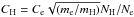 . The same SH value was applied as for the Drawinian rates. Using slightly different samples of the reference stars, Mashonkina et al. (2011), Bergemann et al. (2012), and Sitnova et al. (2015) estimated SH empirically as 0.1, 1, and 0.5, respectively.
In the present study, we chose to calibrate SH with the seven VMP Sculptor giants from Tafelmeyer et al. (2010) and Jablonka et al. (2015), for which accurate distance-based surface gravities are available. For each of these stars, the iron abundance has been derived from the Fe i and Fe ii lines under various line-formation assumptions, that is, NLTE conditions with SH = 0.1, 0.5, 1, and under the LTE hypothesis. We did not use any strong lines (Wobs> 120 mÅ) in order to minimise the impact of the uncertainties in both sphericity (see Sect. 4.2.2) and Γ6-values on our results.
The differences in the mean abundances derived from lines of Fe i, log εFeI, and Fe ii, log εFeII, are displayed in Fig. 1. At [Fe/H] > − 3.5, log εFeI is systematically lower than log εFeII under the LTE assumption, although the difference Fe I – Fe II = log εFeI − log εFeII nowhere exceeds 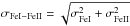 , which ranges between 0.19 dex and 0.27 dex. Here, the sample standard deviation:
 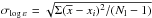 , determines the dispersion in the single line measurements around the mean for a given ionisation stage and Nl is the number of measured lines. For given chemical species, the line-to-line scatter is caused by uncertainties in the continuum normalisation, line-profile fitting (independent of whether in spectral synthesis or equivalent width measurements), and atomic data, and, thus, of random origin.
Any NLTE treatment results in weaker Fe i lines as compared to the LTE approximation. This is due to the over-ionisation driven by super-thermal radiation of non-local origin below the ionisation thresholds of the Eexc = 1.4–4.5 eV levels. It therefore induces positive NLTE abundance corrections, as shown in Fig. 2. For a given spectral line and model atmosphere, ΔNLTE increases with decreasing SH. At given SH, the NLTE effect increases with decreasing metallicity. A thorough discussion of the NLTE abundance corrections for an extended list of the Fe i lines is given by Mashonkina et al. (2011) and Mashonkina et al. (2016).
At SH = 0.5, ΔNLTE does not exceed 0.15 dex in the 4570/1.17/− 2.1 model, while it ranges between 0.15 dex and 0.45 dex for different lines in the 4670/1.13/− 3.6 model. The departures from LTE are small for Fe ii, such that ΔNLTE nowhere exceeds 0.01 dex for SH≥ 0.5 and reaches +0.02 dex for SH = 0.1 in the most iron-poor models.
 |
Fig. 1 Abundance differences between the two ionisation stages for iron, Fe I – Fe II = log εFeI – log εFeII, for the seven Sculptor dSph stars of Tafelmeyer et al. (2010) and Jablonka et al. (2015), for the LTE and NLTE line-formation scenarios. The open squares correspond to LTE and the filled rhombi, squares, and circles to NLTE from calculations with SH = 0.1, 0.5, and 1, respectively. The error bars correspond to σFeI − FeII for NLTE(SH = 0.5). |
Our test calculations disfavour SH = 0.1 because this leads to higher abundance from Fe i than from Fe ii for all stars apart from ET0381, the least metal-poor star of our sample, for which SH = 0.1 leads to exactly identical abundances between the two ionisation stages.
In the [Fe/H] > − 3.5 regime, SH = 1 leads to somewhat negative average difference between Fe i and Fe ii (− 0.06 ± 0.05 dex). Therefore there is no reason to increase SH above 0.5, which provides a very satisfactory balance between the two ionisation stages. The particular case of our most MP stars, which obviously cannot be tackled with SH, is addressed later in Sect. 5.1.1.
NLTE abundances of iron in the Sculptor dSph stars computed using accurate Fe i + H i rate coefficients and classical Drawinian rates.
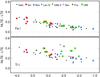 |
Fig. 2 Differences between the NLTE and LTE abundance derived from lines of Fe i (top panel) and Ti i (bottom panel) in the stars in Sculptor (red circles), Ursa Minor (green circles), Fornax (rhombi), Sextans (squares), Boötes I (triangles), UMa II (inverted triangles), and Leo IV (5-pointed star) dSphs and the MW halo stars (small black circles). |
Not only the Fe i/Fe ii ionisation, but also the Fe i excitation equilibrium was achieved, when keeping the photometric values of Teff and log gd. Figure 3 displays the NLTE (SH = 0.5) abundances,  , of the individual lines of Fe i and Fe ii in Scl002_06 and Fnx05-42 as a function of Eexc and Wobs. These abundances are put on a classical scale with log εH = 12. In most cases, NLTE leads to smaller slopes (in absolute value) than LTE in the relation (Fe i) versus Eexc, for example of − 0.03 dex/eV instead of − 0.11 dex/eV for Scl031_11.
In sharp contrast to the above description, our two most metal-poor stars with [Fe/H] < − 3.5 already have consistent Fe i- and Fe ii-based abundances in the LTE approximation, while NLTE leads to Fe I – Fe II = 0.21 ± 0.16 dex for Scl031_11 and 0.28 ± 0.24 dex for Scl07-50, even for SH = 1. At face value, the Fe ii abundance relies on only two lines, at 4923 Å and 5018 Å, with rather uncertain gf-values. Nevertheless, we note that decreasing Teff by 170 K and 200 K for Scl031_11 and Scl07-50, respectively, leads to consistent NLTE iron abundances from the two ionisation stages, when adopting SH = 0.5.
 |
Fig. 3 NLTE(SH = 0.5) abundances derived from the Fe i (open circles) and Fe ii (filled circles) lines in the selected stars as a function of Wobs (left column) and Eexc (right column). In each panel, the dotted line shows the mean iron abundance determined from the Fe i lines and the shaded grey area indicates the scatter around the mean value, as determined by the sample standard deviation. |
Barklem (2016) has treated a theoretical method for the estimation of cross-sections and rates for excitation and charge-transfer processes in low-energy hydrogen-atom collisions with neutral atoms, based on an asymptotic two-electron model of ionic-covalent interactions in the neutral atom-hydrogen-atom system and the multichannel Landau-Zener model. The rate coefficients computed for Fe i+H i collisions were applied by Amarsi et al. (2016), Nordlander et al. (2017), and Lind et al. (2017) to the NLTE analyses of lines of iron in the reference metal-poor stars. Paul Barklem has kindly provided us with the Fe i+H i rate coefficients, and we applied these data to determine the iron NLTE abundances of the six stars in the Sculptor dSph. Following Amarsi et al. (2016), inelastic collisions of Fe ii with H i were treated using the scaled Drawinian rates. We adopt SH = 0.5. The obtained results are presented in Table 1. For Fe i, the NLTE – LTE abundance difference ranges between 0.13 dex and 0.38 dex, depending on the star’s metallicity. In the four stars, NLTE leads to acceptable abundance difference of no more than 0.10 dex between Fe i and Fe ii. However, implementing the most up-to-date Fe i + H i collision data in our NLTE model does not help to achieve the Fe i/Fe ii ionisation equilibrium for the [Fe/H] ≃ − 3.7 star.
4.2.4. Determination of log g from analysis of Fe i/Fe ii
Having realised that the Drawin (1968) approximation does not contain the relevant physics (see, for example, a critical analysis of Barklem et al. 2011) and, for different transitions in Fe i, the Drawinian rate has a different relation to a true Fe i+H i collision rate, we consider the NLTE calculations with the scaled Drawinian rates in the 1D model atmospheres as a 1D-NLTE (SH = 0.5) model that fits observations of the Fe i and Fe ii lines in our reference stars, namely, the Sculptor dSph stars with [Fe/H] > − 3.7. This model was tested further with our stellar samples in the Ursa Minor, Fornax, Sextans, Boötes I, Leo IV, and UMa II dSphs. The Fe i/Fe ii ionisation equilibrium was checked in each star, while keeping its atmospheric parameters, Teff, log gd or log gph, fixed. From there we determined the final iron abundances and the microturbulence velocites, ξt; these are presented in Table A.4. For example, we show in Fig. 3 the NLTE abundances from lines of Fe i and Fe ii in Boo-33 as functions of Wobs and Eexc, which support the derived ξt = 2.3 km s-1 and Teff = 4730 K. It is worth noting that we did not find any significant change in the slopes of the (Fe i)–log(Wλ/λ) plots between the LTE and NLTE calculations.
Error budget for log gsp of HD 8724 and HE1356-0622.
Table A.2 lists the mean NLTE abundances from each ionisation stage, Fe i and Fe ii, together with their  and number of lines measured. Systematic errors of log εFeI and log εFeII for a given star are due to the uncertainty in adopted atmospheric parameters. Our calculations show that a change of +100 K in Teff produces 0.10-0.12 dex higher abundances from lines of Fe i and has a minor effect (<0.02 dex) on the abundances from lines of Fe ii. In contrast, a change of 0.1 dex in log g has a minor effect (<0.01 dex) on Fe i and shifts log εFeII by +0.04 dex. A change of +0.2 km s-1 in ξt produces lower iron abundances by 0.02 to 0.05 dex, depending on the sample of the iron lines measured in a given star.
The LTE and NLTE (SH = 0.5) abundance differences between Fe i and Fe ii are shown in the upper panel of Fig. 4. In addition to Scl07-50 and Scl031_11, two other stars, Scl 6_6_402 ([Fe/H] = − 3.66) and Boo-1137 ([Fe/H] = − 3.76), have differences of more than 0.2 dex in the NLTE abundances between the two ionisation stages. Other than these, the average log εFeI − log εFeII difference amounts in NLTE to − 0.02 ± 0.07. It is worth noting that we have the two [Fe/H] ≃ − 3.7 stars, Scl11_1_4296 and S1020549, for which the Fe i/Fe ii ionisation equilibrium is fulfilled in NLTE. Hence, our 1D-NLTE(SH = 0.5) model can reliably be used to determine the spectroscopic gravity of stars with [Fe/H] ≿ − 3.7. Consequently, we adopted, as a final value, the spectroscopic log gsp = 1.8 instead of log gd = 1.63 for Boo-980 (4760/1.8/− 3.01).
Based on the NLTE analysis of the Fe i and Fe ii lines, we checked Teff/log g determined by Cohen et al. (2013) for their MW stellar subsample. The surface gravities were revised by +0.1 dex to +0.2 dex, well within 1σ uncertainties. The obtained microturbulence velocities are similar to those of Cohen et al. (2013) except for the four stars, for which our values are 0.2 km s-1 to 0.5 km s-1 lower. One of these stars is HE2249-1704 (4590/1.2/− 2.94), and Fig. 3 supports the derived ξt = 2 km s-1. It is worth noting that we did not include the Fe ii 3255 Å, 3277 Å, and 3281 Å lines in the analysis of BS16550-087 because they give 0.81, 0.27, and 0.44 dex higher abundances than the mean of the other twelve Fe ii lines.
For the rest of the MW stellar sample, their log g, iron abundance, and microturbulence velocity were determined in this study from the requirements that (i) the NLTE abundances from Fe i and Fe ii must be equal and (ii) lines of Fe i with different equivalent widths must yield equal NLTE abundances.
Our calculations show that a change of 0.1 dex in log εFeI – log εFeII leads to a shift of 0.23 dex and 0.19 dex in log g for the model atmospheres 4945/2.00/− 3.45 and 4560/1.29/− 1.76, respectively. Table 2 shows estimates of the random and systematic errors, σlog g(Sp) and Δlog g(Sp), of the derived spectroscopic surface gravity for the two stars, HE1356-0622 and HD 8724, which represent the most and the least metal-poor samples. The random error is contributed from the line-to-line scatter for Fe i and Fe ii that is represented by σFeI and σFeII and the uncertainty in Teff. The quadratic addition of the individual uncertainties results in σlog g(Sp) = 0.24 and 0.32 for HD 8724 and HE1356-0622, respectively.
Uncertainty in the NLTE model was assumed to be mostly produced by applying the scaled (SH = 0.5) Drawinian rates instead of quantum-mechanical rate coefficients of Barklem (2016). In all cases, this leads to less positive NLTE abundance corrections for Fe i and, thus, to systematically underestimated surface gravity. For our sample of the MW giants, Δlog g(Sp) ranges between − 0.1 dex and − 0.23 dex.
The final atmospheric parameters are presented in Table A.4. The iron abundance is defined from lines of Fe ii. For the computation of the abundances relative to the solar scale we employed log εFe, ⊙ = 7.50 (Grevesse & Sauval 1998).
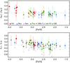 |
Fig. 4 Abundance differences between the two ionisation stages of iron, Fe I – Fe II (top panel), and titanium, Ti I – Ti II (bottom panel), in the investigated stars in Sculptor, Ursa Minor, Fornax, Sextans, Boötes I, UMa II, and Leo IV dSphs. For the MW halo stars only Ti I – Ti II is shown. Symbols as in Fig. 2. The open and filled symbols correspond to the LTE and NLTE line-formation scenario, respectively. Here, SH = 0.5 for Fe i-ii and SH = 1 for Ti i-ii. |
5. Checking atmospheric parameters with independent methods
5.1. Ti I/Ti II ionisation equilibrium
The fact that for most of our stars, titanium is accessible in the two ionisation stages, Ti i and Ti ii, opens another opportunity to check the stellar surface gravities.
We used accurate and homogeneous gf-values of the Ti i and Ti ii lines from laboratory measurements of Lawler et al. (2013) and Wood et al. (2013). The LTE and NLTE abundance differences between Ti i and Ti ii are displayed in Fig. 4.
In LTE, lines of Ti i systematically give lower abundances than the Ti ii lines by up to 0.51 dex. The only exception is S1020549, with two weak (Wobs ≃ 25 mÅ) lines of Ti i measured in its R ≃ 33 000 spectrum.
Similarly to Fe i, the main NLTE mechanism for Ti i is the UV over-ionisation, resulting in weakened lines and positive NLTE abundance corrections (Fig. 2). Since there is no accurate data on inelastic collisions of the titanium atoms with H i, we rely on the Drawinian rates (i.e. SH = 1), as recommended by Sitnova et al. (2016). For a given stellar atmosphere model, the NLTE corrections of the individual Ti i lines are of very similar orders of magnitude. For example, ΔNLTE ranges between 0.17 dex and 0.21 dex in the 5180/2.70/− 2.60 model. The departures from LTE grow towards lower metallicity, as shown in Fig. 2.
The NLTE corrections for the Ti ii lines are much smaller than those obtained for Ti i and mostly positive. They are close to 0 at [Fe/H] > − 2.5, but increase with decreasing metallicity and are close to ΔNLTE = 0.1 dex at [Fe/H] = − 4.
At [Fe/H] > − 3.5, NLTE leads to consistent abundances between Ti i and Ti ii in most of the stars, at the exception of ET0381, for which log εTiI − log εTiII = − 0.32 dex. This means that larger NLTE correction is needed for Ti i, that is, SH< 0.1, to achieve the Ti i/Ti ii ionisation equilibrium.
In contrast, the LTE assumption is working well for the [Fe/H] < − 3.5 stars, while NLTE worsens the results. This is similar to what we had found for Fe i/Fe ii. Again a decrease of Teff by 170 K for Scl031_11 partly removes a discrepancy between Ti i and Ti ii, however the remaining difference of 0.20 dex is still large.
5.1.1. The specific case of the [Fe/H] < –3.5 stars
The above analysis reflects that the four EMP stars in the dSphs do not have a satisfactory ionisation balance between Fe i and Fe ii and between Ti i and Ti ii, under the same conditions as the other stars. Here we could be facing several problems: an insufficient NLTE line-formation model and lack of thermalising processes, the lack of a proper 3D treatment of the stellar atmospheres, and/or uncertainties in determinations of the effective temperature for these EMP stars.
As shown in Sect. 4.2.3, implementing the most up-to-date Fe i + H i collision data in our NLTE model does not help to remove the abundance discrepancy between Fe i and Fe ii. Accurate calculations of the Ti i + H i collisions would be highly desirable.
Next is the 3D effects. For Fe i, we ignored the lines with Eexc < 1.2 eV. This may partly explain why we obtained a smaller difference between Fe i and Fe ii than between Ti i and Ti ii. Still, the difference between log εFeI and log εFeII ranges in NLTE (assuming SH = 0.5) between 0.30 dex and 0.36 dex for our four [Fe/H] ≾ − 3.7 stars. This is not negligible and likely cannot be removed by the 3D-NLTE calculations. Indeed, recent papers of Nordlander et al. (2017) and Amarsi et al. (2016) show that the 3D effects for Fe i are of different sign in NLTE than in LTE: 3D-1D = +0.20 dex in NLTE and − 0.34 dex in LTE in the 5150/2.2/− 5 model (Nordlander et al. 2017) and 3D-1D = +0.11 dex in NLTE and − 0.11 dex in LTE in the 6430/4.2/− 3 model (Amarsi et al. 2016). In the latter model, abundance from lines of Fe ii is higher in 3D-NLTE than 1D-NLTE. As a result, log εFeI − log εFeII is 0.05 dex smaller in 3D-NLTE than 1D-NLTE. No data is provided on Fe ii in the 5150/2.2/− 5 model. It would be important to perform the 3D-NLTE calculations for Fe i-ii in the [Fe/H] = − 4 model.
For the titanium lines in the red giant atmospheres, the 3D effects were predicted under the LTE assumption by Dobrovolskas et al. (2013). For Ti i, the (3D-1D) abundance corrections are negative, with a magnitude depending strongly on Eexc. For example, in the 5000/2.5/− 3 model, (3D-1D)= − 0.45 dex and − 0.10 dex for the Eexc = 0 and 2 eV lines at λ = 4000 Å. The 3D effects are predicted to be minor for Ti ii, with either positive or negative (3D-1D) correction of less than 0.07 dex in absolute value. Since our abundance analysis of the EMP stars is based on the low-excitation (Eexc≤ 0.85 eV) lines of Ti i, a 3D treatment (if NLTE follows LTE, see below) might help to reconcile log εTiI and log εTiII.
At this stage, we conclude that, most likely, the problem we see in NLTE with the Fe i/Fe ii and Ti i/Ti ii ionisation equilibrium in our most MP stars is related to the Teff determination, given the fact that the colour calibrations we used are in fact valid in the metallicity range − 3.5 ≤ [Fe/H]≤ 0.4 (Ramírez & Meléndez 2005b).
5.2. Spectroscopic versus Gaia DR1 gravities
As a sanity check, we computed the distance-based log g for the five stars with available Gaia parallax measurements (Gaia Collaboration 2016, Gaia Data Release 1) and available in the VizieR Online Data Catalogue. As can be seen in Table 3, for three stars, our log gsp are consistent with log gGaia within the error bars. This holds despite the fact that two of these stars, HD 4306 and BD − 11°0145, are identified as binaries.
There is one exception to this general agreement, HD 8724. It is hard to understand the source of an extremely large difference of 0.76 dex(!) between log gGaia and log gsp, in view of their small statistical and systematic errors, that is, σlog g(Gaia) = 0.08 dex, σlog g(sp) = 0.24 dex and Δlog g(sp) = − 0.1 dex. The effective temperature of HD 8724 should be increased by ~400 K in order to reconcile the Fe i and Fe ii abundances with log gGaia = 2.05. This seems very unlikely. All estimates, based on the infrared flux method (IRFM) are close to Teff = 4560 K derived in this study: Teff = 4535 K (Alonso et al. 1999a), 4540 K (Ramírez & Meléndez 2005a), and 4630 K (González Hernández & Bonifacio 2009).
Comparison of the derived spectroscopic surface gravities with that based on the Gaia parallaxes.
5.3. Checking atmospheric parameters with evolutionary tracks
We now check the effective temperatures and surface gravities that we derived by looking at the positions of the stars in the log g − Teff diagram. For this we consider the theoretical α-enhanced ([α/Fe] = 0.6) evolutionary tracks of Yi et al. (2004). Consistently with our calculation, we assumed the stellar masses to be 0.8 M⊙. Figure 5 shows that all stars correctly sit on the giant branch between the evolutionary tracks of [Fe/H] = − 2 and − 4, in line with their metallicities.
VMP stars in the MW halo and dSphs do not exactly span the same log g, Teff range. This comes as a consequence of the observational constraints. The dSphs are obviously more distant, and their stars are fainter, hence one tends to target the tip of the RGB. Since NLTE corrections depend on the stellar atmosphere parameters, in a way that, itself, depends on the species, any valuable comparison between different galaxies should be done via NLTE homogeneous analysis.
For each of five MW stars with available Gaia parallaxes, Fig. 5 indicates the two positions corresponding to log gsp and log gGaia. With log gGaia = 2.05, HD 8724 lies far from the [Fe/H] = − 2 evolutionary track. Obviously, the parallax of HD 8724 needs to be revised.
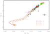 |
Fig. 5 Investigated stars compared with the evolutionary tracks of M = 0.8 M⊙ and [Fe/H] = − 2 (dash-dotted curve), − 3 (dashed curve), and − 4 (dotted curve). The crosses on the [Fe/H] = − 2 and [Fe/H] = − 4 evolutionary tracks mark stellar age of 13.4 Gyr. Symbols as in Fig. 2. For the five MW stars with the Gaia parallax available, the vertical lines connect the star’s positions corresponding to log gsp (small black circles) and log gGaia (small black circles inside larger size circles). The cross in the right part indicates log g and Teff error bars of 0.2 dex and 100 K, respectively. |
5.4. Approximate formula for microturbulence value
The relation between the microturbulence velocities and the basic atmospheric parameters Teff, log g, and [Fe/H] is not particularly well established. We take the opportunity of this study to derive an empirical formula, which we hope will be useful: ![Mathematical equation: \begin{equation} \xi_{\rm t} = 0.14 {-} 0.08 \times {\rm [Fe/H]} + 4.90 \times (\Teff/10^4) - 0.47 \times {\rm log}~g. \label{formula1} \end{equation}](/articles/aa/full_html/2017/08/aa30779-17/aa30779-17-eq173.png) (2)Figure 6 indicates the deviation from the analytical fit of the individual determinations. The largest discrepancy of 0.56 km s-1 is found for UMi-446, which also has the largest scatter of the Fe i -based abundances, with σFeI = 0.27 dex.
(2)Figure 6 indicates the deviation from the analytical fit of the individual determinations. The largest discrepancy of 0.56 km s-1 is found for UMi-446, which also has the largest scatter of the Fe i -based abundances, with σFeI = 0.27 dex.
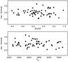 |
Fig. 6 Differences between the microturbulence velocity determined in this study for individual stars and that calculated with formula (2) as a function of metallicity (top panel) and effective temperature (bottom panel). |
We tested the validity of Eq. (2) on two ultra metal-poor (UMP) stars, HE 0107-5240 (5100/2.2/− 5.3) and HE 0557-4840 (4900/2.2/− 4.8). Our analytical fit gives ξt = 2.0 km s-1 and 1.9 km s-1, very close to the determinations of Christlieb et al. (2004, 2.2 km s-1 and Norris et al. (2007, 1.8 km s-1, respectively. Hence, we can only recommend using Eq. (2) to calculate microturbulence velocities of EMP and UMP giants.
6. Comparison with other studies
The references to the different works from which our sample was built are listed in Sect. 2. While we produced a homogeneous set of atmospheric parameters for the dSphs and MW populations that has no counterpart, it is interesting to look back and identify the origin of the changes. Not all parameters have been impacted in the same way. For each star, Fig. 7 compares Teff, ξt, log g, and [Fe/H] in this study and their previously published values.
The parameters of the Milky Way sample have hardly been modified at the exception of one or two stars. In contrast, the dSph sample has been notably impacted by the revision of the stellar atmospheric parameters and the NLTE treatment. These changes clearly depend on the original technique of analysis.
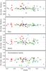 |
Fig. 7 Differences in atmospheric parameters, namely, Teff, log g, [Fe/H], and ξt (in km s-1), of the investigated stars between this and other studies. See text for references. Symbols as in Fig. 2. |
6.1. log g
The surface gravity is the atmospheric parameter that has changed the least.
We find that, for the dSphs, our final log g values agree with the published ones. This is likely a consequence of the fact that some studies used the distance-based log g as an initial estimate of the stellar surface gravity, which was then revised spectroscopically (Cohen & Huang 2010; Jablonka et al. 2015; Kirby & Cohen 2012; Tafelmeyer et al. 2010). Others, such as Gilmore et al. (2013), Norris et al. (2010), determined log g from the isochrone method. Both methods are close to our methodology.
There is one exception to this general agreement though. Surprisingly large discrepancies of 0.65 dex and 1.23 dex between the distance-based (this study) and the LTE spectroscopic surface gravities (Frebel et al. 2010) were found for UMa II-S1 and UMa II-S2. They are much larger than the errors of log gd, 0.07 dex and 0.05 dex, respectively (Table A.4), and cannot arise only due to the LTE assumption because, at given atmospheric parameters, the NLTE abundance corrections for lines of Fe i are of the order of 0.07–0.08 dex, which are propagated to no more than 0.2 dex for an error of the log gsp.
For the MW giant sample, the literature data on log g were mostly obtained from non-spectroscopic methods, that is, either the star’s absolute magnitude and/or its implied position in the colour-magnitude diagram and/or an average Teff versus log g relationship for MP giants. The differences between these data and our NLTE spectroscopic determinations mostly do not exceed 0.2 dex in absolute value.
6.2. Teff
We have mentioned that this study is partly based on published photometric temperatures. This is the case of the Boötes I stars (Norris et al. 2010; Gilmore et al. 2013) and Cohen et al. (2013) sample of MW stars. For most of the rest of the sample, the difference between the published Teff and ours does not exceed 100 K. The previously published temperatures obtained by a spectroscopic method are systematically lower compared with our photometric temperatures. Such an effect has already been pointed out in the literature (see, for example Frebel et al. 2013).
6.3. Metallicity
The differences between the published [Fe/H] values and those of the present study are large. These differences could be caused by a number of combined effects, namely,
-
(i)
different treatment of line formation, that is, NLTE in this studyand LTE in all other papers and using lines of Fe ito derive final iron abundance in most cited papers that led tounderestimated [Fe/H]; in contrast, our data are consistent within0.15 dex with the values published by Cohenet al. (2013) who employed lines ofFe ii, as we do;
-
(ii)
differences in derived microturbulence velocity, and
-
(iii)
differences in the used atomic parameters, in particular, van der Waals damping constants.
In part, a change in the stellar final metallicity is related to a correction of the original parameters. For example, Leo IV-S1’s final [Fe/H] value is 0.6 dex higher than in Simon et al. (2010), as a consequence of our higher effective temperature (by 200 K from the original estimate). The Sculptor stars at [Fe/H] ~ − 3 have seen their effective temperatures substantially revised. An upward shift of about 0.2 dex in [Fe/H] is also caused by using lines of Fe ii in this study, but not Fe i under the LTE assumption, as in the literature. In the case of Sex 11-04, which sees essentially no change in Teff/log g, the Fe i-based LTE abundance of Tafelmeyer et al. (2010) is 0.34 dex lower than our determination from lines of Fe ii.
For Boo-041 we obtained an iron abundance 0.42 dex higher than that of Gilmore et al. (2013), despite similar Teff/log g = 4750 K/1.6. This cannot be due to accounting for the NLTE effects, because (NLTE – LTE)= 0.06 dex for Fe i. A difference of 0.25 dex in log εFeI appears already in LTE, and this is due to a 0.8 km s-1 lower microturbulence velocity in our study. Going back to the LTE calculations and adopting the atmospheric parameters 4750/1.6/− 1.96 and ξt = 2.8 km s-1 of Gilmore et al. (2013) results in a steep negative slope of − 0.41 for the log εFeI − log Wobs/λ plot, using 35 lines of Fe i with Eexc > 1.2 eV and Wobs< 180 mÅ. In addition, the abundance difference log εFeI − log εFeII = − 0.22 is uncomfortably large. We derived ξt = 2.0 km s-1 by minimising the trend of the NLTE abundances of the Fe i lines with Wobs. This also makes the NLTE abundances from the two ionisation stages of iron consistent within 0.11 dex.
6.4. Microturbulence
We find that the microturbulence velocities derived in this study agree well with the corresponding values of Cohen et al. (2013), but they are lower, by up to 1.2 km s-1, compared with the data from most other papers. This explains the mostly positive differences in [Fe/H] between ours and other studies. In the case of the Boötes I stars, a source of the discrepancy in ξt was fixed in a private communication with David Yong. It appears to be connected with applying outdated van der Waals damping constants in analyses of Gilmore et al. (2013).
We found a metallicity-dependent discrepancy in ξt between Cohen & Huang (2010) and this study, from +0.3 km s-1 at [Fe/H] ≃ − 2 up to +1.0 km s-1 at [Fe/H] ≃ − 3. An overestimation of microturbulence velocity by Cohen & Huang (2010) was, most probably, caused by treating Rayleigh scattering as LTE absorption.
7. Conclusions and recommendations
This paper presents a homogeneous set of accurate atmospheric parameters for a complete sample of 36 VMP and EMP stars in the classical dSphs in Sculptor, Ursa Minor, Sextans, and Fornax and the UFDs Boötes I, UMa II, and Leo IV. For the purpose of comparison between the Milky Way halo and satellite populations in a companion paper, which presents the NLTE abundances of nine chemical elements, from Na to Ba, we also derived atmospheric parameters of 23 VMP and EMP cool giants in the MW.
-
Using the dSph stars with non-spectroscopic Teff/log gparameters, we showed that the two ionisation stages,Fe i and Fe ii, have con-sistent NLTE abundances, when the inelastic collisions withH i are treated with a scaling factor of SH[en-tity!#x2009!]= 0.5 to the classic Drawinian rates. This justifiesthe Fe i/Fe ii ionisationequilibrium method used to determine surface gravity forVMP giants with unknown distances. The statistical error oflog gsp is estimated to be 0.2–0.3 dex,if the Fe i – Fe ii abundance differenceis determined with an accuracy of 0.1 dexor better. The systematic error due to the uncertainty in our1D-NLTE(SH = 0.5) model is estimated to be− 0.1 dex to − 0.23 dex depending on stellar at-mosphere parameters. We caution against applying this methodto the [Fe/H] ≾ − 3.7 stars. For our four most metal-poor stars, 1D-NLTEfails to achieve the Fe i/Fe iiionisation equilibrium.
-
For each star, the final atmospheric parameters were checked with the Ti i/Ti ii ionisation equilibrium. No imbalance was found except for the four most metal-poor stars at [Fe/H] ≤ − 3.5. We suspect that this problem is linked to uncertainty in the determination of Teff at these very low metallicities.
-
As a sanity check, we computed the distance-based log g for the five stars with available Gaia parallax measurements (Gaia Data Release 1). For three of them, log gsp is consistent within the error bars with log gGaia. However, there is one exception to this general agreement, HD 8724, with log gsp – log gGaia = − 0.76. An inspection of the star’s position in the log g − Teff plane also does not support its log gGaia = 2.05. Evidentally, the measured parallax of HD 8724 needs to be double checked.
-
The accuracy of the derived atmospheric parameters allowed us to derive an analytical relation to calculate ξt from Teff, log g, and [Fe/H].
Lessons learnt during the process of this work lead us to outline a few recommendations to accurately determine the atmospheric parameters of VMP and EMP giants:
-
Derive the effective temperature from photometric methods.
-
Attain the surface gravities from the star distances, wherever available. If not, the NLTE Fe i/Fe ii ionisation equilibrium has proven to be a robust alternative at [Fe/H] ≿ − 3.7. We caution that, at low metallicity, LTE leads to underestimation of log g by up to 0.3 dex.
-
Calculate the metallicity from the Fe ii lines, because they are only weakly sensitive to Teff variation and nearly free of the NLTE effects. Our study shows that the Fe i lines under the LTE assumption lead to underestimation of the stellar metallicity by up to 0.3 dex.
-
Check Teff and log g with theoretical evolutionary tracks.
In the classical notation, where [X/H] = log (NX/NH)star − log (NX/NH)Sun.
Acknowledgments
This study is based on observations made with ESO Telescopes at the La Silla Paranal Observatory under programme IDs 68.D-0546(A), 71.B-0529(A), 076.D-0546(A), 079.B-0672A, 081.B-0620A, 087.D-0928A, 091.D-0912A,281.B-50220A, P82.182.B-0372, and P383.B-0038 and with the Canada-France-Hawaii Telescope under programme IDs 12BS04 and 05AC23. This research used the services of the ESO Science Archive Facility and the facilities of the Canadian Astronomy Data Centre operated by the National Research Council of Canada with the support of the Canadian Space Agency. We thank Judith G. Cohen, Rana Ezzeddine, Anna Frebel, and Joshua D. Simon for providing stellar spectra, Jelte de Jong for photometric data for Leo IV-S1, and Paul Barklem for the Fe i+H i collision rate coefficients. L.M., Y.P., and T.S. are supported by the Presidium RAS Programme P-7. P.J and P.N acknowledge financial support from the Swiss National Science Foundation. T.S. acknowledges financial support from the Russian Foundation for Basic Research (grant 16-32-00695). The authors are indebted to the International Space Science Institute (ISSI), Bern, Switzerland, for supporting and funding the international teams “First stars in dwarf spheroidal galaxies” and “The Formation and Evolution of the Galactic Halo”. We made use the MARCS, SIMBAD, and VALD databases.
References
- Adelman-McCarthy, J. K., et al. 2009, VizieR Online Data Catalog: II/294 [Google Scholar]
- Alonso, A., Arribas, S., & Martínez-Roger, C. 1999a, A&AS, 139, 335 [NASA ADS] [CrossRef] [EDP Sciences] [Google Scholar]
- Alonso, A., Arribas, S., & Martínez-Roger, C. 1999b, A&AS, 140, 261 [NASA ADS] [CrossRef] [EDP Sciences] [Google Scholar]
- Amarsi, A. M., Lind, K., Asplund, M., Barklem, P. S., & Collet, R. 2016, MNRAS, 463, 1518 [NASA ADS] [CrossRef] [Google Scholar]
- Bagnulo, S., Jehin, E., Ledoux, C., et al. 2003, The Messenger, 114, 10 [NASA ADS] [Google Scholar]
- Barklem, P. S. 2016, Phys. Rev. A, 93, 042705 [NASA ADS] [CrossRef] [Google Scholar]
- Barklem, P. S., Piskunov, N., & O’Mara, B. J. 2000, A&AS, 142, 467 [NASA ADS] [CrossRef] [EDP Sciences] [MathSciNet] [PubMed] [Google Scholar]
- Barklem, P. S., Belyaev, A. K., Guitou, M., et al. 2011, A&A, 530, A94 [NASA ADS] [CrossRef] [EDP Sciences] [Google Scholar]
- Beers, T., Flynn, C., Rossi, S., et al. 2007, ApJS, 168, 128 [NASA ADS] [CrossRef] [Google Scholar]
- Belokurov, V., Zucker, D. B., Evans, N. W., et al. 2006, ApJ, 647, L111 [NASA ADS] [CrossRef] [Google Scholar]
- Bensby, T., Feltzing, S., & Oey, M. S. 2014, A&A, 562, A71 [NASA ADS] [CrossRef] [EDP Sciences] [Google Scholar]
- Bergemann, M., Lind, K., Collet, R., Magic, Z., & Asplund, M. 2012, MNRAS, 427, 27 [NASA ADS] [CrossRef] [Google Scholar]
- Burris, D. L., Pilachowski, C. A., Armandroff, T. E., et al. 2000, ApJ, 544, 302 [NASA ADS] [CrossRef] [Google Scholar]
- Butler, K., & Giddings, J. 1985, Newsletter on the analysis of astronomical spectra, 9 (University of London) [Google Scholar]
- Casagrande, L., & VandenBerg, D. A. 2014, MNRAS, 444, 392 [NASA ADS] [CrossRef] [MathSciNet] [Google Scholar]
- Christlieb, N., Gustafsson, B., Korn, A., et al. 2004, ApJ, 603, 708 [NASA ADS] [CrossRef] [Google Scholar]
- Cohen, J. G., & Huang, W. 2010, ApJ, 719, 931 [NASA ADS] [CrossRef] [Google Scholar]
- Cohen, J. G., Christlieb, N., Thompson, I., et al. 2013, ApJ, 778, 56 [NASA ADS] [CrossRef] [Google Scholar]
- Collet, R., Asplund, M., & Trampedach, R. 2007, A&A, 469, 687 [NASA ADS] [CrossRef] [EDP Sciences] [Google Scholar]
- Creevey, O. L., Thévenin, F., Boyajian, T. S., et al. 2012, A&A, 545, A17 [NASA ADS] [CrossRef] [EDP Sciences] [Google Scholar]
- Dall’ Ora, M., Kinemuchi, K., Ripepi, V., et al. 2012, ApJ, 752, 42 [NASA ADS] [CrossRef] [Google Scholar]
- de Jong, J. T. A., Martin, N. F., Rix, H.-W., et al. 2010, ApJ, 710, 1664 [NASA ADS] [CrossRef] [Google Scholar]
- Demarque, P., Woo, J.-H., Kim, Y.-C., & Yi, S. K. 2004, ApJS, 155, 667 [NASA ADS] [CrossRef] [Google Scholar]
- Dobrovolskas, V., Kučinskas, A., Steffen, M., et al. 2013, A&A, 559, A102 [NASA ADS] [CrossRef] [EDP Sciences] [Google Scholar]
- Drawin, H.-W. 1968, Z. Phys., 211, 404 [NASA ADS] [CrossRef] [EDP Sciences] [Google Scholar]
- Ducati, J. R. 2002, VizieR Online Data Catalog: II/237 [Google Scholar]
- Feltzing, S., Eriksson, K., Kleyna, J., & Wilkinson, M. I. 2009, A&A, 508, L1 [NASA ADS] [CrossRef] [EDP Sciences] [Google Scholar]
- Frebel, A., Simon, J. D., Geha, M., & Willman, B. 2010, ApJ, 708, 560 [NASA ADS] [CrossRef] [Google Scholar]
- Frebel, A., Casey, A. R., Jacobson, H. R., & Yu, Q. 2013, ApJ, 769, 57 [NASA ADS] [CrossRef] [Google Scholar]
- Frebel, A., Simon, J. D., & Kirby, E. N. 2014, ApJ, 786, 74 [NASA ADS] [CrossRef] [Google Scholar]
- Frebel, A., Norris, J. E., Gilmore, G., & Wyse, R. F. G. 2016, ApJ, 826, 110 [NASA ADS] [CrossRef] [Google Scholar]
- Gaia Collaboration (Brown, A. G. A., et al.) 2016, A&A, 595, A2 [NASA ADS] [CrossRef] [EDP Sciences] [Google Scholar]
- Gilmore, G., Norris, J. E., Monaco, L., et al. 2013, ApJ, 763, 61 [NASA ADS] [CrossRef] [Google Scholar]
- González Hernández, J. I., & Bonifacio, P. 2009, A&A, 497, 497 [NASA ADS] [CrossRef] [EDP Sciences] [Google Scholar]
- Grevesse, N., & Sauval, A. J. 1998, Space Sci. Rev., 85, 161 [NASA ADS] [CrossRef] [Google Scholar]
- Grevesse, N., & Sauval, A. J. 1999, A&A, 347, 348 [NASA ADS] [Google Scholar]
- Gustafsson, B., Edvardsson, B., Eriksson, K., et al. 2008, A&A, 486, 951 [NASA ADS] [CrossRef] [EDP Sciences] [Google Scholar]
- Hansen, C. J., Bergemann, M., Cescutti, G., et al. 2013, A&A, 551, A57 [NASA ADS] [CrossRef] [EDP Sciences] [Google Scholar]
- Hayek, W., Asplund, M., Collet, R., & Nordlund, Å. 2011, A&A, 529, A158 [NASA ADS] [CrossRef] [EDP Sciences] [Google Scholar]
- Heiter, U., & Eriksson, K. 2006, A&A, 452, 1039 [NASA ADS] [CrossRef] [EDP Sciences] [Google Scholar]
- Høg, E., Fabricius, C., Makarov, V. V., et al. 2000, A&A, 355, L27 [NASA ADS] [Google Scholar]
- Houdashelt, M. L., Bell, R. A., & Sweigart, A. V. 2000, AJ, 119, 1448 [Google Scholar]
- Ishigaki, M. N., Aoki, W., Arimoto, N., & Okamoto, S. 2014, A&A, 562, A146 [NASA ADS] [CrossRef] [EDP Sciences] [Google Scholar]
- Jablonka, P., North, P., Mashonkina, L., et al. 2015, A&A, 583, A67 [NASA ADS] [CrossRef] [EDP Sciences] [Google Scholar]
- Jordi, K., Grebel, E. K., & Ammon, K. 2006, A&A, 460, 339 [NASA ADS] [CrossRef] [EDP Sciences] [Google Scholar]
- Kirby, E. N., & Cohen, J. G. 2012, AJ, 144, 168 [NASA ADS] [CrossRef] [Google Scholar]
- Kurucz, R. L. 2005, Mem. Soc. Astron. Ital. Suppl., 8, 14 [Google Scholar]
- Lawler, J. E., Guzman, A., Wood, M. P., Sneden, C., & Cowan, J. J. 2013, ApJS, 205, 11 [NASA ADS] [CrossRef] [Google Scholar]
- Lind, K., Amarsi, A. M., Asplund, M., et al. 2017, MNRAS, 468, 4311 [NASA ADS] [CrossRef] [EDP Sciences] [Google Scholar]
- Mashonkina, L., Christlieb, N., Barklem, P. S., et al. 2010, A&A, 516, A46 [NASA ADS] [CrossRef] [EDP Sciences] [Google Scholar]
- Mashonkina, L., Gehren, T., Shi, J.-R., Korn, A. J., & Grupp, F. 2011, A&A, 528, A87 [NASA ADS] [CrossRef] [EDP Sciences] [Google Scholar]
- Mashonkina, L., Christlieb, N., & Eriksson, K. 2014, A&A, 569, 13 [Google Scholar]
- Mashonkina, L., Sitnova, T., & Pakhomov, Y. 2016, Astron. Lett., 42, 606 [NASA ADS] [CrossRef] [Google Scholar]
- Mighell, K. J., & Burke, C. J. 1999, AJ, 118, 366 [NASA ADS] [CrossRef] [Google Scholar]
- Moretti, M. I., Dall’Ora, M., Ripepi, V., et al. 2009, ApJ, 699, L125 [NASA ADS] [CrossRef] [Google Scholar]
- Nordlander, T., Amarsi, A. M., Lind, K., et al. 2017, A&A, 597, A6 [NASA ADS] [CrossRef] [EDP Sciences] [Google Scholar]
- Norris, J., Bessell, M. S., & Pickles, A. J. 1985, ApJS, 58, 463 [NASA ADS] [CrossRef] [Google Scholar]
- Norris, J., Christlieb, N., Korn, A., et al. 2007, ApJ, 670, 774 [NASA ADS] [CrossRef] [Google Scholar]
- Norris, J. E., Yong, D., Gilmore, G., & Wyse, R. F. G. 2010, ApJ, 711, 350 [NASA ADS] [CrossRef] [Google Scholar]
- Pietrzyński, G., Gieren, W., Szewczyk, O., et al. 2008, AJ, 135, 1993 [NASA ADS] [CrossRef] [Google Scholar]
- Raassen, A. J. J., & Uylings, P. H. M. 1998, A&A, 340, 300 [NASA ADS] [Google Scholar]
- Ramírez, I., & Meléndez, J. 2005a, ApJ, 626, 446 [NASA ADS] [CrossRef] [MathSciNet] [Google Scholar]
- Ramírez, I., & Meléndez, J. 2005b, ApJ, 626, 465 [NASA ADS] [CrossRef] [Google Scholar]
- Ruchti, G. R., Bergemann, M., Serenelli, A., Casagrande, L., & Lind, K. 2013, MNRAS, 429, 126 [NASA ADS] [CrossRef] [Google Scholar]
- Ryabchikova, T., Piskunov, N., Kurucz, R. L., et al. 2015, Phys. Scr., 90, 054005 [NASA ADS] [CrossRef] [Google Scholar]
- Rybicki, G. B., & Hummer, D. G. 1991, A&A, 245, 171 [NASA ADS] [Google Scholar]
- Rybicki, G. B., & Hummer, D. G. 1992, A&A, 262, 209 [NASA ADS] [Google Scholar]
- Sadakane, K., Arimoto, N., Ikuta, C., et al. 2004, PASJ, 56, 1041 [NASA ADS] [Google Scholar]
- Sakhibullin, N. A. 1983, Trudy Kazanskaia Gorodkoj Astronomicheskoj Observatorii, 48, 9 [NASA ADS] [Google Scholar]
- Schlegel, D. J., Finkbeiner, D. P., & Davis, M. 1998, ApJ, 500, 525 [NASA ADS] [CrossRef] [Google Scholar]
- Shetrone, M. D., Côté, P., & Sargent, W. L. W. 2001, ApJ, 548, 592 [NASA ADS] [CrossRef] [Google Scholar]
- Simon, J. D., Frebel, A., McWilliam, A., Kirby, E. N., & Thompson, I. B. 2010, ApJ, 716, 446 [NASA ADS] [CrossRef] [Google Scholar]
- Simon, J. D., Jacobson, H. R., Frebel, A., et al. 2015, ApJ, 802, 93 [NASA ADS] [CrossRef] [Google Scholar]
- Sitnova, T., Zhao, G., Mashonkina, L., et al. 2015, ApJ, 808, 148 [Google Scholar]
- Sitnova, T. M., Mashonkina, L. I., & Ryabchikova, T. A. 2016, MNRAS, 461, 1000 [NASA ADS] [CrossRef] [Google Scholar]
- Skrutskie, M. F., Cutri, R. M., Stiening, R., et al. 2006, AJ, 131, 1163 [NASA ADS] [CrossRef] [Google Scholar]
- Soubiran, C., Le Campion, J.-F., Cayrel de Strobel, G., & Caillo, A. 2010, A&A, 515, A111 [NASA ADS] [CrossRef] [EDP Sciences] [Google Scholar]
- Steenbock, W., & Holweger, H. 1984, A&A, 130, 319 [NASA ADS] [Google Scholar]
- Tafelmeyer, M., Jablonka, P., Hill, V., et al. 2010, A&A, 524, A58 [NASA ADS] [CrossRef] [EDP Sciences] [Google Scholar]
- Takeda, Y. 1994, PASJ, 46, 53 [NASA ADS] [Google Scholar]
- Tolstoy, E., Hill, V., & Tosi, M. 2009, ARA&A, 47, 371 [NASA ADS] [CrossRef] [Google Scholar]
- Ural, U., Cescutti, G., Koch, A., et al. 2015, MNRAS, 449, 761 [NASA ADS] [CrossRef] [Google Scholar]
- Wood, M. P., Lawler, J. E., Sneden, C., & Cowan, J. J. 2013, ApJS, 208, 27 [NASA ADS] [CrossRef] [Google Scholar]
- Yi, S. K., Demarque, P., & Kim, Y.-C. 2004, Ap&SS, 291, 261 [NASA ADS] [CrossRef] [Google Scholar]
- Zhao, G., Mashonkina, L., Yan, H. L., et al. 2016, ApJ, 833, 225 [NASA ADS] [CrossRef] [Google Scholar]
Appendix A: Line data
Line data. Γ6 corresponds to 10 000 K.
Iron and titanium NLTE abundances for the investigated sample.
Characteristics of the used observational material.
Atmospheric parameters of the selected stars and sources of data.
All Tables
NLTE abundances of iron in the Sculptor dSph stars computed using accurate Fe i + H i rate coefficients and classical Drawinian rates.
Comparison of the derived spectroscopic surface gravities with that based on the Gaia parallaxes.
All Figures
|
Fig. 1 Abundance differences between the two ionisation stages for iron, Fe I – Fe II = log εFeI – log εFeII, for the seven Sculptor dSph stars of Tafelmeyer et al. (2010) and Jablonka et al. (2015), for the LTE and NLTE line-formation scenarios. The open squares correspond to LTE and the filled rhombi, squares, and circles to NLTE from calculations with SH = 0.1, 0.5, and 1, respectively. The error bars correspond to σFeI − FeII for NLTE(SH = 0.5). |
| In the text | |
|
Fig. 2 Differences between the NLTE and LTE abundance derived from lines of Fe i (top panel) and Ti i (bottom panel) in the stars in Sculptor (red circles), Ursa Minor (green circles), Fornax (rhombi), Sextans (squares), Boötes I (triangles), UMa II (inverted triangles), and Leo IV (5-pointed star) dSphs and the MW halo stars (small black circles). |
| In the text | |
|
Fig. 3 NLTE(SH = 0.5) abundances derived from the Fe i (open circles) and Fe ii (filled circles) lines in the selected stars as a function of Wobs (left column) and Eexc (right column). In each panel, the dotted line shows the mean iron abundance determined from the Fe i lines and the shaded grey area indicates the scatter around the mean value, as determined by the sample standard deviation. |
| In the text | |
|
Fig. 4 Abundance differences between the two ionisation stages of iron, Fe I – Fe II (top panel), and titanium, Ti I – Ti II (bottom panel), in the investigated stars in Sculptor, Ursa Minor, Fornax, Sextans, Boötes I, UMa II, and Leo IV dSphs. For the MW halo stars only Ti I – Ti II is shown. Symbols as in Fig. 2. The open and filled symbols correspond to the LTE and NLTE line-formation scenario, respectively. Here, SH = 0.5 for Fe i-ii and SH = 1 for Ti i-ii. |
| In the text | |
|
Fig. 5 Investigated stars compared with the evolutionary tracks of M = 0.8 M⊙ and [Fe/H] = − 2 (dash-dotted curve), − 3 (dashed curve), and − 4 (dotted curve). The crosses on the [Fe/H] = − 2 and [Fe/H] = − 4 evolutionary tracks mark stellar age of 13.4 Gyr. Symbols as in Fig. 2. For the five MW stars with the Gaia parallax available, the vertical lines connect the star’s positions corresponding to log gsp (small black circles) and log gGaia (small black circles inside larger size circles). The cross in the right part indicates log g and Teff error bars of 0.2 dex and 100 K, respectively. |
| In the text | |
|
Fig. 6 Differences between the microturbulence velocity determined in this study for individual stars and that calculated with formula (2) as a function of metallicity (top panel) and effective temperature (bottom panel). |
| In the text | |
|
Fig. 7 Differences in atmospheric parameters, namely, Teff, log g, [Fe/H], and ξt (in km s-1), of the investigated stars between this and other studies. See text for references. Symbols as in Fig. 2. |
| In the text | |
Current usage metrics show cumulative count of Article Views (full-text article views including HTML views, PDF and ePub downloads, according to the available data) and Abstracts Views on Vision4Press platform.
Data correspond to usage on the plateform after 2015. The current usage metrics is available 48-96 hours after online publication and is updated daily on week days.
Initial download of the metrics may take a while.