| Issue |
A&A
Volume 603, July 2017
|
|
|---|---|---|
| Article Number | A83 | |
| Number of page(s) | 7 | |
| Section | The Sun | |
| DOI | https://doi.org/10.1051/0004-6361/201730748 | |
| Published online | 10 July 2017 | |
Identification of coronal heating events in 3D simulations
Institute for Theoretical Astrophysics, University of Oslo, PO Box 1029 Blindern, 0315 Oslo, Norway
e-mail: This email address is being protected from spambots. You need JavaScript enabled to view it.
Received: 8 March 2017
Accepted: 19 May 2017
Abstract
Context. The solar coronal heating problem has been an open question in the science community since 1939. One of the proposed models for the transport and release of mechanical energy generated in the sub-photospheric layers and photosphere is the magnetic reconnection model that incorporates Ohmic heating, which releases a part of the energy stored in the magnetic field. In this model many unresolved flaring events occur in the solar corona, releasing enough energy to heat the corona.
Aims. The problem with the verification and quantification of this model is that we cannot resolve small scale events due to limitations of the current observational instrumentation. Flaring events have scaling behavior extending from large X-class flares down to the so far unobserved nanoflares. Histograms of observable characteristics of flares show powerlaw behavior for energy release rate, size, and total energy. Depending on the powerlaw index of the energy release, nanoflares might be an important candidate for coronal heating; we seek to find that index.
Methods. In this paper we employ a numerical three-dimensional (3D)-magnetohydrodynamic (MHD) simulation produced by the numerical code Bifrost, which enables us to look into smaller structures, and a new technique to identify the 3D heating events at a specific instant. The quantity we explore is the Joule heating, a term calculated directly by the code, which is explicitly correlated with the magnetic reconnection because it depends on the curl of the magnetic field.
Results. We are able to identify 4136 events in a volume 24 × 24 × 9.5 Mm3 (i.e., 768 × 786 × 331 grid cells) of a specific snapshot. We find a powerlaw slope of the released energy per second equal to αP = 1.5 ± 0.02, and two powerlaw slopes of the identified volume equal to αV = 1.53 ± 0.03 and αV = 2.53 ± 0.22. The identified energy events do not represent all the released energy, but of the identified events, the total energy of the largest events dominate the energy release. Most of the energy release happens in the lower corona, while heating drops with height. We find that with a specific identification method large events can be resolved into smaller ones, but at the expense of the total identified energy releases. The energy release that cannot be identified as an event favors a low energy release mechanism.
Conclusions. This is the first step to quantitatively identify magnetic reconnection sites and measure the energy released by current sheet formation.
Key words: Sun: corona / Sun: flares / magnetohydrodynamics (MHD)
© ESO, 2017
1. Introduction
The solar corona is counter intuitively much hotter than the solar photosphere. Energy cannot be directly transported from the photosphere to the corona through heat conduction or mass motions therefore dividing the so-called “coronal heating problem” into two problems: an energy transport problem, and a dissipation problem. It has been shown that sound waves are not able to carry energy into the corona (Carlsson & Stein 2002; Carlsson et al. 2007), leaving the magnetic field as the main ingredient in the transport problem.
The tremendously large mechanical energy generated by the motions of the photosphere and the underlying convective layers can heat the solar corona if energy can be transported and released there (Gold 1964). The magnetic field, anchored in the photosphere, extends through the solar atmosphere, enabling the mechanical energy to propagate via Poynting flux towards the corona. If the energy initially has no release mechanism, the energy is stored increasingly in the magnetic field until an instability occurs and suddenly a fraction of the stored energy is released.
Since the ceaseless motion of the anchored magnetic field shuffles the magnetic structures, magnetic gradients can increase and magnetic reconnection can be triggered, creating the instability necessary to dissipate the stored energy (Parker 1983b,a). This is the mechanism of flares, and due to the large magnetic field gradients, current sheets are formed at the reconnection sites. For a given distribution of magnetic polarities in the photosphere, the potential current-free field in the atmosphere is the lowest possible energy state of the field. A field configuration with the same photospheric polarity distribution, but a higher energy, has the energy stored in electric currents distributed throughout the field. As a consequence, a part of the stored magnetic energy is released via Ohmic (Joule) heating (Low 1990), leaving behind a newly formed magnetic configuration simpler than before (Galsgaard & Nordlund 1996).
According to Priest & Titov (1996); Priest & Forbes (2002) and Priest & Pontin (2009) there are four types of reconnection, each with a dissipation site with a different shape. First, there is the so-called “spine reconnection” in which the current and therefore the dissipation site is located along a field line that passes infinitely close to a null point, the spine. Secondly, there is the so called “fan reconnection”, in which the dissipation site is located at the fan surface (a set of field lines that leaves or approaches the null point forming a plane incorporating the null point). Separator reconnection, in which the dissipation sites lay along a separator that is separating two or more regions; regions where the topology of the magnetic field is different. The final type of reconnection is in a “quasi-separatrix layer” (QSL). Here no null points or seperators need to be present, but these are regions where the magnetic field has large gradients. Reconnection in QSLs is related to the slip-running reconnection as shown by Janvier et al. (2013) in numerical simulations. Which type of reconnection occurs depends on the nature of the footpoint motions and the structure of the magnetic field.
According to Parker (1972) and observations (Parker 1988), the nanoflare heating model can heat the solar corona, if a very large number of these events occurs endlessly in order to satisfy the energy requirements of the corona to sustain the high temperature. Despite the progress of the instrumentation employed to observe the sun and especially the flaring events, it is still impossible to observe nanoflares. According to observations, the frequency of energy release from flaring events is distributed as a powerlaw function, N(E) ∝ E− α, where α is the power index and N(E) the number of events in the energy range E and E + δE. What makes the power index important is the fact that if the index is larger than two, then nanoflares have a larger contribution to the energy budget than large flares (Hudson 1991), thus making the nanoflare model a powerful candidate for coronal heating.
Numerous theoretical investigations (Lu & Hamilton 1991; Georgoulis & Vlahos 1996; Morales & Charbonneau 2008; Hannah et al. 2011; Aschwanden et al. 2016) into how the size distribution (i.e., powerlaw distribution) of flares is formed suggest that flares are manifestations of loss of equilibrium in a system that evolves naturally towards a non-equilibrium state. Flares appear when a critical point is passed and the system relaxes by releasing a fraction of the stored energy and thus, self-organisation is achieved and the system reaches a less stressed state. This picture was conceived first by Bak et al. (1988) for avalanches in sandpiles and used in solar physics by Hudson (1991), in which the powerlaw size distributions is a result of the stochastic energy release. In other words, it is impossible to predict how much energy the system will release when loss of equilibrium occurs, but we can expect that small events are more likely to occur than larger ones, and the maximum energy release that could be released is the total excess of energy stored in the magnetic field.
It is extremely difficult to specify the powerlaw index of the frequency distribution because of the observational biases. Observations struggle with the determination of structures along the line of sight and the noise from background and foreground sources. For instance, observations of flaring events suggest that the spectral index of the thermal energies for M- and X-class GOES class flares is αth = 1.66 ± 0.13(Aschwanden & Shimizu 2013). However, the determination of thermal energies requires knowledge of the volume occupied by the flaring events (Benz & Krucker 2002). Since, the projected area is the only geometrical aspect extracted from observations, scaling laws must be used in order to make assumptions for the third dimension (e.g., Benz & Krucker 2002; Aschwanden & Shimizu 2013). In addition, as revealed by Morales & Charbonneau (2009), the projected area of flares, and, thus, the assumed volume, depends on the projection (e.g., Fig. 3 in the same reference). For instance, different spectral lines target different depths in the solar atmosphere and, therefore, different flare areas are observed. Also, the temperature and emission measure needed to calculate thermal energy can be found through the fitting of an isothermal model spectrum to either the flare spectrum or the ratio of images in multiple wavelengths. Conclusively, the ambiguities of the models fitted in combination with the bias on the observational parameters result in large uncertainties.
A broad range of powerlaw slopes has been derived for different size distributions (see Table 4 in Aschwanden et al. 2016). Different slopes of the frequency of occurrence of solar flares in different passbands have been extracted; for example α = 1.2–2.1 for peak fluxes and α = 1.4–2.6 for powerlaw slope of total fluence in EUV, UV and Hα. These results point out a high dependence of the statistical analysis on many parameters, such as the method used to detect and select flaring events, the event definition, the synchronicity of the images in different spectral lines or filters, the goodness of sampling at the lower (due to finite resolution) and higher ends (due to incomplete sampling, which causes truncation effects), the number of events, the identification of the duration of a flaring event, the fitting methods and the error bars used in fitting, and finaly, the correct subtraction of background heating and noise. A combination of all these criteria are found to affect the powerlaw index (Parnell & Jupp 2000; Benz & Krucker 2002; Aschwanden 2015). As stated also by Hannah et al. (2011), the large range of powerlaws in different studies from various researchers (see Fig. 2 in Hannah et al. 2011) depends on the methodology and instrumentation used in different periods during the solar cycle.
The last confusing factor is that the powerlaw indices quoted are often for very different things, such as size, max temperature, fluence in different filters, and so on, which is also done above.
Magnetic reconnection is strictly an aspect of the magnetic topology and cannot be directly observed; only its effects can be observed. In order to have a magnetic reconnection event, the magnetic field must be highly distorted. An explicit consequence of the magnetic field distortion in magnetohydrodynamics (MHD) is the formation of electric current sheets, of which the magnitude depends on the degree of distortion (curl of magnetic field). The current sheets release energy locally via joule heating, and the magnetic field relaxes to a lower energy state. Due to the difficulty of locating magnetic reconnection events in observations and simulations, joule heating is the best next available proxy that might trace those events. At the moment, exploring this quantity is our best chance to study the environment around a magnetic reconnection event or a collection of such events; for example, a nanoflare storm (Viall & Klimchuk 2011). However, we should not forget that there may be locations of highly distorted magnetic field, without magnetic reconnection, but those regions are also important because they trace large magnetic activity.
Observations have so far not been able to decide the importance of flares in coronal heating, so in this paper we will use a different method. 3D MHD numerical models together with the correct identification algorithm can detect flaring events and extract them from the simulation data and flare parameters can be derived. Because of the completeness of the data in the simulation we can derive the following parameters for each flare (heating event): volume, energy release, maximum energy release rate and height of formation. The correctness of these parameters of course relies on the numerical code being able to reproduce a realistic model of the solar atmosphere. This paper does not discuss the ability of the numerical code to do so (see Leenaarts et al. 2009, for such an investigation), but merely describes our post processing methods and results of those methods.
The remainder of this paper is organised in the following way: in Sect. 2.1 we briefly describe the Bifrost code (Gudiksen et al. 2011) used to simulate the sun from the convection zone up to the corona. In Sect. 2.2, we explain the method used to identify heating events, while in Sect. 3, the results of our investigation along with the statistical analysis (i.e., in Sect. 4) are discussed. Finally, in Sect. 5 we sum up the main points of the current work and discuss in detail what we find.
2. Method
2.1. Bifrost simulation
The Bifrost code (Gudiksen et al. 2011) is a massively parallel code, that can simulate a stellar atmosphere environment from the convection zone up to the corona. It can include numerous special physics and boundary conditions so as to describe the stellar atmosphere in a more detailed manner. It solves a closed set of 3D MHD partial differential equations together with equations that describe radiative transport and thermal conduction. The system of equations is solved on a Cartesian grid using 6th order differential operators, 5th order interpolation operators along with a 3rd order method for variable time-step.
The code includes different processes occurring in the convection zone, photosphere, chromosphere, transition region and corona. In the convection zone, the code solves the full radiative transfer including scattering. The code treats the radiative transfer in the corona as optically thin. In the region of the chromosphere, where the atmosphere is optically thin for the continuum but optically thick for a number of strong spectral lines, the radiative losses are calculated from the procedure derived by Carlsson & Leenaarts (2012).
Both the radiative and conductive processes are described via the equation of internal energy which has the following form: 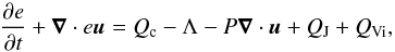 (1)where e is the internal energy per unit volume, u the velocity vector, P the gas pressure, and Qc the heating/cooling derived via the Spitzer thermal conduction along the magnetic field (Spitzer 1962). QJ represents the Joule heating, QVi is the viscous heating, and Λ the cooling or heating produced by the emission and absorption of radiation.
In the current work, we simulate the region from the solar convective zone up to the corona. The simulated volume starts 2.5 Mm below the photosphere and extends 14.3 Mm above the photosphere into the corona. We use periodic boundary condition in the horizontal x–y plane; in the vertical z-direction, the upper boundary is open, while the lower boundary is open, but remaining in hydrostatic equilibrium enabling convective flows to enter and leave the system. By controlling the entropy of the material flowing in through the bottom boundary, the effective temperature of the photosphere is kept roughly constant at 5.780 × 10³ K. The simulation box has a volume equal to 24 × 24 × 16.8 Mm3, which is resolved by 768 × 768 × 768 cells. Therefore, the horizontal grid spacing dx = dy = 31.25 km, whereas the vertical grid spacing varies to resolve the magnetic field, temperature, and pressure scale heights. Hence, the vertical spacing (dz) is approximately equal to 26.09 km in the photosphere, chromosphere and transition region, while it increases up to 165 km at the upper boundary in the corona. This simulation incorporates two strong magnetic regions of opposite polarity, which are connected with a magnetic structure with a loop-like shape. The magnetic field is initially set vertically at the bottom boundary and extrapolated to the whole atmosphere assuming potential field, while a horizontal 100 Gauss field is fed continuously in at the lower boundary producing random salt and pepper magnetic structures in the photosphere. Further details of the simulation setup can be found in Carlsson et al. (2016) which explains a similar setup, except the one describe in Carlsson et al. (2016) also includes the effects of non-equilibrium ionization of hydrogen.
To quantitatively study the effects of magnetic reconnection, we choose to analyze the joule heating term, which is calculated directly in Bifrost through Ohms law, using a non-constant electric resistivity. The resistivity (magnetic diffusivity) used in Bifrost code is numerical so as to ensure stability of the explicit code. The numerical resistivity is one of the diffusive terms used in the solution of the standard MHD partial differential equations. Bifrost employs a diffusive operator which is split into two major parts: a small global diffusive term and a location-specific diffusion term (Gudiksen et al. 2011). The numerical resistivity is constructed as a function of the grid size, so as to prevent current sheets from becoming unresolved; this gives rise to Reynolds numbers with order of magnitude larger than one. The exact formulation of the resistivity is described in Eq. (5) in Guerreiro et al. (2015). The electric resistivity is kept as low as possible, while still stabilizing the code. That means that the resistivity is not uniform in the computational box and it is larger than the microscopic resistivity throughout. The resistivity in the highest-current regions is consequently larger than everywhere else, but the sun also seems to have a method of increasing the resistivity locally, otherwise fast reconnection would not be possible (Biskamp 1986; Scholer 1989). How the sun is able to increase the electrical resistivity locally is not known, but several methods are possible, such as instabilities in the central current sheet leading to small-scale turbulence. How the resistivity behaves is unknown, except that it does increase in reconnection sites in the solar atmosphere. Bifrost therefore uses the most conservative value of the electric resistivity available, which is the value of the resistivity that keeps the code stable.
2.2. Identification method
We choose a region of interest (ROI), which starts from the lower corona, 3.28 Mm above the photosphere, where the temperature is on average equal to 1 MK, and extends up to the top of the simulation box. The volume of interest is resolved by 768 × 768 × 331 grid cells, spanning 24 × 24 × 9.5 Mm3.
Identifying locations with current sheets seems at first simple. Locating 3D volumes with high Joule heating should be easy enough, but it turns out not to be so simple. The problem we encounter is that the current sheets in 3D are generally not 2D flat structures, as the cartoon-like pictures of 2D reconnection would suggest, but much more complex. Often the “background” current level is higher in places with many current sheets, so it is not easy to separate one current sheet from another. That is in some ways similar to the problems experienced by observers, where the background is causing large problems for the interpretations. The method we have identified as the best is a powerful numerical tool, named “ImageJ”, used in medical imaging and bio-informatics to perform multi-dimensional image analysis (Ollion et al. 2013; Gul-Mohammed et al. 2014). ImageJ is an open-source tool in which users contribute by creating plugins for different purposes, making them available to everyone. In our case, we use the plugin “3D iterative thresholding” (also known as AGITA: Adaptive Generic Iterative Thresholding Algorithm, Gul-Mohammed et al. 2014), which first detects features for multiple thresholds, and then tries to build lineage between the detected features from one threshold to the next, and finally chooses the features that fall within the pre-specified criteria. Therefore, different features can be segmented at different thresholds. The thresholds tested here can be chosen based on three value parameters. The first parameter is the “step” parameter: the threshold increases by the specific input value (step) and features are identified between the previous threshold and the current one. The second parameter is “Kmeans”, in which a histogram is analyzed and clustered into the specific number of pre-specified number of classes. The last parameter is the “volume” parameter, for which the method tries to find a constant number of pixels between two thresholds for different threshold values in each step. In addition, for each lineage (same features segmented at different thresholds) the plugin allows various criteria to select the best identified feature. For instance, the “elongation” criterion chooses the most rounded features, the “volume” criterion chooses the largest features, and the “MSER” criterion chooses features with the smallest variation in number of pixels for different thresholds (i.e., the feature with the smallest number of pixels).
In our case, we first load our data, and then scale them from a 32-bit 3D image to 16-bit; instead of having single precision floats, we now have integers that scale from 0 to 65 535. The new image is scaled dynamically according to the upper and lower limits of the energy rate density. We then, use the iterative thresholding method using the “step” parameter equal to 50. The chosen step-parameter is based on a combination of making sure that the produced features do not change too much between successive thresholds, and still not being too computationally expensive to traverse the range from 0 to 65 535. We found a step size of 50 to be sufficient.
We also choose a minimum and maximum number of cells in a feature equal to 125 and 100 000 respectively; the minimum value is 125 because Bifrost uses 6th order differential and 5th order interpolation operators in a stagger grid where the computational stencil is six grid points. Choosing five grid cells in each direction is a very conservative choice, because the 6th-order operators should be able to resolve a peak with just three points. We also choose the volume criterion so that the method chooses the largest possible features, because we want to make sure that the method does not split features that are truly one feature, thereby changing the powerlaw distributions that are the goal of this investigation. The plugin then labels each feature with a specific number and we store each newly generated 3D image, each one labeled.
The method resolves only a fraction of the total joule heating of the specific snapshot calculated for the coronal region; this fraction is attributed to the identified “heating events”. The unresolved energy is considered to be a combination of unresolved features and background heating that is not correlated with impulsive events and effects of the imperfect method to separate features.
The background heating varies almost as much as its amplitude, and we have so far not been able to produce a method that would not disrupt the final statistics.
General characteristics can be derived after the identification of heating events. We calculate the spectral index α of the powerlaw distribution of the energy rate density and volume of the resolved objects using the method proposed by Aschwanden (2015). This method should counter the problems caused by factors such as the physical threshold of an instability changing for any physical reason, incomplete sampling, and contamination by event-unrelated background affecting the frequency of occurrence of small-scale events. The largest events will naturally be missing due to the limited volume and energy density of the ROI. The powerlaw fitting consequently has to take these limitations into account, and more free parameters then need to be included in the fit: 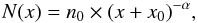 (2)where x denotes the specific quantity and n0 is a constant that depends on the total number of features (nf) in a range bounded from the maximum (x2) and minimum (x1) values
 ![Mathematical equation: \begin{equation} n_0 = n_{f}(1-\alpha)\left[x_2^{1-\alpha} - x_1^{1-\alpha}\right]^{-1}\!, \end{equation}](/articles/aa/full_html/2017/07/aa30748-17/aa30748-17-eq37.png) (3)where
(3)where  is the result of normalisation. Thus, we try to fit n0, α, and x0 of Eq. (2)via χ2 minimisation. The specific powerlaw fitting technique reduces the number of data points needed to fit the powerlaw, but in our case the difference between the identified events and the reduced ones is insignificant.
3. Results
The method mentioned in the previous section represents an effort to identify discrete heating events. We try to separate those events from other sources of heating that are not included in the Joule heating term.
Our method identifies initially large features, which are clusters of events and each comprised of more than 104 grid-cells. They are mostly located at the bottom of the corona, where most of the current sheets are formed, a result similar to what was observed by Gudiksen & Nordlund (2005). Features that have large horizontal cross-sections at the bottom of the corona lead to large volume when we perform the clustering method of Hoshen & Kopelman (1976). From looking at a 3D rendering of the large events and plotting the energy release along random lines throughout their volumes, it is clear that very large events are collections of many small events closely packed in space. Our method is clearly not able to identify features that are this closely packed.
The volume of the events is 4% of the total coronal volume and the total energy contained in all events is only 12% of the total Joule heating in the corona. The remaining 88% of joule heating is a combination of unsatisfied threshold criteria, which either do not satisfy the minimum resolution criterion or the method is unable to find the full extension of an event. The unresolved features with a volume less than 125 grid cells account for less than 0.1% of the total joule energy term in ROI, so the unresolved features are not a significant source of error.
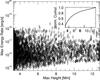 |
Fig. 1 Height of max energy rate for each identified feature with respect to the value of the maximum energy rate plotted in logarithmic scale; this height may be correlated with the height of event initiation. It is clear that the activity in the lower corona is higher than in the rest region. From the normalized cumulative plot we observe the same result: the biggest percentage of data points lays at the lower corona. |
Most of the heating events are located at the bottom of the corona, a fact that can be deduced from the density of features in Fig. 1. Both illustrations in Fig. 2 show that the heating events extend upward or hover in the corona. The analysis also shows that they usually have three shapes: fan-like, spine-like, and loop-like shapes. The same shapes have also been observed in simulations by Hansteen et al. (2015).
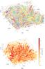 |
Fig. 2 Top: 3D rendering of 4136 identified features of the joule heating term, in which each color represents a different feature. Bottom: indentified features of joule heating in logarithmic scale. The energy output from the resolved features is 12% of the joule heating output, while the remaining 88% counts as background heating, numerical noise, and unresolved features. |
4. Statistical analysis
In Fig. 2 we are seeing the result of the heating events imprinted at a random moment in their life, and in the following we do statistics on these events.
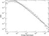 |
Fig. 3 Differential size distribution of the identified features’ energy rate in logarithmic scale representing N = 4136 identified features (diamonds). A powerlaw index α = 1.50 ± 0.02 is found, having goodness-of-fit χ2 = 14.28; the error is calculated as |

In Fig. 3, we plot the differential size distribution of released energy rate over logarithmic bin. The differential size distribution is defined as the number of features with sizes within a certain bin, divided by the bin size. To calculate the number of bins, we use the formula derived by Aschwanden (2015). The formula has the following form: 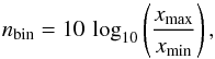 (4)where xmax and xmin are the maximum and minimum values in the data set, respectively. We notice that the distribution of the released energy rate follows a powerlaw function, which has the following form:
  (5)where the powerlaw index has a value of α = 1.5 ± 0.04. The error is calculated as
  , where NF = 1368 is the number of events and the powerlaw function is fitted within a range of released energy rate spanning from 2 × 10¹⁸ erg / s to 2 × 10²² erg / s.
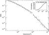 |
Fig. 4 Differential size distribution of the identified features’ volume in logarithmic scale. Two powerlaws are fitted to the data, which have slopes equal to α = 1.53 ± 0.03 with a goodness-of-fit χ2 = 3.43 and α = 2.53 ± 0.22 with a goodness-of-fit χ2 = 1.28. The first slope is fitted over 3542 data points in the range between 1.85 × 10²¹ and 1023 cm3, whereas the second over 137 data points in the range between 1022 and 1024 cm3. In the right corner the cumulative of the resolved volume is plotted, that is, N( <x) = f(x). |
The volume of events is also important. In Fig. 4, we plot the differential size distribution of volume, along with the fitted powerlaw function. What we find is two spectral indices αV = 1.53 ± 0.03 within a range between 1021 and 1023 cm3 and αV = 2.53 ± 0.22 within a range between 1023 and 2 × 1024 cm3. To find which scale of events’ volume is the most important in terms of space filling, we plot in Fig. 4 the cumulative size distribution of this size. It seems that large-scale events, that is, structures larger than 1023 cm3, which correspond to 137 events occupy 40% of the resolved volume in the ROI.
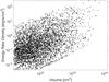 |
Fig. 5 Energy release rate over volume versus volume of identified features in logarithmic scale. |
We also check for any correlation between volume and energy release per volume. Figure 5 depicts the two quantities plotted against each other for all identified events. The two quantities seem not to have any clear correlation. Features of any volume span more than three orders of magnitude, and features with any energy rate density span two and half orders of magnitude in volume.
To further test the connection between volume and the energy release rate per volume, we perform Spearman’s rank and Pearson linear correlation. The rank correlation showed a merely bad global correlation, that is, ρ = 0.4 (this correlation varies between 0 and 1, smaller values indicate good rank correlation), whereas there is very weak linear correlation (i.e., ρ = 0.53) between the two quantities (Pearson correlation varies between –1 and 1).
Figure 1 shows the maximum energy release rate of each event as a function of the height at which the specific maximum energy release is located. If we assume that the location of the maximum energy release is the location where an event is initially triggered, then the plot suggests possible height of instability triggering.
From the normalized cumulative plot, and from the plot itself, we observe that the lower corona contains not only most of the heating events but also the most energetic ones. Almost 40% of the total number of events are located between 3 and 4 Mm above the photosphere. The number of events in larger heights up to 14 Mm above the photosphere is distributed almost evenly while the maximum energy release rate drops with height. Therefore, the heating in the lower corona is larger than in the upper layers, a trend also observed by Gudiksen & Nordlund (2002).
5. Disussion and conclusions
This paper discusses the implementation of a multi-thresholding technique implemented in 3D MHD simulation aiming to identify three dimensional joule heating events at a randomly selected snapshot from a numerical simulation of the solar corona.
Using the Bifrost code, we simulate the solar environment enabling us to identify events in the modeled solar corona with high resolution. Those events release power that spans almost four orders of magnitude starting from 1017 erg / s , and has volume spanning three orders of magnitude starting from 1021 cm3. The events follow a powerlaw over many orders of magnitude just like many other self-organized critical systems, suggesting that the formation of these structures share the same physical mechanism that scale in the energy and volume regimes.
The outcome is the result of the stochastic nature of magnetic reconnections’ ability to release energy stored in the magnetic field, when it reaches a threshold. The stochastic nature originates from the fact that magnetic reconnection triggers an instability in which a random fraction of the energy stored in the magnetic field is released. In some cases observations show that this system appears to have memory of previous energy releases as magnetic reconnection events are sometimes observed to happen at the same location within a short amount of time, such as in homologous flares (Fokker 1967). This is, in our opinion, caused by the stochastic nature of the total energy release. If the energy released is relatively small compared to the surplus energy stored in the magnetic field at a specific location, then the fact that energy is released might produce conditions where only a small increase in the stored energy can lead to yet another energy release.
We find that there is no global linear relation between energy release and volume, and the Spearman’s rank correlation shows a merely bad correlation.
Generally, the heating is mostly concentrated at the bottom of the corona and gradually drops with height because the magnetic field magnitude also drops with height; a fact that was pointed out and explained by Gudiksen & Nordlund (2002). A consequence of the distribution is that energetic events are more likely to be generated in the lower corona.
The differential size distribution of released energy rate and volume follow a powerlaw distribution. What we find are slopes that favor the release of energy in large events.
As illustrated in Fig. 2, the method can resolve large structures into smaller ones and identify where most of the heating occurs locally even though some of the energy is no longer in identified events. The unresolved energy might be attributed to two categories of mechanism; technical and physical. In the first category, unsatisfied thresholding criteria, unresolved features or numerical heating due to noise have an impact on identifying real heating events. The unresolved energy could be due to heating from other sources, such as MHD waves that distort the magnetic field, or remnants of current sheets after energetic events that burn slowly (Janvier et al. 2014). Finding dissipating MHD wave modes in this snapshot is beyond the scope of this work.
Our method cannot identify all the energy released as events. If the large part of the total Joule heating, which is not identified as events in this work, actually is small events, then they would be added to the low-energy tail of our powerlaw plots and would then increase α. Without any evidence for this being the case, we cannot say if the remaining 88% of the total Joule heating is in the form of small events. If they were, we would most likely see a powerlaw index being close to or above two since most of the energy would then be delivered through small events. We are at the moment considering paths to establish this.
The time evolution of the heating events is another unknown which is beyond the scope of this work. What we analyze is the fingerprints of heating events at a specific time. We do not take into account the lifetime of the events. Several authors have reported lifetimes of small and large events not being the same or even the increase and decrease of heating events being dissimilar (Lee et al. 1993; Klimchuk 2006; Morales & Charbonneau 2008; Christe et al. 2008; Hannah et al. 2011). Therefore, the duration of the heating events, which is usually considered in observations, may affect the calculated powerlaw indices when energy release is studied, instead of energy rate as we do in the current analysis.
We are able to extract information about the released energy rate and volume ranges of identified events. The smallest event we identify is significantly smaller than the lower limit for what can be observed. Even though we have much more information available through our numerical model, it is interesting how similar the problems of identifying events are from an observational and numerical stand point. The problems arise due to different limitations.
The results of our method can be compared with similar studies that also investigate the joule heating term in simulations or observations using different methods for identifying heating events. For example, Bingert & Peter (2013) divide their simulation box into cubes of identical sizes and the temporal dimension into constant time-intervals and finally they count the energy released in those boxes. Moraitis et al. (2016) use a partitional clustering code. The code uses the Manhattan distance to group 3D voxels above a threshold into clusters. Guerreiro et al. (2015) find all the local maxima of joule heating terms in a 3D MHD simulation. They then try to identify 3D events by locating the minimum value above a threshold, the threshold is defined as a constant fraction of the local maximum value. Regardless of how each study defines a heating event, all authors find that the released energy follows a power-law distribution with slopes flatter than two. Interestingly, Bingert & Peter (2013) also find that heating in the corona drops with height. It is remarkable that our power-law index for the rate of energy release and that of the energy release found by Bingert & Peter (2013) are very similar. In addition, our power-law of volumes at the right part of the knee is almost identical with that found by the same authors for the same range of volumes. While being able to identify smaller structures with our method, we see that the slope becomes flatter.
Our identification method is a first step towards finding the powerlaw exponent of the distribution of heating events. The exponents we report on here seem to be only lower limits, and in future work we will attempt to solve some of the problems
mentioned, by looking at time evolution and the observational effects of the identified heating events.
References
- Aschwanden, M. J. 2015, ApJ, 814, 19 [NASA ADS] [CrossRef] [Google Scholar]
- Aschwanden, M. J., & Shimizu, T. 2013, ApJ, 776, 132 [NASA ADS] [CrossRef] [Google Scholar]
- Aschwanden, M. J., Crosby, N. B., Dimitropoulou, M., et al. 2016, Space Sci. Rev., 198, 47 [NASA ADS] [CrossRef] [Google Scholar]
- Bak, P., Tang, C., & Wiesenfeld, K. 1988, Phys. Rev. A, 38, 364 [NASA ADS] [CrossRef] [MathSciNet] [PubMed] [Google Scholar]
- Benz, A. O., & Krucker, S. 2002, ApJ, 568, 413 [NASA ADS] [CrossRef] [Google Scholar]
- Bingert, S., & Peter, H. 2013, A&A, 550, A30 [NASA ADS] [CrossRef] [EDP Sciences] [Google Scholar]
- Biskamp, D. 1986, in Magnetic Reconnection and Turbulence, eds. M. A. Dubois, D. Grésellon, & M. N. Bussac, 19 [Google Scholar]
- Carlsson, M., & Leenaarts, J. 2012, A&A, 539, A39 [NASA ADS] [CrossRef] [EDP Sciences] [Google Scholar]
- Carlsson, M., & Stein, R. F. 2002, ApJ, 572, 626 [NASA ADS] [CrossRef] [Google Scholar]
- Carlsson, M., Hansteen, V. H., de Pontieu, B., et al. 2007, PASJ, 59, S663 [Google Scholar]
- Carlsson, M., Hansteen, V. H., Gudiksen, B. V., Leenaarts, J., & De Pontieu, B. 2016, A&A, 585, A4 [NASA ADS] [CrossRef] [EDP Sciences] [Google Scholar]
- Christe, S., Hannah, I. G., Krucker, S., McTiernan, J., & Lin, R. P. 2008, ApJ, 677, 1385 [NASA ADS] [CrossRef] [Google Scholar]
- Fokker, A. D. 1967, Sol. Phys., 2, 316 [NASA ADS] [CrossRef] [Google Scholar]
- Galsgaard, K., & Nordlund, Å. 1996, J. Geophys. Res., 101, 13445 [NASA ADS] [CrossRef] [Google Scholar]
- Georgoulis, M. K., & Vlahos, L. 1996, ApJ, 469, L135 [NASA ADS] [CrossRef] [Google Scholar]
- Gold, T. 1964, The physics of Solar Flares, Proc. AAS-NASA Symp., ed. W. Hess, 389 [Google Scholar]
- Gudiksen, B. V., & Nordlund, Å. 2002, ApJ, 572, L113 [Google Scholar]
- Gudiksen, B. V., & Nordlund, Å. 2005, ApJ, 618, 1020 [NASA ADS] [CrossRef] [Google Scholar]
- Gudiksen, B. V., Carlsson, M., Hansteen, V. H., et al. 2011, A&A, 531, A154 [NASA ADS] [CrossRef] [EDP Sciences] [Google Scholar]
- Guerreiro, N., Haberreiter, M., Hansteen, V., & Schmutz, W. 2015, ApJ, 813, 61 [NASA ADS] [CrossRef] [Google Scholar]
- Gul-Mohammed, J., Arganda-Carreras, I., Andrey, P., Galy, V., & Boudier, T. 2014, BMC Bioinformatics, 15, 9 [CrossRef] [Google Scholar]
- Hannah, I. G., Hudson, H. S., Battaglia, M., et al. 2011, Space Sci. Rev., 159, 263 [NASA ADS] [CrossRef] [Google Scholar]
- Hansteen, V., Guerreiro, N., De Pontieu, B., & Carlsson, M. 2015, ApJ, 811, 106 [NASA ADS] [CrossRef] [Google Scholar]
- Hoshen, J., & Kopelman, R. 1976, Phys. Rev. B, 14, 3438 [NASA ADS] [CrossRef] [Google Scholar]
- Hudson, H. S. 1991, Sol. Phys., 133, 357 [Google Scholar]
- Janvier, M., Aulanier, G., Pariat, E., & Demoulin, P. 2013, A&A, 555, A77 [NASA ADS] [CrossRef] [EDP Sciences] [Google Scholar]
- Janvier, M., Aulanier, G., Bommier, V., et al. 2014, ApJ, 788, 60 [NASA ADS] [CrossRef] [Google Scholar]
- Klimchuk, J. A. 2006, Sol. Phys., 234, 41 [NASA ADS] [CrossRef] [Google Scholar]
- Lee, T. T., Petrosian, V., & McTiernan, J. M. 1993, ApJ, 412, 401 [NASA ADS] [CrossRef] [Google Scholar]
- Leenaarts, J., Carlsson, M., Hansteen, V., & Rouppe van der Voort, L. 2009, ApJ, 694, L128 [NASA ADS] [CrossRef] [Google Scholar]
- Low, B. C. 1990, ARA&A, 28, 491 [NASA ADS] [CrossRef] [Google Scholar]
- Lu, E. T., & Hamilton, R. J. 1991, ApJ, 380, L89 [NASA ADS] [CrossRef] [Google Scholar]
- Moraitis, K., Toutountzi, A., Isliker, H., et al. 2016, A&A, 596, A56 [NASA ADS] [CrossRef] [EDP Sciences] [Google Scholar]
- Morales, L., & Charbonneau, P. 2008, ApJ, 682, 654 [NASA ADS] [CrossRef] [Google Scholar]
- Morales, L., & Charbonneau, P. 2009, ApJ, 698, 1893 [NASA ADS] [CrossRef] [Google Scholar]
- Ollion, J., Cochennec, J., Loll, F., Escudé, C., & Boudier, T. 2013, Bioinformatics, 29, 1840 [Google Scholar]
- Parker, E. N. 1972, ApJ, 174, 499 [NASA ADS] [CrossRef] [Google Scholar]
- Parker, E. N. 1983a, ApJ, 264, 642 [NASA ADS] [CrossRef] [Google Scholar]
- Parker, E. N. 1983b, ApJ, 264, 635 [NASA ADS] [CrossRef] [Google Scholar]
- Parker, E. N. 1988, ApJ, 330, 474 [Google Scholar]
- Parnell, C. E., & Jupp, P. E. 2000, ApJ, 529, 554 [NASA ADS] [CrossRef] [Google Scholar]
- Priest, E. R., & Forbes, T. G. 2002, A&ARv, 10, 313 [NASA ADS] [CrossRef] [Google Scholar]
- Priest, E. R., & Pontin, D. I. 2009, Phys. Plasmas, 16, 122101 [NASA ADS] [CrossRef] [Google Scholar]
- Priest, E. R., & Titov, V. S. 1996, Philos. Trans. Roy. Soc. Lond. Ser. A, 354, 2951 [Google Scholar]
- Scholer, M. 1989, J. Geophys. Res., 94, 8805 [NASA ADS] [CrossRef] [Google Scholar]
- Spitzer, L. 1962, Physics of Fully Ionized Gases (New York: Interscience) [Google Scholar]
- Viall, N. M., & Klimchuk, J. A. 2011, ApJ, 738, 24 [Google Scholar]
All Figures
|
Fig. 1 Height of max energy rate for each identified feature with respect to the value of the maximum energy rate plotted in logarithmic scale; this height may be correlated with the height of event initiation. It is clear that the activity in the lower corona is higher than in the rest region. From the normalized cumulative plot we observe the same result: the biggest percentage of data points lays at the lower corona. |
| In the text | |
|
Fig. 2 Top: 3D rendering of 4136 identified features of the joule heating term, in which each color represents a different feature. Bottom: indentified features of joule heating in logarithmic scale. The energy output from the resolved features is 12% of the joule heating output, while the remaining 88% counts as background heating, numerical noise, and unresolved features. |
| In the text | |
|
Fig. 3 Differential size distribution of the identified features’ energy rate in logarithmic scale representing N = 4136 identified features (diamonds). A powerlaw index α = 1.50 ± 0.02 is found, having goodness-of-fit χ2 = 14.28; the error is calculated as |
| In the text | |
|
Fig. 4 Differential size distribution of the identified features’ volume in logarithmic scale. Two powerlaws are fitted to the data, which have slopes equal to α = 1.53 ± 0.03 with a goodness-of-fit χ2 = 3.43 and α = 2.53 ± 0.22 with a goodness-of-fit χ2 = 1.28. The first slope is fitted over 3542 data points in the range between 1.85 × 10²¹ and 1023 cm3, whereas the second over 137 data points in the range between 1022 and 1024 cm3. In the right corner the cumulative of the resolved volume is plotted, that is, N( <x) = f(x). |
| In the text | |
|
Fig. 5 Energy release rate over volume versus volume of identified features in logarithmic scale. |
| In the text | |
Current usage metrics show cumulative count of Article Views (full-text article views including HTML views, PDF and ePub downloads, according to the available data) and Abstracts Views on Vision4Press platform.
Data correspond to usage on the plateform after 2015. The current usage metrics is available 48-96 hours after online publication and is updated daily on week days.
Initial download of the metrics may take a while.