| Issue |
A&A
Volume 601, May 2017
|
|
|---|---|---|
| Article Number | A27 | |
| Number of page(s) | 8 | |
| Section | Galactic structure, stellar clusters and populations | |
| DOI | https://doi.org/10.1051/0004-6361/201630253 | |
| Published online | 24 April 2017 | |
Population synthesis to constrain Galactic and stellar physics
I. Determining age and mass of thin-disc red-giant stars
Institut UTINAM, CNRS UMR 6213, Univ. Bourgogne Franche-Comté, OSU THETA Franche-Comté-Bourgogne, Observatoire de Besançon, BP 1615, 25010 Besançon Cedex, France
e-mail: This email address is being protected from spambots. You need JavaScript enabled to view it.
Received: 14 December 2016
Accepted: 5 February 2017
Abstract
Context. The cornerstone mission of the European Space Agency, Gaia, together with forthcoming complementary surveys (CoRoT, Kepler, K2, APOGEE, and Gaia-ESO), will revolutionize our understanding of the formation and history of our Galaxy, providing accurate stellar masses, radii, ages, distances, as well as chemical properties for a very large sample of stars across different Galactic stellar populations.
Aims. Using an improved population synthesis approach and new stellar evolution models we attempt to evaluate the possibility of deriving ages and masses of clump stars from their chemical properties.
Methods. A new version of the Besançon Galaxy models (BGM) is used in which new stellar evolutionary tracks are computed from the stellar evolution code STAREVOL. These provide global, chemical, and seismic properties of stars from the pre-main sequence to the early-AGB. For the first time, the BGM can explore the effects of an extra-mixing occurring in red-giant stars. In particular we focus on the effects of thermohaline instability on chemical properties as well as on the determination of stellar ages and masses using the surface [C/N] abundance ratio.
Results. The impact of extra-mixing on 3He, 12C/13C, nitrogen, and [C/N] abundances along the giant branch is quantified. We underline the crucial contribution of asteroseismology to discriminate between evolutionary states of field giants belonging to the Galactic disc. The inclusion of thermohaline instability has a significant impact on 12C/13C, 3He as well as on the [C/N] values. We clearly show the efficiency of thermohaline mixing at different metallicities and its influence on the determined stellar mass and age from the observed [C/N] ratio. We then propose simple relations to determine ages and masses from chemical abundances according to these models.
Conclusions. We emphasize the usefulness of population synthesis tools to test stellar models and transport processes inside stars. We show that transport processes occurring in red-giant stars should be taken into account in the determination of ages for future Galactic archaeology studies.
Key words: Galaxy: stellar content / Galaxy: abundances / asteroseismology / stars: evolution / stars: abundances / Galaxy: evolution
© ESO, 2017
1. Introduction
Galactic archaeology explores the formation and evolution of our Galaxy using the chemical properties, kinematics, and their dependency on age, of different stellar populations (Freeman & Bland-Hawthorn 2002; Turon et al. 2008). In this context, the determination of accurate stellar distances and ages along the Galactic disc is crucial to improving our understanding of the Milky Way.
The Gaia space mission provided astrometry for more than two million stars and photometry for one billion stars, with typical uncertainties of about 0.3 mas for the positions and parallaxes, and about 1 mas/yr for the proper motions (first data release, Gaia Collaboration 2016). Asteroseismology data of red-giant stars observed by the space missions CoRoT (Baglin & Fridlund 2006), Kepler (Gilliland et al. 2010), and K2 provide crucial constraints on the stellar properties such as masses, radii, and evolutionary states (e.g. Stello et al. 2008; Mosser et al. 2012b; Bedding et al. 2011; Vrard et al. 2016), on the internal rotation profile (e.g. Mosser et al. 2012a; Beck et al. 2012), as well as on the properties of helium ionization regions (Miglio et al. 2010). Thanks to asteroseismology, masses of red-giant stars can be directly related to stellar interior physics and stellar evolution (Lebreton et al. 2014a,b) allowing one to determine ages, without being limited to surface properties. Seismic data collected for more than 20 000 red-giant stars belonging to the Galactic-disc populations represent a huge sample to constrain stellar and Galactic physics (Miglio et al. 2013; Anders et al. 2016). A broad effort is ongoing with large spectroscopic surveys such as APOGEE (Majewski et al. 2015; SDSS Collaboration 2016), ESO-Gaia (Gilmore et al. 2012), RAVE (Steinmetz et al. 2006), SEGUE (Yanny et al. 2009), LAMOST (Cui et al. 2012), HERMES (Ackerstaff et al. 1998), and for the future with WEAVE, 4MOST, and MOONS, from which stellar parameters, radial velocities, and detailed chemical abundances can be measured for CoRoT, Kepler, and K2 targets.
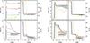 |
Fig. 1 Theoretical evolution of 3He and carbon isotopic ratio at the stellar surface as a function of surface gravity for stellar models of: left panels various masses (1.0; 1.2; 1.5; 1.8; 3.0 M⊙ represented by a black, red, blue, green and orange solid line, respectively) at Z = 0.04; right panels various metallicities ([Fe/H] = 0.5; 0; −0.23; −0.54; −2.14 represented by a black, red, blue, green and orange solid line, respectively) at M = 1.2 M⊙. These models include the effects of thermohaline instability (bottom panels) and following standard evolution (top panels). These tracks are shown from the main sequence up to the early-AGB. |
To exploit their full potential, it is crucial to perform a combined analysis of these different kinds of observations. The population synthesis approach is a powerful tool for such analysis, allowing the computation of mock catalogues under various model hypothesis, and to statistically compare these simulated catalogues with any type of large survey data. The Besançon Galaxy model (BGM) is a stellar population synthesis model (Robin et al. 2003; Czekaj et al. 2014) intended to meld the formation and evolution scenarios of the Galaxy, stellar formation and evolution theory, and models of stellar atmospheres, as well as dynamical constraints, in order to make a consistent picture of the Galaxy in comparison with available observations (photometry, asteroseismology, astrometry, and spectroscopy) at different wavelengths.
To benefit from the combination of recent asteroseismic and spectroscopic surveys, we updated the evolutionary tracks that are used as inputs in the BGM. These stellar evolution models are computed with the code STAREVOL (e.g. Lagarde et al. 2012a), which follows the global, chemical, and seismic properties of stars all along their evolution. This is done from the pre-main sequence (along the Hayashi track) to the early-asymptotic giant branch (early-AGB). These models include the effects of different transport processes such as thermohaline instability (discussed in this paper).
The aim of this series of papers is to investigate the impacts of different hydrodynamic processes that occur inside the stars on the chemical properties of Galactic stellar populations. In the context of the interpretation of large spectroscopic surveys such as APOGEE or Gaia-ESO, we will perform comparisons between theoretical synthetic populations and spectroscopic surveys in forthcoming papers (Lagarde et al., in prep., Paper II). In this paper, we focus on presenting and discussing the implementation of stellar evolution models that include the effects of thermohaline instability on global, chemical, and seismic properties, in the BGM. We discuss the determination of stellar ages and masses from the [C/N] ratio. We plan to focus on the effects of rotation and the implementation of different prescriptions for thermohaline instability on stellar ages and chemical properties in a separate forthcoming paper (Paper III). In Sect. 2 we present the input physics of our stellar evolution models and briefly recall the impacts of thermohaline instability on the chemical properties of giant stars. The BGM is presented in Sect. 3, while in Sect. 4 we present synthetic stellar populations, taking into account the effects of thermohaline mixing or following the standard prescription. We also present the new quantities that can be simulated by the BGM. In Sect. 5, we discuss the determination of stellar ages and masses from the surface carbon and nitrogen abundances, and we provide relations for three metallicity ranges. We conclude and explore some perspectives in Sect. 6.
2. Stellar evolution models
2.1. Description of stellar evolution models
Stellar evolution models.
Stellar evolution models are computed with the code STAREVOL (e.g. Lagarde et al. 2012b) for a range of masses between 0.6 M⊙ and 6.0 M⊙ at five metallicities Z = 0.04 ([Fe/H] = 0.51), Z = 0.0134 ([Fe/H] = 0), Z = 0.008 ([Fe/H] = −0.23), Z = 0.004 ([Fe/H] = −0.54), and Z = 0.0001 ([Fe/H] = −2.14). These models are computed from the pre-main sequence to the early-AGB phase. We use the same main physical ingredients that are used and fully described in Lagarde et al. (2012a), except for:
-
the solar mixture, that comes from Asplundet al. (2009);
-
the treatment of convection, that is based on a classical mixing length formalism with αMLT= 1.6264 recovered from solar-calibrated models that include neither atomic diffusion nor rotation.
As discussed in Lagarde et al. (2012a), these stellar evolution models follow the global asteroseismic properties using the scaling relations and asymptotic relations (Tassoul 1980), that is, the large frequency separation, the frequency corresponding to the maximum oscillation power, the asymptotic period spacing of g-modes, and different acoustic radii.
To quantify the effects of transport processes on the chemical properties of stellar populations in our Galaxy, we computed stellar evolution models assuming: (1) standard models (no mixing mechanism other than convection); (2) models that include the effects of thermohaline instability induced by 3He-burning. This instability develops as long thin fingers whose aspect ratio is consistent with predictions by Ulrich (1972) and with laboratory experiments (Krishnamurti 2003). Although the efficiency of thermohaline instability in stellar interiors is still discussed in the literature by hydrodynamical simulations (Denissenkov 2010; Traxler et al. 2011; Prat et al., in prep.), we adopt an aspect ratio equal to five, which might correspond to the maximum efficiency of this instability.
As discussed by Charbonnel & Lagarde (2010) and Angelou et al. (2011; 2012), this mechanism has a crucial effect on the surface chemical properties of red-giant branch stars. Its effect is consistent with most spectroscopic observations of low-mass and intermediate-mass stars, especially in reproducing the low-12C/13C and the [C/N] ratio in open clusters (e.g. Tautvaišienė et al. 2016, 2015, 2013; Drazdauskas et al. 2016; Mikolaitis et al. 2010; Smiljanic et al. 2009) as well as in CoRoT targets (Morel et al. 2014; Lagarde et al. 2015). It has also a very significant impact on the chemical evolution of light elements in the Milky Way (Lagarde et al. 2011) allowing the resolution of the long-standing “3He-problem” in our Galaxy (Lagarde et al. 2012b). In the following section, we briefly describe the evolution of stars and present the effects of thermohaline mixing on the surface abundances of 3He and carbon isotopic ratio drawing the stellar evolution.
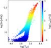 |
Fig. 2 Large separation, Δν, as a function of the effective temperature, Teff, for synthetic population computed with the BGM. Colours indicate the νmax, the frequency at which the power spectrum is maximum. |
2.2. Chemical evolution of low- and intermediate-mass giant stars
2.2.1. Standard evolution
Figure 1 presents the theoretical evolution of Helium-3 and carbon isotopic ratio for different initial masses and metallicities from the main sequence to the early-AGB. After the main sequence, a star experiences core contraction to increase its central temperature, then evolves rapidly toward the red giant branch (RGB). During this phase, called the “sub giant branch” (SGB) when the stars cross the HR diagram almost horizontally, the convective envelope grows in mass and deepens inside the star. This is the first dredge-up, where the convective envelope is diluted with hydrogen-processed material, inducing changes of the surface abundances. This episode occurs at higher luminosity when the metallicity decreases as well as when the stellar mass increases. The surface mass fractions of 7Li, 9Be, 12C, and 18O decrease while those of 3He, 4He, 13C, 14N, and 17O increase, implying a decrease at the surface of the isotopic ratios 12C/13C and 12C/14N. Figure 1 clearly shows the signature of this episode (e.g. at log(g) ~ 3.8 for 1.2 M⊙).
As shown by Charbonnel (1994), the first dredge-up efficiency (in terms of maximum depth of the convective envelope) decreases with decreasing metallicity. For a given stellar mass, Fig. 1 (right panel) shows that the depletion of 12C/13C and the increase of 3He begin at lower gravity when the metallicity decreases. The chemical variations during the first dredge-up depend on the initial stellar mass as well as on the metallicity. For a given metallicity, when the initial stellar mass increases, Fig. 1 (left panels) shows that the post dredge-up values of the carbon isotopic ratio and 3He decrease. This dependence is true for 12C/14N, as well as for oxygen isotopic ratios. This is due to the convective envelope reaching deeper regions during the first dredge-up. From the sub giant branch to the RGB tip, the temperature at the base of the convective envelope is always insufficient to activate nuclear reactions. As a consequence, in standard models (top panels of Fig. 1) the only change in surface abundances is due to the first dredge-up on the SGB; after this episode the surface abundances remain constant along the RGB once the convective envelope recedes and until the second dredge-up occurs at the end of the helium burning phase.
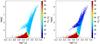 |
Fig. 3 Surface gravity as a function of effective temperature for synthetic populations computed with the BGM including the effects of thermohaline instability (right panel) or not (left panel). The colour code represents the carbon isotopic ratio at the surface of stars in the thin disc. |
2.2.2. Thermohaline instability during the RGB
Thermohaline mixing has recently been flagged as the main mechanism that can govern the photospheric chemical composition of low-mass bright giant stars (Charbonnel & Zahn 2007; Charbonnel & Lagarde 2010). In such stars, thermohaline instability is a double-diffusive instability induced by the molecular weight inversion created by the 3He(3He,2p)4He reaction in the external region of the hydrogen-burning shell (Eggleton et al. 2006, 2008). As discussed by Charbonnel & Zahn (2007) and Charbonnel & Lagarde (2010), this instability is expected to set in after the first dredge-up when the star reaches the RGB-bump (at log(g) ~ 2.5 on bottom panels of Fig. 1). In terms of stellar structure, the RGB bump corresponds to the moment when the hydrogen-burning shell encounters the chemical discontinuity created by the convective envelope at its maximum penetration during the first dredge-up. When the hydrogen burning shell (which provides the stellar luminosity on the RGB) reaches the H-rich previously mixed zone, the corresponding decrease in molecular weight of the H-burning layers induces a drop in the total stellar luminosity, creating a bump in the luminosity function (i.e. Fusi Pecci et al. 1990; Charbonnel 1994; Charbonnel et al. 1998).
Thermohaline mixing induces a decrease of 3He at the stellar surface after the RGB-bump. The chemical elements 13C and 14N diffuse outwards, while 12C diffuses inwards (see for more details Charbonnel & Lagarde 2010), implying a decrease of 12C/13C and [C/N]. The efficiency of thermohaline instability decreases when the stellar mass or stellar metallicity increase (see Fig. 1). In addition, thermohaline mixing induces a slight decrease of 3He (Lagarde et al. 2011) and increase of nitrogen at lower metallicity during the central helium burning before the second dredge-up episode. Thermohaline instability does not change the evolutionary tracks in the HR-diagram and has no impact on stellar ages because it has no significant effect on the stellar structure.
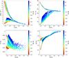 |
Fig. 4 Surface abundance of 3He (in mass fraction, top-left panel), 12C/13C (top-right panel), [C/Fe] (bottom-left panel), and [N/Fe] (bottom-right panel) as a function of stellar mass for synthetic thin disc computed with the BGM. Stars have been selected to be in the clump according to their ΔΠℓ = 1. The colour code represents the metallicity of stars. Simulations including or not the effects of thermohaline instability are represented by colour-dots and crosses respectively. |
3. The Besançon Galaxy model
The BGM is a model using the population synthesis approach that simulates observations of the sky with errors and biases. It is based on assumptions and a scenario for Galaxy formation and evolution that reflect the present knowledge about the Milky Way. Four stellar populations are considered: a thin disc, a thick disc, a bar, and a halo, with each stellar population having a specific density distribution. The stellar content of each population is modelled through an initial mass function (IMF) and a star formation history (SFH), which can differ from one population to another. To compute the stellar distribution at a given time, the stars generated by these IMFs and SFHs follow evolutionary tracks. When they have reached their final age (the present time) their astrophysical parameters (mass, age, Teff, log(g), metallicity, abundances) are stored and used to compute their observational properties, using atmosphere models, and assuming a 3D extinction map describing the interstellar extinction they suffer. A dynamical model is used to compute radial velocities and proper motions. In the simulations presented here, we make use of the 3D extinction map from Marshall et al. (2006).
For the time being, the metallicity of each star is the initial metallicity of the gas when it was born, which is estimated assuming a time dependent metallicity from Haywood (2008), and a radial metallicity gradient of −0.7 dex/kpc. In the future a proper chemical evolution model will be incorporated.
The model takes into account the stellar binarity by generating secondary components at their birth, assuming a binarity probability depending on mass (see Czekaj et al. 2014 for more details). Then, according to the estimated spatial resolution of the observations to simulate, stars in systems are merged or not (that is, their fluxes are added if the stars are too close, projected on the plane of the sky).
In the present version of the model, only the thin disc is modelled this way, while the thick disc, bar, and stellar halo are generated using a Hess diagram computed from a fixed evolutionary scheme as described in Robin et al. (2003), which does not yet take into account binarity. The stellar densities in different regions of the Galaxy are modulated by density laws for each population, which are given in detail in Robin et al. (2003) for the thin disc, Robin et al. (2012) for the bar, and Robin et al. (2014) for the thick disc and halo.
In the model version presented here, we use the evolutionary tracks described in Sect. 2, instead of the Padova tracks used in Czekaj et al. (2014), from which surface abundances and asteroseismic parameters are computed for each simulated star. For stars of mass lower than 0.6 solar mass, Chabrier & Baraffe (1997) evolutionary tracks are still used, although those new properties are not computed yet.
4. Simulations of synthetic populations
As discussed in Part 2 and in the literature (Palacios et al. 2006; Lagarde et al. 2012a; Bossini et al. 2015), transport processes occurring in stellar interiors have significant impact on global (e.g. luminosity, effective temperature, age), chemical, and seismic properties. Population syntheses are powerful tools to study these processes using survey data. In the context of our study, we discuss the impact of thermohaline mixing on the properties of thin disc giants observed by asteroseismic and spectroscopic surveys. We shall consider in a future paper the thick disc population, which differs from the thin disc by its [α/Fe] abundance ratio. For the present study we only consider stellar models according to solar α-abundance (i.e. [α/Fe] = 0). In order to estimate the impact of these stellar models on the populations observed, we performed simulations with the BGM using these new stellar evolutionary tracks and assuming the IMF and SFR given in Czekaj et al. (2014). Simulations are performed, for example, in the Kepler field. They provide astrophysical parameters, asteroseismic properties, and surface abundances for 54 stable and unstable species. We study in this section the impact this new model on the properties of the simulated fields.
4.1. Asteroseismic properties
The detection of solar-like oscillations by the space missions CoRoT and Kepler provides powerful constraints on the stellar mass and radius of giants stars. With the asymptotic period spacing of gravity modes, these observations provide information on stellar structure (Mosser et al. 2012b; Lagarde et al. 2012a), as well as constraints on transport processes (Lagarde et al. 2016). Using the scaling relations (Tassoul 1980; Mosser et al. 2010; Belkacem et al. 2011), the asteroseismic parameters of large separation, Δν, and frequency of maximum oscillation power, νmax are directly related to stellar radii and masses: 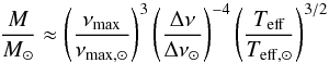 (1)
(1)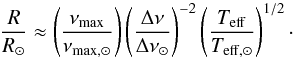 (2)Solar reference values are Δν⊙ = 135.1 μHz; νmax, ⊙ = 3090 μHz, and Teff, ⊙ = 5777 K. Miglio (2012) and Mosser et al. (2013) proposed a relative correction to the scaling relations between red clump and RGB stars. This should affect the mass and radius determinations of clump stars up to ~10% and ~6% respectively. Different temperature scales have been tested in Miglio (2012) and agree within the quoted uncertainty range.
The population synthesis provides the seismic properties such as the large separation, the frequency with the maximum amplitude, or the asymptotic period spacing of g-modes for stars in the thin disc (see Fig. 2). It is well known that the age of giant stars can be approximated by their lifetime on the main sequence, which depends on the stellar mass and metallicity. In addition, asteroseismology provides accurate stellar radii and thus allows the determination of distances. These observations of giants belonging to the different populations of the Milky Way provide additional constraints to study the formation and evolution of our Galaxy (Miglio et al. 2013). To fully exploit the potential of these observations, it is crucial to combine them with spectroscopic surveys allowing the following of the chemical properties of the stars within the different stellar populations.
4.2. Surface chemical properties
Figure 3 shows the evolution of the carbon isotopic ratio along the log(g) vs. Teff diagram in a simulation computed with the BGM. This figure clearly shows the impact of thermohaline instability on the 12C/13C. The brighter-RGB and clump stars have a lower 12C/13C at the surface when thermohaline instability is included.
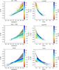 |
Fig. 5 Surface abundance of [C/N] as a function of stellar ages (left panels) and stellar masses (right panels), colour-coded by metallicity, for a synthetic thin disc computed with the BGM. Stars have been selected to be in the clump according to their ΔΠℓ = 1, as well as before and after the RGB-bump according to their log(g) values. Simulations including or not the effect of thermohaline instability are shown as colour-dots and grey crosses respectively. |
Figure 4 shows the surface chemical properties of thin disc stars as a function of stellar mass, including or not the effects of thermohaline mixing. This figure focuses on clump stars selected by their asymptotic period spacing of g-modes ΔΠ(ℓ = 1). As shown by Charbonnel & Lagarde (2010) and recalled in Part 2, thermohaline mixing changes the surface chemical properties of stars more evolved than the RGB-bump. The efficiency of this mechanism with the metallicity and the stellar mass is also shown in Fig. 4. Due to the strong effect of thermohaline mixing on its abundances, Helium-3 and 12C/13C are the best indicators to constrain this mechanism during the RGB. Figure 4 shows also an impact on [C/Fe] and [N/Fe], but one which is less significant especially for upper metallicities.
Very recently, Masseron et al. (2017) used stellar models (at given mass and metallicity) to compare directly with the APOGEE observations. They claim that stellar evolution models including transport processes (e.g. thermohaline instability and rotation-induced mixing) overestimate the N-abundance in red-clump stars. However, this study only considers models with a given mass and does not account for the range of masses and metallicities that are present in observational data. To compare large surveys including stars at different masses and metallicities, synthetic population analysis is the most efficient method to validate the models by comparing the data with simulations, accounting for a realistic range of mass, metallicities, and observational biases. A detailed comparison between our synthetic populations and large surveys will be done in Paper II of this series (Lagarde et al., in prep.).
5. Determination of age and mass using [C/N] ratio
Recent studies (e.g. Martig et al. 2015; Masseron & Gilmore 2015) have proposed to use [C/N] to determine stellar ages and masses of red-giant stars. However, these studies do not take into account the effects of mixing occurring in the stellar interiors, stellar input physics, and possible changes of these relations at different evolutionary stages. Figure 5 shows [C/N]-dependency with stellar masses and ages, with and without thermohaline instability. Giant stars are divided into three groups: (1) lower-RGB stars: stars ascending the red-giant branch before the RGB-bump (log(g) > 2.2). These stars have not yet undergone thermohaline mixing; (2) upper-RGB: brighter RGB stars with log(g) ≤ 2.2; (3) clump stars selected according to their ΔΠ(ℓ = 1) values.
Considering standard stellar evolution models only (grey dots in Fig. 5), [C/N] seems to be a good proxy to determine stellar masses along the red giant branch and during the He-burning phase. Standard models show a more important dispersion of [C/N] with stellar age than with mass for the first ascent red-giant stars (lower-RGB and upper-RGB). Although the [C/N] ratio at the stellar surface is directly related to the stellar properties (mass or metallicity), we point out the difficulty in determining an accurate stellar age from these properties. As discussed by Lebreton et al. (2014a), stellar evolution models are still affected by several uncertainties (e.g. [Fe/H], α-enhancement, solar mixture, initial He-abundances, transport processes) which can significantly affect the determination of stellar ages from the chemical properties of stars.
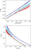 |
Fig. 6 Surface abundance of [C/N] for clump stars as a function of stellar ages (top panel) and stellar masses (bottom panel) for a synthetic thin disc computed with the BGM. Stars are divided in three metallicity-bins: −0.20 ≤ [Fe/H] ≤−0.10 (blue dots), −0.05 ≤ [Fe/H] ≤ +0.05 (green dots), and +0.15 ≤ [Fe/H] ≤ +0.25 (red dots). Relations between [C/N] and mass and age (Eqs. (3) and (4)) are also shown with the solid lines. |
In this context, Fig. 5 (coloured-dots) shows the impact of thermohaline instability on the [C/N] versus age and versus mass diagrams. As thermohaline instability changes the surface abundances in carbon and nitrogen after the bump, large dispersions of [C/N] with mass and age are noticeable for upper-RGB stars. Since this mechanism does not significantly affect the surface chemical properties of clump stars, relationships between [C/N] with masses and ages can be established. These relationships can be determined at a given metallicity for clump stars contrary to upper-RGB stars.
Figure 6 shows thin-disc clump stars divided in three [Fe/H]-bins: (1) lower metallicity (−0.20 ≤ [Fe/H] ≤−0.10); (2) solar metallicity (−0.05 ≤ [Fe/H] ≤ +0.05); (3) higher metallicity (+0.15 ≤ [Fe/H] ≤ +0.25). In Eqs. (3) and (4), we present relations allowing for the estimation of the stellar masses and ages (resp.) of clump stars from [C/N] abundance ratio, in each metallicity range, assuming the stellar physics described above and taking into account the effects of thermohaline mixing. ![Mathematical equation: \begin{eqnarray} M/M_{\odot} = \left \{ \begin{aligned} 15.66\cdot[{\rm C/N}]^{2}+11.27\cdot[{\rm C/N}]+2.887 \\ \qquad \text{for} -0.20 \leq [{\rm Fe/H}] \leq -0.10\\ 13.94\cdot[{\rm C/N}]^{2}+9.554\cdot[{\rm C/N}]+2.603\\ \qquad \text{for} -0.05 \leq [{\rm Fe/H}] \leq +0.05\\ 17.71\cdot[{\rm C/N}]^{2}+12.49\cdot[{\rm C/N}]+3.313\\ \qquad \text{for} +0.15 \leq [{\rm Fe/H}] \leq +0.25 \end{aligned} \right. \label{rel_mass} \end{eqnarray}](/articles/aa/full_html/2017/05/aa30253-16/aa30253-16-eq40.png) (3)
(3)![Mathematical equation: \begin{eqnarray} \log ({\rm Age[yr]}) = \left \{ \begin{aligned} 1.932\cdot[{\rm C/N}]^{2}+7.904\cdot[{\rm C/N}]+13.27 \\ \qquad \text{for} -0.20 \leq [{\rm Fe/H}] \leq -0.10\\ 1.317\cdot[{\rm C/N}]^{2}+6.329\cdot[{\rm C/N}]+12.50 \\ \qquad \text{for} -0.05 \leq [{\rm Fe/H}] \leq +0.05\\ -2.766\cdot[{\rm C/N}]^{2}+1.845\cdot[{\rm C/N}]+11.13 \\ \qquad \text{for} +0.15 \leq [{\rm Fe/H}] \leq +0.25. \end{aligned} \right. \label{rel_age} \end{eqnarray}](/articles/aa/full_html/2017/05/aa30253-16/aa30253-16-eq41.png) (4)Importantly, the relation with age depends on the stellar model used. It is then crucial to validate the models and the mixing processes before using ages for Galactic archeology. In a forthcoming paper, we shall discuss the effects of rotation on these relations and estimate the accuracy of age and mass determinations using surface chemical properties.
(4)Importantly, the relation with age depends on the stellar model used. It is then crucial to validate the models and the mixing processes before using ages for Galactic archeology. In a forthcoming paper, we shall discuss the effects of rotation on these relations and estimate the accuracy of age and mass determinations using surface chemical properties.
6. Conclusions
In this paper, we have presented a new version of the Besançon stellar population synthesis model of the Galaxy, including a new grid of stellar evolution models computed with the code STAREVOL. This new stellar grid of single-star evolution models is computed for five metallicities in the mass range between 0.6 and 6.0 M⊙, including the effects of thermohaline instability during the red-giant branch. These models provide the global (e.g. surface gravity, effective temperature), chemical (surface properties for 54 stable and unstable species), and seismic properties (Δν, νmax, ΔΠ(ℓ = 1)). Thermohaline mixing occurring in thin disc giants has been shown to produce measurable effects on the chemical properties, in particular on 12C/13C and [C/N] ratios. Stellar evolution models at different α-enhancement are being computed to study the older populations, such as the thick disc, the halo, and the bulge, and will be presented in a forthcoming paper.
By comparing the BGM simulations with observations from large spectroscopic and seismic surveys, we are able to constrain the physics of the transport processes occurring in stellar interiors. Red giants observed from asteroseismology can be now used as new cosmic clocks, allowing age calibration from chemical observations. Applying the new version of the BGM, we derive mean relations between [C/N] and age, usable to estimate ages for thin-disc red-clump giants, when their metallicity is known. Contrarily to previously derived relationships, ours take into account the natural spread in mass and metallicity of the underlying population, and allows for the inclusion of selection biases in the surveys. In a forthcoming paper of this series, we shall investigate the impact of different prescriptions for thermohaline instability on these relations, as well as the effect of rotation-induced mixing.
Thanks to WEAVE, 4MOST, and PLATO, the future looks extremely promising in terms of collecting spectroscopic and seismic data for a large number of stars. The Besançon Galaxy model will be a key tool to prepare these future instruments and missions as well as to exploit a large amount of data from Gaia, giving a better understanding of stellar and Galactic evolution.
Acknowledgments
We acknowledge financial support from “Programme National de Physique Stellaire” (PNPS) of CNRS/INSU, France. N.L. acknowledges financial support from the CNES fellowship.
References
- Ackerstaff, K., Airapetian, A., Akopov, N., et al. 1998, Nucl. Inst. Meth. Phys. Res. A, 417, 230 [Google Scholar]
- Anders, F., Chiappini, C., Rodrigues, T. S., et al. 2016, Astron. Nachr., 337, 926 [NASA ADS] [CrossRef] [Google Scholar]
- Angelou, G. C., Church, R. P., Stancliffe, R. J., Lattanzio, J. C., & Smith, G. H. 2011, ApJ, 728, 79 [NASA ADS] [CrossRef] [Google Scholar]
- Angelou, G. C., Stancliffe, R. J., Church, R. P., Lattanzio, J. C., & Smith, G. H. 2012, ApJ, 749, 128 [NASA ADS] [CrossRef] [Google Scholar]
- Asplund, M., Grevesse, N., Sauval, A. J., & Scott, P. 2009, ARA&A, 47, 481 [NASA ADS] [CrossRef] [Google Scholar]
- Baglin, A., & Fridlund, M. 2006, in The CoRoT Mission Pre-Launch Status, Stellar Seismology and Planet Finding, eds. M. Fridlund, A. Baglin, J. Lochard, & L. Conroy, ESA SP, 1306, 11 [Google Scholar]
- Beck, P. G., Montalban, J., Kallinger, T., et al. 2012, Nature, 481, 55 [NASA ADS] [CrossRef] [Google Scholar]
- Bedding, T. R., Mosser, B., Huber, D., et al. 2011, Nature, 471, 608 [NASA ADS] [CrossRef] [PubMed] [Google Scholar]
- Belkacem, K., Goupil, M. J., Dupret, M. A., et al. 2011, A&A, 530, A142 [NASA ADS] [CrossRef] [EDP Sciences] [Google Scholar]
- Bossini, D., Miglio, A., Salaris, M., et al. 2015, MNRAS, 453, 2290 [NASA ADS] [CrossRef] [Google Scholar]
- Chabrier, G., & Baraffe, I. 1997, A&A, 327, 1039 [NASA ADS] [Google Scholar]
- Charbonnel, C. 1994, A&A, 282, 811 [NASA ADS] [Google Scholar]
- Charbonnel, C., & Lagarde, N. 2010, A&A, 522, A10 [NASA ADS] [CrossRef] [EDP Sciences] [MathSciNet] [PubMed] [Google Scholar]
- Charbonnel, C., & Zahn, J.-P. 2007, A&A, 467, L15 [NASA ADS] [CrossRef] [EDP Sciences] [Google Scholar]
- Charbonnel, C., Brown, J. A., & Wallerstein, G. 1998, A&A, 332, 204 [NASA ADS] [Google Scholar]
- Cui, X.-Q., Zhao, Y.-H., Chu, Y.-Q., et al. 2012, Res. Astron. Astrophys., 12, 1197 [NASA ADS] [CrossRef] [Google Scholar]
- Czekaj, M. A., Robin, A. C., Figueras, F., Luri, X., & Haywood, M. 2014, A&A, 564, A102 [NASA ADS] [CrossRef] [EDP Sciences] [Google Scholar]
- Denissenkov, P. A. 2010, ApJ, 723, 563 [NASA ADS] [CrossRef] [Google Scholar]
- Drazdauskas, A., Tautvaišienė, G., Randich, S., et al. 2016, A&A, 589, A50 [NASA ADS] [CrossRef] [EDP Sciences] [Google Scholar]
- Eggleton, P. P., Dearborn, D. S. P., & Lattanzio, J. C. 2006, Science, 314, 1580 [NASA ADS] [CrossRef] [PubMed] [Google Scholar]
- Eggleton, P. P., Dearborn, D. S. P., & Lattanzio, J. C. 2008, ApJ, 677, 581 [NASA ADS] [CrossRef] [Google Scholar]
- Freeman, K., & Bland-Hawthorn, J. 2002, ARA&A, 40, 487 [NASA ADS] [CrossRef] [Google Scholar]
- Fusi Pecci, F., Ferraro, F. R., Crocker, D. A., Rood, R. T., & Buonanno, R. 1990, A&A, 238, 95 [NASA ADS] [Google Scholar]
- Gaia Collaboration (Brown, A. G. A., et al.) 2016, A&A, 595, A2 [NASA ADS] [CrossRef] [EDP Sciences] [Google Scholar]
- Gilliland, R. L., Brown, T. M., Christensen-Dalsgaard, J., et al. 2010, PASP, 122, 131 [NASA ADS] [CrossRef] [Google Scholar]
- Gilmore, G., Randich, S., Asplund, M., et al. 2012, The Messenger, 147, 25 [NASA ADS] [Google Scholar]
- Haywood, M. 2008, MNRAS, 388, 1175 [NASA ADS] [CrossRef] [Google Scholar]
- Krishnamurti, R. 2003, J. Fluid Mech., 483, 287 [NASA ADS] [CrossRef] [Google Scholar]
- Lagarde, N., Charbonnel, C., Decressin, T., & Hagelberg, J. 2011, A&A, 536, A28 [NASA ADS] [CrossRef] [EDP Sciences] [Google Scholar]
- Lagarde, N., Decressin, T., Charbonnel, C., et al. 2012a, A&A, 543, A108 [NASA ADS] [CrossRef] [EDP Sciences] [Google Scholar]
- Lagarde, N., Romano, D., Charbonnel, C., et al. 2012b, A&A, 542, A62 [NASA ADS] [CrossRef] [EDP Sciences] [Google Scholar]
- Lagarde, N., Miglio, A., Eggenberger, P., et al. 2015, A&A, 580, A141 [NASA ADS] [CrossRef] [EDP Sciences] [Google Scholar]
- Lagarde, N., Bossini, D., Miglio, A., Vrard, M., & Mosser, B. 2016, MNRAS, 457, L59 [NASA ADS] [CrossRef] [Google Scholar]
- Lebreton, Y., Goupil, M. J., & Montalbán, J. 2014a, in EAS Pub. Ser., 65, 99 [Google Scholar]
- Lebreton, Y., Goupil, M. J., & Montalbán, J. 2014b, in EAS Pub. Ser., 65, 177 [Google Scholar]
- Majewski, S. R., Schiavon, R. P., Frinchaboy, P. M., et al. 2015, AJ, submitted [arXiv:1509.05420] [Google Scholar]
- Marshall, D. J., Robin, A. C., Reylé, C., Schultheis, M., & Picaud, S. 2006, A&A, 453, 635 [NASA ADS] [CrossRef] [EDP Sciences] [Google Scholar]
- Martig, M., Rix, H.-W., Aguirre, V. S., et al. 2015, MNRAS, 451, 2230 [NASA ADS] [CrossRef] [Google Scholar]
- Masseron, T., & Gilmore, G. 2015, MNRAS, 453, 1855 [NASA ADS] [CrossRef] [Google Scholar]
- Masseron, T., Lagarde, N., Miglio, A., Elsworth, Y., & Gilmore, G. 2017, MNRAS, 464, 3021 [NASA ADS] [CrossRef] [Google Scholar]
- Miglio, A. 2012, in Asteroseismology of Red Giants as a Tool for Studying Stellar Populations: First Steps, eds. A. Miglio, J. Montalbán, & A. Noels (Heidelberg: Springer-Verlag), 11 [Google Scholar]
- Miglio, A., Montalbán, J., Carrier, F., et al. 2010, A&A, 520, L6 [NASA ADS] [CrossRef] [EDP Sciences] [Google Scholar]
- Miglio, A., Chiappini, C., Morel, T., et al. 2013, MNRAS, 429, 423 [NASA ADS] [CrossRef] [Google Scholar]
- Mikolaitis, Š., Tautvaišienė, G., Gratton, R., Bragaglia, A., & Carretta, E. 2010, MNRAS, 407, 1866 [NASA ADS] [CrossRef] [Google Scholar]
- Morel, T., Miglio, A., Lagarde, N., et al. 2014, A&A, 564, A119 [NASA ADS] [CrossRef] [EDP Sciences] [Google Scholar]
- Mosser, B., Belkacem, K., Goupil, M.-J., et al. 2010, A&A, 517, A22 [NASA ADS] [CrossRef] [EDP Sciences] [Google Scholar]
- Mosser, B., Goupil, M. J., Belkacem, K., et al. 2012a, A&A, 548, A10 [NASA ADS] [CrossRef] [EDP Sciences] [Google Scholar]
- Mosser, B., Goupil, M. J., Belkacem, K., et al. 2012b, A&A, 540, A143 [NASA ADS] [CrossRef] [EDP Sciences] [Google Scholar]
- Mosser, B., Michel, E., Belkacem, K., et al. 2013, A&A, 550, A126 [NASA ADS] [CrossRef] [EDP Sciences] [Google Scholar]
- Palacios, A., Charbonnel, C., Talon, S., & Siess, L. 2006, A&A, 453, 261 [NASA ADS] [CrossRef] [EDP Sciences] [Google Scholar]
- Robin, A. C., Reylé, C., Derrière, S., & Picaud, S. 2003, A&A, 409, 523 [NASA ADS] [CrossRef] [EDP Sciences] [Google Scholar]
- Robin, A. C., Marshall, D. J., Schultheis, M., & Reylé, C. 2012, A&A, 538, A106 [NASA ADS] [CrossRef] [EDP Sciences] [Google Scholar]
- Robin, A. C., Reylé, C., Fliri, J., et al. 2014, A&A, 569, A13 [NASA ADS] [CrossRef] [EDP Sciences] [Google Scholar]
- SDSS Collaboration (Albareti, F. D., et al.) 2016, ApJS, submitted [arXiv:1608.02013] [Google Scholar]
- Smiljanic, R., Gauderon, R., North, P., et al. 2009, A&A, 502, 267 [NASA ADS] [CrossRef] [EDP Sciences] [Google Scholar]
- Steinmetz, M., Zwitter, T., Siebert, A., et al. 2006, AJ, 132, 1645 [NASA ADS] [CrossRef] [Google Scholar]
- Stello, D., Bruntt, H., Preston, H., & Buzasi, D. 2008, ApJ, 674, L53 [NASA ADS] [CrossRef] [Google Scholar]
- Tassoul, M. 1980, ApJS, 43, 469 [NASA ADS] [CrossRef] [Google Scholar]
- Tautvaišienė, G., Barisevičius, G., Chorniy, Y., Ilyin, I., & Puzeras, E. 2013, MNRAS, 430, 621 [NASA ADS] [CrossRef] [Google Scholar]
- Tautvaišienė, G., Drazdauskas, A., Mikolaitis, Š., et al. 2015, A&A, 573, A55 [NASA ADS] [CrossRef] [EDP Sciences] [Google Scholar]
- Tautvaišienė, G., Drazdauskas, A., Bragaglia, A., Randich, S., & Ženovienė, R. 2016, A&A, 595, A16 [NASA ADS] [CrossRef] [EDP Sciences] [Google Scholar]
- Traxler, A., Garaud, P., & Stellmach, S. 2011, ApJ, 728, L29+ [NASA ADS] [CrossRef] [Google Scholar]
- Turon, C., Primas, F., Binney, J., et al. 2008, The Messenger, 134, 46 [Google Scholar]
- Ulrich, R. K. 1972, ApJ, 172, 165 [NASA ADS] [CrossRef] [Google Scholar]
- Vrard, M., Mosser, B., & Samadi, R. 2016, A&A, 588, A87 [NASA ADS] [CrossRef] [EDP Sciences] [Google Scholar]
- Yanny, B., Rockosi, C., Newberg, H. J., et al. 2009, AJ, 137, 4377 [NASA ADS] [CrossRef] [Google Scholar]
All Tables
All Figures
|
Fig. 1 Theoretical evolution of 3He and carbon isotopic ratio at the stellar surface as a function of surface gravity for stellar models of: left panels various masses (1.0; 1.2; 1.5; 1.8; 3.0 M⊙ represented by a black, red, blue, green and orange solid line, respectively) at Z = 0.04; right panels various metallicities ([Fe/H] = 0.5; 0; −0.23; −0.54; −2.14 represented by a black, red, blue, green and orange solid line, respectively) at M = 1.2 M⊙. These models include the effects of thermohaline instability (bottom panels) and following standard evolution (top panels). These tracks are shown from the main sequence up to the early-AGB. |
| In the text | |
|
Fig. 2 Large separation, Δν, as a function of the effective temperature, Teff, for synthetic population computed with the BGM. Colours indicate the νmax, the frequency at which the power spectrum is maximum. |
| In the text | |
|
Fig. 3 Surface gravity as a function of effective temperature for synthetic populations computed with the BGM including the effects of thermohaline instability (right panel) or not (left panel). The colour code represents the carbon isotopic ratio at the surface of stars in the thin disc. |
| In the text | |
|
Fig. 4 Surface abundance of 3He (in mass fraction, top-left panel), 12C/13C (top-right panel), [C/Fe] (bottom-left panel), and [N/Fe] (bottom-right panel) as a function of stellar mass for synthetic thin disc computed with the BGM. Stars have been selected to be in the clump according to their ΔΠℓ = 1. The colour code represents the metallicity of stars. Simulations including or not the effects of thermohaline instability are represented by colour-dots and crosses respectively. |
| In the text | |
|
Fig. 5 Surface abundance of [C/N] as a function of stellar ages (left panels) and stellar masses (right panels), colour-coded by metallicity, for a synthetic thin disc computed with the BGM. Stars have been selected to be in the clump according to their ΔΠℓ = 1, as well as before and after the RGB-bump according to their log(g) values. Simulations including or not the effect of thermohaline instability are shown as colour-dots and grey crosses respectively. |
| In the text | |
|
Fig. 6 Surface abundance of [C/N] for clump stars as a function of stellar ages (top panel) and stellar masses (bottom panel) for a synthetic thin disc computed with the BGM. Stars are divided in three metallicity-bins: −0.20 ≤ [Fe/H] ≤−0.10 (blue dots), −0.05 ≤ [Fe/H] ≤ +0.05 (green dots), and +0.15 ≤ [Fe/H] ≤ +0.25 (red dots). Relations between [C/N] and mass and age (Eqs. (3) and (4)) are also shown with the solid lines. |
| In the text | |
Current usage metrics show cumulative count of Article Views (full-text article views including HTML views, PDF and ePub downloads, according to the available data) and Abstracts Views on Vision4Press platform.
Data correspond to usage on the plateform after 2015. The current usage metrics is available 48-96 hours after online publication and is updated daily on week days.
Initial download of the metrics may take a while.