| Issue |
A&A
Volume 600, April 2017
|
|
|---|---|---|
| Article Number | A134 | |
| Number of page(s) | 14 | |
| Section | Astrophysical processes | |
| DOI | https://doi.org/10.1051/0004-6361/201629796 | |
| Published online | 13 April 2017 | |
Shock-cloud interaction and gas-dust spatial separation
Centre for mathematical Plasma Astrophysics, Department of Mathematics, KU Leuven Celestijnenlaan 200B, 3001 Leuven, Belgium
e-mail: This email address is being protected from spambots. You need JavaScript enabled to view it.
Received: 27 September 2016
Accepted: 13 January 2017
Abstract
Context. We revisit the study of shocks interacting with molecular clouds, incorporating coupled gas-dust dynamics.
Aims. We study the effect of different parameters on the shock-cloud interaction, such as the dust-to-gas ratio or the Mach number of the impinging shock. By solving self-consistently for drag-coupled gas and dust evolutions, we can assess the frequently made assumption that the dust is locked to the dynamics of the gas so that dust observations would result in direct information on the gas distribution.
Methods. We used a multi-fluid model where the dust is represented by grain-size specific pressureless fluids. The dust and gas interact through a drag force, and we used four dust species with weighted representative sizes between 1 and 500 nm. We use the open source code MPI-AMRVAC for a parametric study of the effect of the gas-dust ratio and the Mach number of the shock. By using the radiative transfer code SKIRT, we create synthetic millimeter wavelength maps to connect to observations.
Results. We find that the presence of dust does not significantly affect the dynamics of the gas for realistic dust-gas ratios, and this is the case throughout the range of Mach numbers explored (1.5−10). For high Mach numbers, we find a significant discrepancy between the distribution of the dust and gas after the cloud-shock interaction with the larger dust species clearly lagging the heavily mixed and accelerated gas (re)distribution.
Conclusions. We conclude that observational studies of dusty environments may need to account for clearly separated spatial distributions of dust and gas, especially those studies that are representative of molecular clouds that have been interacting with high Mach number shock fronts.
Key words: ISM: clouds / dust, extinction / hydrodynamics
© ESO, 2017
1. Introduction
Matter in the dilute interstellar medium (ISM) is mostly atomic (HI) and molecular (H2) hydrogen gas, but their precise amounts can be difficult to quantify. Observers resort to HI 21 cm emission, or CO rotational emission lines, to indirectly trace the total gas content. Another important tracer is dust, which plays a fundamental role in the observations: dust reprocesses a significant percentage of the stellar light, either by scattering (and polarizing) it or by absorbing it, causing wavelength dependent interstellar extinction. The resulting warmer dust then emits in the infrared. Inferred dust temperatures remain low, for example in between 20 to 30 K in two well-diagnosed molecular clouds in the LMC known as NT80 and NT71 (Roman-Duval et al. 2010). Dust in dense clouds can shield H2 and its tracer CO from radiative dissociation. As a result of all these effects, knowing the spatial distribution of the dust and its optical properties (extinction/emission coefficient) is crucial to all observations.
The dust mass content is rather low, i.e. of order 1 percent of the gas content, as for example inferred by Lilley (1955) for dust clouds in Taurus, Orion, and Perseus. Lilley (1955) used HI 21 cm emission in a region about the galactic anticentre to demonstrate a clear correlation (in latitude and longitude) between gas and dust distributions; for example, brightness variation in the radio emission and optical extinction derived from galaxy counts are found to be well correlated.
Using high resolution Herschel observations, Roman-Duval et al. (2010) critically assessed the dust-gas correlation in view of the excess far-infrared emission near molecular clouds when compared to gas surface densities traced by CO or HI 21 cm. Their study quantifies the ratio of gas surface densities implied from dust versus those inferred from CO and HI observations for NT80 and NT71, as showing variation between [0.2−2.8]. They conclude that there is a spatial correlation between dust and atomic to molecular gas phases and that explaining the far-infrared excess regions may not call for significant gas-to-dust ratio variations. Indeed, they assume a constant value (351 for NT80 and 234 for NT71) when deducing the gas content from the dust.
Although the dust-to-gas correlation in molecular clouds is thus well accepted at large scales (giant molecular clouds), the possibility exists that significant variation in the gas to dust distributions is important at smaller scales, such as in isolated bok globules. We address this here with numerical simulations, benefitting from efforts that have been made in recent years to model the interaction between the dust grains and the gas. A fair variety of numerical algorithmic approaches have been adopted, such as fully particle-based two-fluid smoothed-particle hydrodynamics (SPH) methods (Cha & Nayakshin 2011; Laibe & Price 2012) to hybrid particle-fluid methods (Johansen et al. 2006; Miniati 2010) and two-fluid hydrodynamic models (Paardekooper & Mellema 2006; van Marle et al. 2011; Meheut et al. 2012).
A first result of these studies is that we have started to realize that local spatial discrepancy between gas and dust accumulations can become significant in turbulent gases or can naturally arise from developing instabilities. In Hopkins & Lee (2016), a study of how grains behave in supersonic turbulence in magnetized molecular clouds, under isothermal assumptions, and with subdominant Lorentz forces, these investigators demonstrated the formation of filamentary structure in the dust with gas and dust filaments found in spatially different locations. Hendrix & Keppens (2014) focussed on local box shear flow evolutions and found that dust grains of different sizes are partly-to-fully evacuated from vortex cores that result from Kelvin-Helmholtz instabilities; these dust grains also form clear filamentary distributions, which can explain the power-law tails in the log-normal column density distributions without invoking self-gravity. Both studies have found that their local dust-to-gas ratio can change by several orders of magnitude. In protoplanetary disks, this dissociation is essential to enable the formation of larger structure (for ultimate planetesimal formation) and can arise from Rossby wave instabilities in accretion disks (Meheut et al. 2012). In van Marle et al. (2011), a wind-ISM collision set-up demonstrated that the larger grain populations especially may show deviations from gas morphology and penetrate even beyond the overarching bow shock.
These simulations all emphasize relatively small spatial separations, for example internal to larger structures such as molecular clouds. The question arises whether such separation could be large enough to be observed and resolved by modern instruments. For this reason, we investigate what happens when a strong shock interacts with an isolated molecular cloud and whether we can achieve a separation on the scale of the size of the object itself. The study of hydrodynamic shock-cloud interaction has been studied by many authors, and Pittard et al. (2009) gives a good review of studies made on this interaction. Different physical processes have already been considered in detail, such as radiative cooling or thermal conduction or extending hydro simulations to magnetohydrodynamic regimes. Since the hydro set-ups have not yet taken the presence of dust into account, we study this in a regime that is relevant for small molecular clouds, and look at the dynamical effect of the dust on the destruction of a molecular cloud by a shock.
2. Simulation set-up
We use the MPI-AMRVAC code (Keppens et al. 2012; Porth et al. 2014) to simulate the interaction between the shock and the molecular cloud (MC). The inclusion of dust in the code is discussed in van Marle et al. (2011) and several tests are reported in Porth et al. (2014). All our simulations use the same model: a multi-fluids dust-hydro simulation in which four species of dust are incorporated as pressureless fluids. The interaction between the gas density and dust populations is through an interaction term fd entering the momentum and energy equations (Eqs. (3),(4)) of the hydrodynamic Euler set as a source term. This term is for each dust species given by 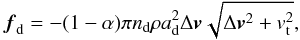 (1)where d ∈ (1:4) is the index of the dust species; (1−α) is a measure of the effectiveness of momentum transfer from gas to dust and vice versa, where α = 0.25 is a good choice according to Kwok (1975); nd is the dust particle density; ad is the grain radius; Δv is the difference between the gas and dust velocities (Δv = v−vd); and
  (Kwok 1975) is the thermal speed of the gas, where p and ρ are the pressure and density of the gas.
The hydrodynamic equations for the gas is written as ![Mathematical equation: \begin{eqnarray} && \frac{\partial \rho}{\partial t} + \bigtriangledown \cdot (\rho \vec{v})=0, \label{matter} \\ && \frac{\partial (\rho \vec{v})}{\partial t} + \bigtriangledown \cdot (\rho \vec{v} \vec{v}) + \bigtriangledown p= \sum\limits_{d=1}^4 \vec{f}_{\rm d}, \label{momentum} \\ && \frac{\partial e}{\partial t}+\bigtriangledown \cdot [(p+e)\vec{v}] = \sum\limits_{d=1}^4 \vec{v} \cdot \vec{f}_{\rm d}, \label{energy} \\ && e=\frac{p}{\gamma-1}+\frac{\rho v^2}{2}, \end{eqnarray}](/articles/aa/full_html/2017/04/aa29796-16/aa29796-16-eq17.png) where e is the total energy density of the gas, γ the polytropic index of the gas equal to 5/3, and fd the drag force as defined before. The equations for the dust as pressureless fluids are
where e is the total energy density of the gas, γ the polytropic index of the gas equal to 5/3, and fd the drag force as defined before. The equations for the dust as pressureless fluids are
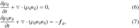 where ρd is the dust density. The model is described in more detail in Hendrix & Keppens (2014). We do not have any creation or destruction of dust in contrast to Hendrix et al. (2016), in which dust redistribution in a binary stellar system due to wind-wind collision was studied and in which gas-to-dust formation was parametrically treated.
As shown in Porth et al. (2014; Fig. 3 of their paper), it is possible to avoid spatial dephasing in linear sound (gas-dust) wave propagation without imposing an extra stopping-time related spatial resolution criterion, if one adopts higher order schemes. Using a TVDLF scheme with an MC or Woodward limiter does suffer from dephasing, but stays limited to a few percent at least for the idealized dusty wave test from Laibe & Price (2012). For the time step constraint, we actually combine a standard CFL criterion with the drag stopping time criterion from Laibe & Price (2012).
We use an idealized typical shock-cloud configuration with a simple spherical molecular cloud represented as an overdensity of the gas. This setup is mainly characterized by the density ratio of the cloud core to the ISM density χ = ρcloud/ρISM and by its radius rc. We use a profile similar to Pittard et al. (2009) and Nakamura et al. (2006). The radial density profile internal to the cloud is ![Mathematical equation: \begin{equation} \rho(r)=\rho_{\rm ISM}[\psi+(1-\psi)\eta_{\rm c}], \end{equation}](/articles/aa/full_html/2017/04/aa29796-16/aa29796-16-eq26.png) (8)where
(8)where ![Mathematical equation: \begin{equation} \eta_{\rm c}=\frac{1}{2}\left [1+\frac{\alpha_{\rm c}-1}{\alpha_{\rm c}+1}\right], \end{equation}](/articles/aa/full_html/2017/04/aa29796-16/aa29796-16-eq27.png) (9)with αc = exp { min [20.0,p1((r/rc)2−1)] }. The constant ψ is adjusted to obtain the specified density contrast χ for the centre of the cloud. The parameter p1 controls the steepness of this profile. For p1 ≳ 5, we find ψ ≈ χ. We use p1 = 10 to obtain a profile that is similar to Pittard et al. (2009), which allows for direct comparison.
(9)with αc = exp { min [20.0,p1((r/rc)2−1)] }. The constant ψ is adjusted to obtain the specified density contrast χ for the centre of the cloud. The parameter p1 controls the steepness of this profile. For p1 ≳ 5, we find ψ ≈ χ. We use p1 = 10 to obtain a profile that is similar to Pittard et al. (2009), which allows for direct comparison.
In the initial conditions, the dust is only present in the molecular cloud. Its total density over the different populations is taken to be equal to a set ratio with the gas density in the cloud η = ρdust/ρcloud. We make the assumption that the dust are silicate grains resulting in an internal grain density of ρp = 3.3 g cm-3 (Draine & Lee 1984). The dust grains follow a size distribution between 1 nm and 500 nm with a slope ∝ r-3.5. This population is then cut into four bins. We label these dust species as d1, d2, d3, and d4 with representative sizes of 1.66 × 10⁻³, 5.9 × 10⁻², 0.18, and 0.36μm.
We use seven levels of refinement for our AMR scheme. In all cases, rc is taken equal to the unit of length, which we set to 1 parsec. This results in a minimal effective resolution of 64 cells per cloud radius rc. We ensure the resolution (by forcing AMR) to be maximal around the cloud core to be able to accurately follow the interaction with the shock. Two-dimensional set-ups use an (R,Z) domain with symmetry about the R = 0 axis. The domain uses 24 units of length (= 24rc) in the radial direction. This ensures that no material from the cloud may leave through the radial boundary during the times covered. In the Z direction, the domain is chosen to be long enough so the material from the cloud cannot reach the end of the simulation box. This may vary with the different simulations.
The shock front is defined as a step function that travels from negative to positive Z. The conditions behind the shock front are calculated from Rankine-Hugoniot conditions, which depend on the Mach number of the shock defined as M = us/cs, where us is the shock travelling speed and cs the sound speed in the region in front of the shock. The density ratio and velocity ratio before and after the shock can be expressed as 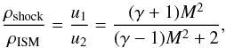 (10)where u1 and u2 are the gas velocity before and after the shock in the shock frame. In the observer frame, this translates to u1 = −us and u2 = vshock−us, where vshock is the velocity of the gas in the shocked region. The pressure ratio before and after the shock can be expressed as
 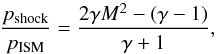 (11)where pshock is the pressure in the shocked region and pISM the pressure in the ISM.
As discussed in Pittard et al. (2009), the destruction of a MC by a shock is essentially scale free and depends only on the Mach number M of the shock and the density ratio χ between the cloud core and the medium. The code runs with adimensional code units. To relate our results to galactic molecular clouds, we report results in physical units following the normalization we adopted as follows: a unit of length is 1 pc = 3.0857 × 1018cm, a unit of density with one proton per cm3 or 1.6726 × 10⁻²⁴ g cm-3 and a fiducial speed value of 1 × 108 cm s-1, setting the code unit of time as 978.34 yr. The post-shock is initialized on a 1 pc band at the bottom of the domain and the cloud is located at 5 pc on the Z-axis.
The ISM is taken to be a hot ISM with temperature 105 K and a density of 1 proton per cm3. As our cloud is in pressure equilibrium with the ISM, a density ratio χ = 1000 results in a temperature equal to 100 K for the cloud. These parameters are chosen as a good representation for a part of our galaxy close to dense stellar activity where shocks are more likely to be encountered (see Ferrière 2001).
Looking at the cooling curve for the ISM, 105 K is actually at the peak for (optically thin) radiative loss. Taking values for the cooling rate from Schure et al. (2009), we find the cooling timescale for this temperature to be  (12)with kb the Boltzman constant, Λ(T) the cooling rate, and nH the number density of proton with mean molecular weight μ. For our temperature of 105 K we find tcool of the order of a kyr, which is much shorter than our simulation timescale. Ferrière (2001) gives an explanation that radiative cooling in these regions are in fact in equilibrium with heating from photoionization resulting from nearby stellar activity, which is why we adopt here a constant 105 K hot ISM condition. Furthermore, the denser, colder conditions in our clouds are at least initially not subject to cooling. For this reason, we use a purely adiabatic simulation and leave a more realistic treatment of radiative effects, such as photoionization and the possible creation of thin shocked cloud shells due to radiative cooling, for future work.
Parameters for the various simulations.
With this set-up, we run various cases and a summary of the geometry and parameters used in each case can be found in Table 1. These include two series of cases allowing for two separated parametric studies. The cases m10noD, and m10loD, m10meD, and m10hiD are meant to study the effect of the presence of dust on the dynamics of the interaction between a MC and a shock by gradually increasing the dust-to-gas ratio. On the other hand, cases m1.5loD, m3loD, and m10loD study the effect of the Mach number of the shock on that interaction. The case m10loDzoom shows a more resolved local view on case m10loD, and is discussed briefly in Sect. 3.3, while m10loD3D is a 3D version of m10loD that is used for synthetic maps in Sect. 3.4. The parameters for all cases can be compared with the results without dust in Pittard et al. (2010).
Timescales deduced from the simulations.
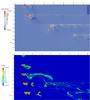 |
Fig. 1 For case m10loD. Top: logarithm of gas density for times 100, 200, 540, and 700 kyr. These times correspond to a first, second, and third interaction peak, and the post-mixing phase. The symmetry axis is horizontal. Bottom: views on the dust-to-gas ratio (DGR) for the same times (and for our initial condition). |
3. Results
Table 2 gives resulting timescales for the simulations, where we quantify how mixing processes alter the cloud properties after the shock impact. By using a passive tracer that identifies where the original cloud material ends up, we find tmix as the time needed for the mass of the cloud core to become reduced by half. The cloud core is defined as the region of the MC in which the tracer has a value higher or equal to 0.8 (with its initial value set to 1 in the entire cloud). We can then compute the mass using this tracer region as a mask. Similarly, ttot is the time for the cloud core mass to be less than 5% of its initial value, and this value would represent almost total destruction of the cloud. The ratio tmix/tcc can be compared to Pittard et al. (2010), where tcc is a cloud crushing normalization time that we describe later on, but in essence allows us to inter-compare various Mach number runs, which evolve on rather different timescales. Three other regions are used in the following sections; the mixing region is loosely defined as where our tracer adopts values in the open set ] 0,0.8 [. The ISM conditions are initially static, uniform, and known, so we can easily locate the original ISM at rest, which is ahead of the shock. If we then exclude the original ISM, cloud, and mixing region from our domain, we find the shocked interstellar medium (SISM) region.
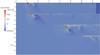 |
Fig. 2 For case m10noD, i.e. the case without dust. Logarithm of the gas density for times equal to 100, 200, 600, and 700 kyr, corresponding to the first, second, and third interaction peak, and post-mixing phase. The symmetry axis is horizontal. |
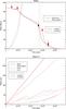 |
Fig. 3 Comparing m10loD with m10noD. Top: evolution of the mass of the cloud core and the mixing region over time. The vertical line corresponds to tmix. The arrows represent the timesteps shown in Figs. 1 and 2. Bottom: evolution of the maximal Z reach of the shocked interstellar medium (SISM) and of the mixing region, together with both maximal and miminal cloud core position. |
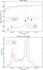 |
Fig. 4 Comparing m10loD with m10noD. Top: mean velocity of the cloud core and in the mixing region. The vertical line corresponds to tmix. The arrows represent the timesteps shown in Figs. 1 and 2. Bottom: kinetic energy evolution of the cloud core. |
3.1. Effect of dust on the dynamics
As already stated, the first parametric set chosen was to quantify the effect of the dust on the dynamics. Figure 1 (top panel) for m10loD (Mach 10 and low dust to gas) and Fig. 2 for m10noD (no dust) show the evolution of the logarithm of the gas density at four representative times, which are selected differently for each case. The first two times correspond to distinct early stages in the shock-cloud interaction as shown later on in Figs. 3,4 when the MC gets accelerated, while the third time is usually nearly coincident with tmix when the mass is reduced by half, and the final time is representative of when the mixing is almost complete (near ttot, or near the endtime simulated). Here the main mechanism of mixing is directly evident; instabilities develop all around the impacted cloud and gradually enlarge the region where material from the cloud mixes with the surroundings. On the bottom panel we can see the dust-to-gas ratio (DGR) for the same four times and for the initial condition, where it simply attains DGR = 4η as it sums over the four dust species. We can clearly see a qualitative difference in the DGR appearance with the gas density. We observe a clear effect of the binning of the dust population with a clear separation of the four species with the bigger dust species showing a retarded rightward evolution. The parameters (shock strength, dust size range, and density contrast) are such that we witness a marked dependence on the grain sizes in their spatial separation from the impacted cloud. We deliberately opted to plot the DGR ratio for all cases, where at the end time, the heavier (d4) to lighter (d1) dust species are encountered from left to right in our plots. The binning gives a clear separation between the four dust species and this DGR variation can be compared to that found in the work of Hopkins & Lee (2016). This DGR parameter is frequently used in observational works and the comparison between the dust species is provided by further figures in the rest of this work.
The four panels of Figs. 3 and 4 especially monitor the evolution of the mass of the MC core, the reach in the Z direction for the different regions as defined in Sect. 3, the mean velocity of the cloud core, and the kinetic energy of the cloud core for both m10loD and m10noD. The arrows indicate the times represented in Figs. 1 and 2, and these figures show how the times correlate with acceleration phases of the cloud core or distinct extrema reached in the cloud core kinetic energy. The mass evolution and velocity evolution can be compared to analogue plots in Pittard et al. (2010) and shows the clear loss of cloud core matter, which is sped up in multiple steps. The rapid evolution of the mixing region mass content in the first panel of Fig. 3 can be explained by the fact that effective mixing causes small quantities of cloud material to be spread over increasingly large volumes of the mixing region mask with corresponding total mass contents beyond the original cloud mass.
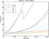 |
Fig. 5 Position of the different dust species and cloud core for m10loD along the Z-axis. |
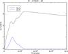 |
Fig. 6 R and Z component of the drag force applied to the d2 dust population. |
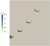 |
Fig. 7 Zoom in for case m10loD, following the blob of dust population d2 for time 310, 470, 630, and 780 kyr. The blob gets deformed and compacted before assuming a wing shape and being stretched in both the R and Z direction. The symmetry axis is vertical. |
We see that destruction of the cloud is a scenario in multiple steps. The first phase is a continuous abrasion from the envelope of the molecular cloud. The mass loss up to this point is small as this strips off the less dense part of the cloud. At the same time the MC starts to be accelerated as seen by the rise in its mean velocity and kinetic energy; see Fig. 4. For both cases m10noD and m10loD, this lasts up to 100 kyr at which point part of the core of the cloud breaks off and starts to be mixed with its surroundings, accompanied by a clear loss of both kinetic energy and mass. The cloud breakdown process really starts when part of the cloud core gets accelerated. This is seen as a clear peak in the mean velocity and kinetic energy of the cloud core. As a result of this acceleration, instabilities develop of generic Kelvin-Helmholtz and Rayleigh-Taylor type from shear flow and relative acceleration. The instabilities cause the accelerated part of the cloud to detach and mix up with the ISM. Pittard et al. (2010) gives the timescale for the KH instabilities to fully develop and cause the cloud to fragment. For the fundamental wavelength this is given as  (13)where tcc is the “cloud crushing time” as defined in Pittard et al. (2009) and corresponding to the time needed by the shock to traverse the radius of the cloud core. This time is written as
  (14)Both tcc and tKH are reported in Table 2. We find tKH of order 102 kyr corresponding to a growth rate of the order 10-2 of the sound speed. This is too short compared to tmix to be the only mechanism of cloud mixing, but this timescale does point out that Kelvin-Helmholtz instabilities are critical to our study. A similar reasoning can be used for Rayleigh-Taylor instability: simple analytic estimates give a growth rate that scales with
  , where our Atwood number A is close to unity due to the large density contrasts; the smallest wavelengths (i.e. largest wave numbers k) should grow faster, although the overall size of the cloud and the shock-cloud gas-dust evolution may preferentially excite modes with wavelengths fitting the size of the cloud. The Rayleigh-Taylor modes show up as the shock acceleration acts as an effective gravity.
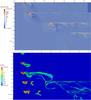 |
Fig. 8 Case m10meD. Top: logarithm of gas density for t equal to 100, 200, 540, and 700 kyr. Bottom: same for the dust-to-gas ratio but with initial conditions. |
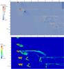 |
Fig. 9 Case m10hiD. Top: logarithm of gas density for t equal to 100, 220, 650, and 700 kyr. Bottom: same for the DGR, with initial conditions. |
The formation of these instabilities has consequences for our tracer-dependent quantification of the cloud core matter. Specifically the Z-reach evolution of the maximal cloud position shows fairly distinct drops at later times; cloud core matter is no longer found further out when a detached cloud fragment mixes to the extent that the accompanying tracer falls below our detection threshold. This also impacts the variation seen in mass evolution, mean velocity, and kinetic energy, but there the computations of mean or total values show much more gradual variations. The maximum Z reach of the mixing region, the region of the domain where there is material from both the cloud and ISM, evolves with a constant velocity. We fit it with a velocity equal to 97% of the gas velocity behind the shock. This is also visible in the plot of the mean velocity where, for the mixing region, it ends up close to the 0.275 × 108 cm s-1 of the post-shock velocity.
When the mixing occurs, it causes a clear change in the mass loss, which is seen as a change in the slope of the mass profile. Our selected times are such that the mass evolution behaves nearly linearly in between them. A first event of this sort happens at 100 kyr for all cases. For m10loD, a second major event takes place at 200 kyr and a third event occurs at 550 kyr, where again we see a rise of the kinetic energy followed by an increased mass loss. The analogue without dust, m10noD, has similar events at 100, 200, and 600 kyr. Again we observe a clear acceleration of the mass loss from phase to phase. Comparing both cases, the presence of a realistic fraction of dust changes only slightly the evolution of the cloud mixing. In both cases we find a tmix of about 550 kyr (see Table 2) and a total mixing time ttot of about 700 kyr.
In Fig. 5 we plot the position of the different dust species and of the cloud core for m10loD. The smaller dust species d1 is mostly linked to the gas dynamics. It follows the cloud core with only minor deviations at a later time. At larger distances it also traces the fragments of the cloud that have been mixed up. On the other hand, the other three species quickly get disconnected: at time 250 kyr, d3 and d4 have completely fallen behind and, at time 300 kyr, d2 has fallen behind. Quite early in the interaction with the shock, the dynamics of the cloud and larger dust species is completely disconnected from direct interaction. This has direct implications for observations as we see in Sect. 3.4.
The general behaviour of the heavier dust is as follows: as these dust species are not linked to the instabilities, they tend to remain in a single blob. Because of the dependence on the gas density of the drag force (see Eq. (1)), the interaction between the gas and dust is especially strong while the dust blob and the cloud are overlapping. A first short period, up to time 10 kyr, has the cloud squeezed towards its centre by the shock. Through the drag force, the same applies to the different dust species, which is seen as a first negative value of its R component (shown in Fig. 6), while its Z component reflects the displacement along the Z-axis. Afterward, from time 10 kyr to 250 kyr the dust blob sees the cloud expanding, but also the flow from the post-shock region being deflected by the overdensity of the cloud. As the dust blob and cloud are still overlapping, this results in a significant R and Z component of the drag force to affect the dust, and a transfer of momentum results. But from the time the disconnection happens at time 250 kyr (see Fig. 5) the dust only sees the flow of the post-shock state whose velocity only has a Z component. Figure 6 shows that the Z component of the drag force (shown here integrated over the area of dust species d2) is steadily decreasing after the disconnection. As the mean density of the dust augments in the blob and the density of the gas is almost constant, this means a diminution of either the volume affected or of the velocity difference Δv. Figure 5 shows that both effects matter as the slope of the reach increases with time and the Z spread decreases. The flattening of the heavier blobs in the Z direction is easily explained as the part of the dust blob facing the incoming flow is more accelerated than the dust blob that is shielded from the incoming flow.
In the R direction, the component of the drag force resulting from the radial component of the incoming flow is small after the overlap phase. We see an increasing spread of the blob in the R direction. This blob, from here on, takes on a wing shape, and we show successive views on it in Fig. 7. This wing is stretched in both R and Z directions by the flow. The point where this happens can clearly be seen in Fig. 5 where the distance between maximum and minimum position starts to increase at time 500 kyr. As the dust is modelled as a pressureless gas, this is purely resulting from interplaying inertial and drag force variations.
As the blob becomes thinner in the Z direction, the difference in acceleration over the blob in the Z direction becomes negligible and the blob is not further compacted. The blob was spherical and is at first compressed in the Z direction. As a result, its mass correspondingly varies in the R direction and is not homogeneously accelerated, resulting in the wing shape already mentioned. The tip of the wing is more easily accelerated resulting in a rapid increase of the total volume occupied by d2, but not of the two drag force components. The reason is that in this volume, Δv quickly tends to zero.
At later times, we see a similar evolution of dust population d3 and d4, and we can assume the same to happen to them but on a timescale that is not yet reached by our simulations.
The follow-up to this first comparison, with and without dust, is to know if dust in higher proportion would significantly change the dynamics. We made two further simulations with a ratio η = ρdust/ρISM equal to 10-2 and 10-1, respectively. An overview of simulation m10meD and m10hiD can be seen in Figs. 8 and 9 giving again a plot of the logarithm of the gas density (top panels) and DGR (bottom panels). For cases m10loD and m10meD, the figures are qualitatively similar in both gas density and DGR, while m10hiD shows more pronounced differences from them in the gas density views. We then make a comparison with the reference m10loD in Figs. 10 and 11. We have the same diagnostics with the four panels that follow the cloud core mass, reach in the Z direction, mean velocity, and kinetic energy.
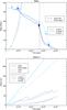 |
Fig. 10 Comparing varying dust ratios. Top: evolution of the mass of the cloud core and mixing region over time. The vertical lines correspond to tmix. The arrows represent the timesteps shown in Figs. 1, 8, and 9. Bottom: evolution of the maximal Z reach of the shocked interstellar medium (SISM), mixing region, maximal cloud core position, and minimal cloud core position. |
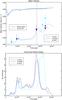 |
Fig. 11 Comparing varying dust ratios. Top: mean velocity of the cloud core and mixing region. The vertical lines correspond to tmix. The arrows represent the timesteps shown in Figs. 1, 8, and 9. Bottom: kinetic energy of the cloud core. |
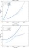 |
Fig. 12 Comparison of the position of the two smaller dust species in m10loD, m10meD, and m10hiD along the Z-axis. Top is species d1 (average 1.66 × 10⁻³μm) and bottom species d2 (average size 5.9 × 10⁻²μm). |
The qualitative behaviour of m10noD, m10loD, m10meD, and m10hiD are very similar. We find again the first event to be around 100 kyr for m10loD, m10meD, and m10hiD. The second event takes place at time 200 kyr for both m10loD and m10meD. For m10hiD this event is retarded by the presence of the dust and happens closer to 250 kyr. We see here a stronger effect of the dust on the dynamics. In particular, we see a stronger effect for m10hiD where we have a density ratio of dust to gas of order 0.1. The third major event takes place for both m10loD and m10meD at time 520 kyr with a clear delay for m10hiD at time 625 kyr. Similarly to m10loD, each event ultimately results in a fraction of the cloud being mixed up and a regression of the reach in the Z direction. Looking at the mass evolution, the delay in the third event for the high dust-loaded case m10hiD also causes a later time tmix for the MC to lose half its mass. But as this event is delayed, we find the material gets accelerated to higher velocity, resulting in more instabilities. This also makes the mixing (and mass loss) stronger than for m10loD and m10meD and results in a higher quantity of material from the MC to be mixed, such that in the end, the total mixing ttot is comparable to the other two cases (see Table 2). This increased turbulence can be seen in Fig. 9 where we also see that the radial spread of the instabilities is increased compared to other cases discussed so far. An interesting fact is that for all cases with strong Mach 10 shocks so far, the period between the second and third major event presents a phase with an almost constant kinetic energy content for the cloud core. Over the same period the mass loss is happening at a fixed rate (i.e. we see a linearly behaving mass evolution curve).
Looking at the two panels of Fig. 12 we follow the evolution of the two smaller dust species, comparing m10loD, m10meD, and m10hiD. Again we find remarkably similar qualitative behaviours despite the drastic difference in dust density. We only see that for lower quantities of dust, it is more easily carried away. In a similar fashion, the higher the dust ratio, the sooner the compression threshold is reached. But even with the large spread of dust density (η values 0.001 to 0.1) the difference is only of a few kyrs, and results in a spatial difference of about 1 parsec. Dust populations d3 and d4 are not reported here as they behave in an almost similar fashion to m10loD both qualitatively and quantitatively. What we can extract from this first parametric study is that it is unlikely for the dust present in molecular clouds to play a critical role in the MC cloud destruction dynamics. This would require dust-to-gas ratios that are far larger than any observations made to date that place this ratio between 0.001 and 0.01. This will most likely play a role in the cloud chemistry and when its charge evolution is followed can become relevant due to magnetic long range forces. However, as we point out in the following, the dust species can separate out far enough to be noticeable in the infrared observations.
3.2. Effect of the Mach number
We observed a significant spatial separation between the heavier dust and gas for an interaction with a strong supersonic shock (M = 10) and a molecular cloud. We now investigate whether such separation would be apparent for an interaction with a less energetic shock. Cases m10loD, m3loD, and m1.5loD evolve on largely different timescales owing to the use of different Mach numbers. To make a comparison between them, we need to scale time with a Mach number dependent constant for each of those three cases. We use for this the “cloud core crushing time” as defined in Eq. (14). We reset the start of normalized time t′ = (t−t0) /tcc to correspond to the moment t0 where the shock first reaches the MC.
Figures 13 and 14 give an overview of the dynamics of m1.5loD and m3loD, this time showing three representative times for gas density and the DGR. As for the previous parametric study, Figs. 15 and 16 give us different diagnostics to compare m10loD, m3loD, and m1.5loD, where Fig. 15 quantifies the mass evolution of the cloud core and Fig. 16 presents the mean velocity for mixing region and cloud core. The kinetic energy content (not shown) now obviously reaches very different extremal values with maxima given by 5.836, 0.2026, and 0.0031 ×1048 erg from high to low Mach number case, respectively.
The first observation is that for a lower Mach number of the shock, we do not observe the same behaviour as previously. We do not have a strong interaction peak followed by an increase of the mass loss. For m3loD (M = 3), we have a gradual and continuous increase of the mean velocity (and kinetic energy) up to 6 tcc. After this point, the mean velocity of the cloud core remains constant and its kinetic energy decreases as a result of matter getting mixed in with its surroundings. This gives a mass loss that is more uniform in time than for m10loD. The normalized timescale for the cloud core to lose half its mass stays similar (see Table 2). For case m1.5loD (M = 1.5), we are only mildly supersonic and the behaviour changes again. We see a first peak similar to m3loD between 4 and 6 tcc. But contrary to m3loD where most of the cloud gets mixed after this peak, m1.5loD enters a phase of slow erosion where the cloud core only slowly loses material to the mixing region. These results are similar to those reported by Pittard et al. (2010). Their cases m1.5c3, m3c3, and m10c3 directly compare to our m1.5loD, m3loD, and m10loD, apart from the presence of dust, and the fact that Pittard et al. (2010) has a more sophisticated sub-grid viscosity treatment in place. They find tmix/tcc values 10.3 and 7.83 for the M = 3 and M = 10 case, while we have 6.28 and 6.66. The evolution of their cloud core mean velocity and mass (bottom panels of Fig. 8 and top panels of Fig. 9) can be directly compared to our own Figs. 15 and 16. As expected, we observe the same qualitative evolution in the gas views, and find analogous peaks in the cloud core mean velocity, which correlate with increased mass loss events.
Figure 17 shows the maximum and minimum position of the different dust species and of the cloud core for m1.5loD and m3loD. Again, m3loD shows strong similarity with m10loD. We see a separation of cloud core and dust d3 and d4 around 3 tcc and of d2 at 4 tcc. The smaller grains d1 are carried away with the cloud. We see d2 reaching the compression threshold at 6.5 tcc. However, m1.5loD (M = 1.5) has a radically different behaviour. The dust d1 is still mostly locked in cloud dynamics and also traces cloud fragments that are carried away and fall underneath detection threshold. We see that d2, d3, and d4 are as yet barely displaced by the flow. The Z reach of dust d2 increases by 3 parsec, that of d3 increases by 1 parsec, and that of d4 increases by half a parsec. Their minimal position in the z direction is displaced by half a parsec in the direction of the flow for d2 and d3 and less than 0.1 parsec for d4. We can actually see in the dust d1 and cloud core behaviour that some instabilities also evolve in the upstream direction (see also Fig. 13).
The general conclusion for this second parametric study is that we do not have a clear spatial decorrelation for low Mach numbers. As soon as the molecular cloud interacts with a M ≥ 3 supersonic shock we start observing a qualitatively similar behaviour for the interaction. We also see that the Mach number of the shock has an important role in the interaction, contrary to the gas-to-dust ratio, which is secondary in realistic conditions. The distinct differences due to Mach number, without dust, have been found and explained in Pittard et al. (2010) and relates to whether the post-shock conditions are sub- or supersonic with respect to the cloud.
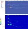 |
Fig. 13 Low Mach number case m1.5loD. Top: logarithm of gas density for times equal to 1200, 3200, and 6900 kyr or 2, 5.5, and 12 tcc. Bottom: same for the DGR with initial conditions. |
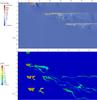 |
Fig. 14 Medium Mach number case m3loD. Top: logarithm of gas density for times equal to 600, 1700, and 2500 kyr or 2, 6, and 8 tcc. Bottom: same for the DGR. |
3.3. Formation of filaments
Our parametric survey always adopted an effective resolution of 64 cells in the original cloud radius. This was sufficient for showing the trends discussed and to demonstrate the possibility of gas-dust separation. In recent work, Lambrechts et al. (2016) analysed how a gas-dust coupled mixture, embedded in an external gravitational field, may show fine-scale development reminiscent of a streaming instability and causing filamentary dust sedimentation. In our set-up, the sudden acceleration by the passing shock can act as effective gravity, so we may expect similar filament formation to occur. To this end, we ran a higher resolution version of our reference case, m10loDzoom, with 307 cells per rc. At this resolution, we can detect additional fine structure showing up at the initial shock impact, and some selected early views on the smallest dust population d1 are given in Fig. 18 at times 0, 19.5, 39.7, and 58.7 kyr (or 0, 0.23, 0.47, and 0.70 tcc). An interesting feature is then the formation of sandbank-like structures reaching out downstream in the dust distribution, as the flow gets decelerated and deflected by the overdensity. The dust tends to deposit itself in sand piles (using a visual analogy of ripples in sandbanks), which gradually become more perpendicular to the flow. Those structures are then stretched over large distances, forming long filaments of dust as shown in Fig. 18. These filaments may well be visible in radio observations of shock-impacted clouds, which are dominated by the dust (see the next section). This proof-of-principle axisymmetric, high-resolution run would need a true 3D realization to investigate the ultimate 3D structure of these filaments to see how they appear from all direction of sights.
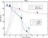 |
Fig. 15 Comparing different Mach number cases. Evolution of the mass of the cloud core and mixing region over time. The vertical line corresponds to tmix, when reached. The arrows represent the timesteps shown in Figs. 1, 13, and 14. |
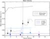 |
Fig. 16 Comparing different Mach number cases: showing mean velocity of the cloud core and mixing region. The vertical line corresponds to tmix. The arrows represent the timesteps shown in Figs. 1, 13, and 14. |
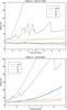 |
Fig. 17 Position of the different dust species and cloud core for m1.5loD and m3loD along the Z-axis. |
 |
Fig. 18 Case m10loDzoom, formation of sandbank, and stretching into filaments. The symmetry axis is vertical; dust population d1 is shown at times 0, 19.5, 39.7, and 58.7 kyr. |
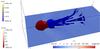 |
Fig. 19 3D representation of m10loD3D. In the 2D cut is the logarithm of the density of the gas. The smaller and larger dust population are rendered as a 3D isosurface with value 0.01. |
3.4. 3D simulation and synthetic emission maps
In previous gas-dust modelling efforts (Hendrix et al. 2015, 2016), we demonstrated that MPI-AMRVAC simulations can be directly passed on to Monte Carlo-based radiative transfer simulations by SKIRT (Camps & Baes 2015). We here use this to translate a 3D set-up of m10loD3D to a radio image, obtaining a synthetic emission map of the simulated cloud as observed from earth. Parameters for this case are as in the reference Mach 10 run, representative of an average galactic molecular cloud as extracted from the survey of Juvela et al. (2012). For the radio map, the cloud is placed at 5.5 kpc from us, placing it well within the Milky Way, and illuminated by a background plummet distribution of typical size 24 pc and total luminosity equal to 1000 times our sun. The size parameters of the dust bins (see Sect. 2) are implemented in the Skirt parameters files, and their distribution is directly imported from MPI-AMRVAC data files. We imported the octree structure from the data files, or used an octree built on the dust distribution.
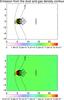 |
Fig. 20 Synthetic emission maps at time 78 kyr (0.93 tcc). Top: for a single wavelength of 5 mm. Bottom: for all wavelengths. Distances on the axes are in parsec, unit of the colour bar are in Jansky. We integrated the density over the line of sight. We show the logarithm of the resulting 2D map as black contour. Distance are in parsec (corresponding to 38 s of arc at a distance of 5.5 kpc from the source). |
Figure 19 is a 3D representation of this simulation at time 156 kyr (1.87 tcc), at the start of the mixing of the cloud. The 2D cut plane contains the logarithm of the gas density. In blue we have the volume of the smaller dust (d1) and in red the volume of the larger dust (d4) at a value of 0.01 (code unit). We see the same behaviour here as for the 2D case with the smaller dust following the gas dynamics and being caught in the instabilities, whereas the larger dust falls behind and partly shields the post-shock flow. Figures 20 and 21 are synthetic emission maps obtained with SKIRT. Figure 20 shows a map at time 78 kyr (0.93 tcc) and Fig. 21 for 156 kyr (1.87 tcc). Each time the top panel shows the emission for a single wavelength of 5 mm and the bottom panel shows the emission summed over the whole bandwidth from 0.09 μm to 10 mm. Their main difference is that the 5 mm wavelength only shows secondary emission from the dust that is warmed up by the background light to a few Kelvin on average and then radiates in the infrared. The full bandwidth view shows both light from the background and scattered light by the dust. Overplotted on the emission maps are contours of the (logarithm of the) gas density integrated over the line of sight. If we were using the simple assumption that dust and gas are located in the same region of space, these contours would coincide with the emission maps. We see this is not the case as we have a clear spatial decorrelation between the gas location and the peak of emission: the peak of density is located at 6 and 7 parsec, respectively, whereas the peak of emission is between 5 and 6 parsec for both times. We see no observable emission from the d1 dust region as it has been spread out over a large volume. Hence, also relatively early in the interaction between a strong shock and a gas-dust cloud, we would already argue for observable effects, where the dust no longer traces exactly the position of the gas. A 1 parsec separation at a distance of 5.5 kpc from the source would result in a 38 arcsec angle, which is about the resolution of the PACS instrument aboard Herschel (see Poglitsch et al. 2010).
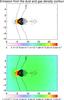 |
Fig. 21 Synthetic emission maps at time 156 kyr (1.87 tcc). Top: for a single wavelength of 5 mm. Bottom: for all wavelengths. Distances on the axes are in parsec, unit of the colour bar are in Jansky. We integrated the density over the line of sight. We show the logarithm of the resulting 2D map as black contour. Distance are in parsec (corresponding to 38 s of arc at a distance of 5.5 kpc from the source). |
4. Conclusions and discussion
The effect of dust on the dynamics of the interaction of a shock with a molecular cloud is negligible, even for large dust-to-gas ratios. As in cases without dust, the Mach number of the interacting shock plays a dominant role. This implies that we can ignore the dust in actual studies of such an interaction when the kinetics and the turbulent destruction of MCs is of interest. Dust plays other roles in the dynamics, such as being a catalyst for the occuring chemistry. We showed that a supersonic shock followed by a continuous flow, such as that produced by the wind bubble of a star, can result in a complete dissociation of the dust and gas. It can be argued that the shock would break down larger dust grains into smaller dust grains, which we found to be more likely to stay locked in the dynamics of the gas. The timescales and spatial separation observed suggest that this would not be sufficient to counteract the separation for larger grains completely. Also all dust species here are already taken as being small and under 0.5 μm. We show by means of synthetic imaging that with a realistic case for a galactic molecular cloud, the resulting infrared (dust-based) observations would give an offset position of the molecular cloud that does not fully correspond to the position of the gas of this cloud.
Many effects have been left out of our study. The radiative pressure can play a significant role if a source dominates over the background. If we assume spherical dust grains, this pressure term has a size dependency as r2 while the inertia term is volumetric and thus r3. As a result, the bigger grains are less affected than the smaller grains and gas. Furthermore, we know that dust grains get charged by interacting with ions and cosmic rays. But to which extent and on which timescale this occurs depends so much on dust composition and geometry that is it difficult to construct a simple model of its charge and, thus, of the way it interacts with the magnetic field. Therefore, the effect of the magnetic field is hard to estimate. Future work should address the role of radiative losses, combined with thermal conduction, on the simplified adiabatic simulations performed here. Incorporating the radiation field of local stars would further call for including reheating by photoionization. This may balance the radiative losses without cooling off the whole domain over a fraction of the simulation time, but can introduce even more finescale dynamics due to radiatively driven thinning of shocked shells and filaments. Properly following these processes would result in a better understanding of the thermodynamics of actual gas-dust molecular clouds.
Future studies could also explore the induced fine structure in dust distributions due to temporarily effective accelerations by shock impact, and these studies could be implemented in full 3D and translated to synthetic views. One could also make a physics-based multi-fluid model to follow populations of molecules, such as CO, and make a comparison with the gas and dust position. But this would require that we seriously follow the chemistry that takes place in this event. Similarly, it would be interesting to incorporate coalescence and destruction (as a result of the turbulence that develops) of the dust grains.
Acknowledgments
This research was supported by the Interuniversity Attraction Poles Programme by the Belgian Science Policy Office (IAP P7/08 CHARM). The simulations were conducted on the VSC (Flemish Supercomputer Center funded by Hercules foundation and Flemish government). We acknowledge financial support from project GOA/2015-014.
References
- Camps, P., & Baes, M. 2015, Astron. Comput., 9, 20 [NASA ADS] [CrossRef] [Google Scholar]
- Cha, S.-H., & Nayakshin, S. 2011, MNRAS, 415, 3319 [NASA ADS] [CrossRef] [Google Scholar]
- Draine, B. T., & Lee, H. M. 1984, ApJ, 285, 89 [Google Scholar]
- Ferrière, K. M. 2001, RvMP, 73, 1031 [Google Scholar]
- Hendrix, T., & Keppens, R. 2014, A&A, 562, A114 [NASA ADS] [CrossRef] [EDP Sciences] [Google Scholar]
- Hendrix, T., Keppens, R., & Camps, P. 2015, A&A, 575, A110 [NASA ADS] [CrossRef] [EDP Sciences] [Google Scholar]
- Hendrix, T., Keppens, R., van Marle, A. J., et al. 2016, MNRAS, 460, 3975 [NASA ADS] [CrossRef] [Google Scholar]
- Hopkins, P. F., & Lee, H. 2016, MNRAS, 456, 4174 [NASA ADS] [CrossRef] [Google Scholar]
- Johansen, A., Henning, T., & Klahr, H. 2006, ApJ, 643, 1219 [NASA ADS] [CrossRef] [Google Scholar]
- Juvela, M., Ristorcelli, I., Pagani, L., et al. 2012, A&A, 541, A12 [NASA ADS] [CrossRef] [EDP Sciences] [Google Scholar]
- Keppens, R., Meliani, Z., Marle, A. J. V., et al. 2012, JCoPh, 231, 718 [Google Scholar]
- Kwok, S. 1975, ApJ, 198, 583 [NASA ADS] [CrossRef] [Google Scholar]
- Laibe, G., & Price, D. J. 2012, MNRAS, 420, 2345 [NASA ADS] [CrossRef] [Google Scholar]
- Lambrechts, M., Johansen, A., Capelo, H. L., Blum, J., & Bodenschatz, E. 2016, A&A, 591, A133 [NASA ADS] [CrossRef] [EDP Sciences] [Google Scholar]
- Lilley, A. E. 1955, ApJ, 121, 559 [NASA ADS] [CrossRef] [Google Scholar]
- Meheut, H., Meliani, Z., Varniere, P., & Benz, W. 2012, A&A, 545, A134 [NASA ADS] [CrossRef] [EDP Sciences] [Google Scholar]
- Miniati, F. 2010, J. Comput. Phys., 229, 3916 [NASA ADS] [CrossRef] [Google Scholar]
- Nakamura, F., McKee, C. F., Klein, R. I., & Fisher, R. T. 2006, ApJS, 164, 477 [NASA ADS] [CrossRef] [Google Scholar]
- Paardekooper, S.-J., & Mellema, G. 2006, A&A, 450, 1203 [NASA ADS] [CrossRef] [EDP Sciences] [Google Scholar]
- Pittard, J. M., Falle, S. A. E. G., Hartquist, T. W., & Dyson, J. E. 2009, MNRAS, 394, 1351 [NASA ADS] [CrossRef] [Google Scholar]
- Pittard, J. M., Hartquist, T. W., & Falle, S. A. E. G. 2010, MNRAS, 405, 821 [NASA ADS] [Google Scholar]
- Poglitsch, A., Waelkens, C., Geis, N., et al. 2010, A&A, 518, L2 [NASA ADS] [CrossRef] [EDP Sciences] [Google Scholar]
- Porth, O., Xia, C., Hendrix, T., Moschou, S. P., & Keppens, R. 2014, ApJS, 214, 4 [Google Scholar]
- Roman-Duval, J., Israel, F. P., Bolatto, A., et al. 2010, A&A, 518, L74 [NASA ADS] [CrossRef] [EDP Sciences] [Google Scholar]
- Schure, K. M., Kosenko, D., Kaastra, J. S., Keppens, R., & Vink, J. 2009, A&A, 508, 751 [NASA ADS] [CrossRef] [EDP Sciences] [Google Scholar]
- van Marle, A. J., Meliani, Z., Keppens, R., & Decin, L. 2011, ApJ, 734, L26 [NASA ADS] [CrossRef] [Google Scholar]
All Tables
All Figures
|
Fig. 1 For case m10loD. Top: logarithm of gas density for times 100, 200, 540, and 700 kyr. These times correspond to a first, second, and third interaction peak, and the post-mixing phase. The symmetry axis is horizontal. Bottom: views on the dust-to-gas ratio (DGR) for the same times (and for our initial condition). |
| In the text | |
|
Fig. 2 For case m10noD, i.e. the case without dust. Logarithm of the gas density for times equal to 100, 200, 600, and 700 kyr, corresponding to the first, second, and third interaction peak, and post-mixing phase. The symmetry axis is horizontal. |
| In the text | |
|
Fig. 3 Comparing m10loD with m10noD. Top: evolution of the mass of the cloud core and the mixing region over time. The vertical line corresponds to tmix. The arrows represent the timesteps shown in Figs. 1 and 2. Bottom: evolution of the maximal Z reach of the shocked interstellar medium (SISM) and of the mixing region, together with both maximal and miminal cloud core position. |
| In the text | |
|
Fig. 4 Comparing m10loD with m10noD. Top: mean velocity of the cloud core and in the mixing region. The vertical line corresponds to tmix. The arrows represent the timesteps shown in Figs. 1 and 2. Bottom: kinetic energy evolution of the cloud core. |
| In the text | |
|
Fig. 5 Position of the different dust species and cloud core for m10loD along the Z-axis. |
| In the text | |
|
Fig. 6 R and Z component of the drag force applied to the d2 dust population. |
| In the text | |
|
Fig. 7 Zoom in for case m10loD, following the blob of dust population d2 for time 310, 470, 630, and 780 kyr. The blob gets deformed and compacted before assuming a wing shape and being stretched in both the R and Z direction. The symmetry axis is vertical. |
| In the text | |
|
Fig. 8 Case m10meD. Top: logarithm of gas density for t equal to 100, 200, 540, and 700 kyr. Bottom: same for the dust-to-gas ratio but with initial conditions. |
| In the text | |
|
Fig. 9 Case m10hiD. Top: logarithm of gas density for t equal to 100, 220, 650, and 700 kyr. Bottom: same for the DGR, with initial conditions. |
| In the text | |
|
Fig. 10 Comparing varying dust ratios. Top: evolution of the mass of the cloud core and mixing region over time. The vertical lines correspond to tmix. The arrows represent the timesteps shown in Figs. 1, 8, and 9. Bottom: evolution of the maximal Z reach of the shocked interstellar medium (SISM), mixing region, maximal cloud core position, and minimal cloud core position. |
| In the text | |
|
Fig. 11 Comparing varying dust ratios. Top: mean velocity of the cloud core and mixing region. The vertical lines correspond to tmix. The arrows represent the timesteps shown in Figs. 1, 8, and 9. Bottom: kinetic energy of the cloud core. |
| In the text | |
|
Fig. 12 Comparison of the position of the two smaller dust species in m10loD, m10meD, and m10hiD along the Z-axis. Top is species d1 (average 1.66 × 10⁻³μm) and bottom species d2 (average size 5.9 × 10⁻²μm). |
| In the text | |
|
Fig. 13 Low Mach number case m1.5loD. Top: logarithm of gas density for times equal to 1200, 3200, and 6900 kyr or 2, 5.5, and 12 tcc. Bottom: same for the DGR with initial conditions. |
| In the text | |
|
Fig. 14 Medium Mach number case m3loD. Top: logarithm of gas density for times equal to 600, 1700, and 2500 kyr or 2, 6, and 8 tcc. Bottom: same for the DGR. |
| In the text | |
|
Fig. 15 Comparing different Mach number cases. Evolution of the mass of the cloud core and mixing region over time. The vertical line corresponds to tmix, when reached. The arrows represent the timesteps shown in Figs. 1, 13, and 14. |
| In the text | |
|
Fig. 16 Comparing different Mach number cases: showing mean velocity of the cloud core and mixing region. The vertical line corresponds to tmix. The arrows represent the timesteps shown in Figs. 1, 13, and 14. |
| In the text | |
|
Fig. 17 Position of the different dust species and cloud core for m1.5loD and m3loD along the Z-axis. |
| In the text | |
|
Fig. 18 Case m10loDzoom, formation of sandbank, and stretching into filaments. The symmetry axis is vertical; dust population d1 is shown at times 0, 19.5, 39.7, and 58.7 kyr. |
| In the text | |
|
Fig. 19 3D representation of m10loD3D. In the 2D cut is the logarithm of the density of the gas. The smaller and larger dust population are rendered as a 3D isosurface with value 0.01. |
| In the text | |
|
Fig. 20 Synthetic emission maps at time 78 kyr (0.93 tcc). Top: for a single wavelength of 5 mm. Bottom: for all wavelengths. Distances on the axes are in parsec, unit of the colour bar are in Jansky. We integrated the density over the line of sight. We show the logarithm of the resulting 2D map as black contour. Distance are in parsec (corresponding to 38 s of arc at a distance of 5.5 kpc from the source). |
| In the text | |
|
Fig. 21 Synthetic emission maps at time 156 kyr (1.87 tcc). Top: for a single wavelength of 5 mm. Bottom: for all wavelengths. Distances on the axes are in parsec, unit of the colour bar are in Jansky. We integrated the density over the line of sight. We show the logarithm of the resulting 2D map as black contour. Distance are in parsec (corresponding to 38 s of arc at a distance of 5.5 kpc from the source). |
| In the text | |
Current usage metrics show cumulative count of Article Views (full-text article views including HTML views, PDF and ePub downloads, according to the available data) and Abstracts Views on Vision4Press platform.
Data correspond to usage on the plateform after 2015. The current usage metrics is available 48-96 hours after online publication and is updated daily on week days.
Initial download of the metrics may take a while.