© ESO, 2017

1. Introduction

Time-distance helioseismology and related techniques are methods for probing the complex dynamics of the solar convection zone (Duvall et al. 1993; Gizon & Birch 2005; Gizon et al. 2010). Information is encoded at the solar surface in the two-point cross-covariance function of the random solar oscillations. The cross-covariance function tells us about the travel time of wave packets between any two locations, in either direction. Flows break the time-symmetry of the cross-covariance function and thus leave a signature in the observations.

Two topics of current interest include the study of meridional circulation (e.g., Zhao et al. 2013; Liang & Chou 2015) and convective flows (e.g., Hanasoge et al. 2012; Langfellner et al. 2015) using, in particular, the SDO/HMI space observations. In both cases, low flow velocities are involved, resulting in travel-time perturbations that are less than a second. Hence it is not surprising that answers vary among investigators as they choose different interpretations and modeling procedures (for a review see Hanasoge et al. 2016).

Helioseismic studies consist of several steps: measuring solar oscillations, processing and averaging the observations to extract the seismic data (e.g., wave travel times), and interpreting the seismic data using forward and inverse methods to estimate solar internal properties. In this paper we mostly consider the forward problem, i.e. the computation of synthetic seismic data for a given solar model, which is a necessary step for reliable interpretations. A short discussion of the iterative inverse problem is given at the end of the paper.

A framework was proposed by Gizon & Birch (2002) to compute perturbations to the cross-covariance function caused by weak heterogeneities. This framework has proven to be useful for local helioseismology (Birch et al. 2004, 2007; Birch & Gizon 2007; Jackiewicz et al. 2008; Švanda et al. 2011; Hanasoge et al. 2011; Burston et al. 2015; Böning et al. 2016). However, the computational expense has been a limiting factor in applications. Advances in the fields of Earth seismology, exploration geophysics and ocean acoustics provide some guidance for improvements of the computational methods and the PDE-constrained formulations of the forward and inverse methods. Hanasoge et al. (2011) took a step in the direction of incorporating some of these ideas in the time domain within the framework of Gizon & Birch (2002). Of particular relevance to the present work is the proposal by Nissen-Meyer et al. (2014) to consider 3D wave propagation in relevant axisymmetric background media, in order to reduce the computational cost. Using a spectral decomposition in the azimuthal direction, the forward problem separates into many independent 2D problems, which can be solved to study the spatial sensitivity of seismic travel times to 3D heterogeneities (van Driel & Nissen-Meyer 2014; van Driel et al. 2015; Bottero et al. 2016). In addition, theoretical studies have led to a better understanding of the connection between the cross-covariance function and the Green’s function in media permeated by random sources of excitation (Snieder & Larose 2013, and references therein).

In this paper we consider a number of current challenges for computational local helioseismology and propose some solutions. Some of these challenges are listed here:

• Oscillation power spectrum. The purpose of helioseismology isto infer a model for the solar interior (density, sound speed, flows,etc., as functions of position) that is consistent with the seismicdata. In global mode helioseismology, the emphasis is on thecomparison between the model and observed mode frequencies.In contrast, local helioseismology requires models for the modeamplitudes and line profiles in addition to the mode frequen-cies. Thus a solar model must also describe wave excitation anddamping. Most reference solar models are 1D and their qualitycan be assessed by comparing the model and observed oscillationpower spectra. In linear inversions for local helioseismology, thereference oscillation power spectrum has to be very solar-like.

• Flexibility. The semi-analytical methods used so far to solve the forward problem (Gizon & Birch 2002) have proved useful (e.g., Burston et al. 2015) but lack flexibility. To first order (first Born approximation), the perturbation to the cross-covariance function is given by interaction integrals over products of Green’s functions. Various approximations are made to speed up the computation of these integrals, for example using a local Cartesian geometry and neglecting some anisotropic effects. A generalization to more realistic setups, including the treatment of various instrumental (e.g., varying point-spread function) and geometrical effects (e.g., foreshortening, line-of-sight projection) is very cumbersome (e.g., Jackiewicz et al. 2007). How to include these complex effects in forward models in a reliable and efficient way is an open question.

• Representation of the Green’s function. Often Green’s functions are computed using a normal-mode expansion (Birch et al. 2004). This approach is problematic for a heterogeneous 3D reference model, for which eigenmodes are not readily available. Even if they were known, the summation formula would be computationally expensive. An additional complication is the treatment of the continuous spectrum above the acoustic cutoff frequency (5.3 mHz).

• Time-domain simulations. Alternatively, the Green’s function may be computed numerically by solving the equations of motion in the time domain (e.g., Hanasoge & Duvall 2007; Cameron et al. 2008). However, this requires a stabilization of the background model by changing the buoyancy frequency (e.g., Schunker et al. 2011; Papini et al. 2014). Unless this operation is performed first, the linearized equations allow convective modes that grow exponentially. Unfortunately the mode frequencies are seriously affected by the stabilization of the solar model and move too far from the solar observations (Papini et al. 2014).

• Computational challenge and inverse problem. Modern helioseismic observations consist of large data sets (long time series of 16 megapixel images). Cross-correlations span a huge 5D space. Extracting the relevant information from this data set requires a good strategy and an efficient forward solver. This is especially true for iterative inversions, in which the forward solver is run for each update of the model of the solar interior.

We propose to address the above issues by carrying out the following steps:

• Rewriting the perturbation to the cross-covariance function interms of the Green’s function, G, and the expectation value of thecross-covariance function, $\overline{\mathit{C}}$, in the reference model. In thisformalism G and $\overline{\mathit{C}}$ are the fundamental quantities that enter anyforward calculation in local helioseismology. The problem thenbecomes deterministic. Additionally, many systematic effectscan be accounted for by treating them as numerical operations on Gand $\overline{\mathit{C}}$.

• Computing G and $\overline{\mathit{C}}$ in the frequency-domain. The advantage of this approach is that frequencies are independent of each other for wave propagation in a steady background (many important problems in helioseismology fall in this category). This allows trivial parallelization of the computation in a multi-core environment. Furthermore, the computation can easily be restricted to the frequency range of interest, at the necessary frequency resolution.

• Adopting a flexible geometrical setup using a finite-element discretization of the problem. This will enable us to treat problems in which the required spatial resolution depends on both the vertical and horizontal coordinates. Spherical geometry is naturally possible in this setup.

• Considering a simplified problem of scalar acoustics in a stratified axially symmetric reference model for the sake of simplicity. Because of the axial symmetry the problem separates into many independent 2D problems, one for each azimuthal order. The parallelization in both frequency and azimuthal order allows very efficient computation.

• Demonstrating that there is a choice of source covariance such that the expectation value of the cross-covariance is directly related to the Green’s function, even in the presence of a background flow. In this setting, the Green’s function is the only fundamental quantity that needs to be computed.

We use the above approach to compute model power spectra, time-distance diagrams, and travel-time sensitivity kernels. An application including a large-scale meridional flow will be presented. Even though we consider a scalar observable in this paper, the proposed approach is intended to be generalized to more realistic observables in the future.

2. Pure acoustics in the frequency domain

2.1. Solar oscillations

In an inertial frame, the displacement ξ(r,t) of small amplitude waves obeys an equation of the form ${\left(\frac{\mathit{\partial }}{\mathit{\partial t}}\mathrm{+}\mathit{\gamma }\mathrm{\otimes }\mathrm{+}{u}\mathrm{·}\mathrm{\nabla }\right)}^{\mathrm{2}}{\xi }\mathrm{+}\mathrm{\mathscr{H}}\mathrm{\left[}{\xi }\mathrm{\right]}\mathrm{=}{f}\mathit{,}$(1)where ℋ is a spatial operator and u(r) is a background flow. Wave attenuation is accounted for by temporal convolution (⊗) with the function γ(r,t). The function f(r,t) represents forcing by turbulent convection and is thus a realization drawn from a random process. The spatial differential operator ℋ is Hermitian for appropriate choices of the boundary condition and inner product (see Lynden-Bell & Ostriker 1967). An approximation of ℋ that captures the physics of acoustic oscillations is: $\mathrm{\mathscr{H}}\mathrm{\left[}{\xi }\mathrm{\right]}\mathrm{=}\mathrm{-}\frac{\mathrm{1}}{\mathit{\rho }}\mathrm{\nabla }\mathrm{(}\mathit{\rho }{\mathit{c}}^{\mathrm{2}}\mathrm{\nabla }\mathrm{·}{\xi }\mathrm{)}\mathrm{+}\mathrm{termsinvolvinggravity}\mathit{,}$(2)where ρ and c are the density and sound speed in the reference model. Assuming that the medium is steady, the problem can be written in frequency space as $\mathrm{-}\mathrm{(}\mathit{\omega }\mathrm{+}\mathrm{i}\hspace{0.17em}\begin{array}{c}\mathrm{􏽢}\\ \mathit{\gamma }\end{array}\mathrm{+}\mathrm{i}{u}\mathrm{·}\mathrm{\nabla }{\mathrm{)}}^{\mathrm{2}}\hspace{0.17em}\begin{array}{c}\mathrm{􏽢}\\ {\xi }\end{array}\mathrm{+}\mathrm{\mathscr{H}}\mathrm{[}\begin{array}{c}\mathrm{􏽢}\\ {\xi }\end{array}\mathrm{]}\mathrm{=}\begin{array}{c}\mathrm{􏽢}\\ {f}\end{array}\mathit{,}$(3)using the Fourier convention $\begin{array}{c}\mathrm{􏽢}\\ {\xi }\end{array}\mathrm{\left(}{r}\mathit{,\omega }\mathrm{\right)}\mathrm{=}\frac{\mathrm{1}}{\mathrm{2}\mathit{\pi }}{\mathrm{\int }}_{\mathrm{-}\mathrm{\infty }}^{\mathrm{\infty }}{\xi }\mathrm{\left(}{r}\mathit{,t}\mathrm{\right)}\hspace{0.17em}{\mathrm{e}}^{\mathrm{i}\mathit{\omega t}}\hspace{0.17em}\mathrm{d}\mathit{t}\mathit{.}$(4)If, in addition, the source of excitation is statistically stationary, then the frequency components $\begin{array}{c}{}^{\mathrm{􏽢}}\\ {f}\end{array}\mathrm{\left(}{r}\mathit{,\omega }\mathrm{\right)}$ are independent random variables and the frequency components of the wave displacement, $\begin{array}{c}{}^{\mathrm{􏽢}}\\ {\xi }\end{array}\mathrm{\left(}{r}\mathit{,\omega }\mathrm{\right)}$, are also statistically independent of each other. Thus, in frequency space, the problem separates into a set of independent boundary-value problems, one for each frequency.

In the following sections we drop the hat on top of Fourier transforms to simplify the notation.

2.2. Scalar wave equation

We further specify the wave equation to be solved. There are two possible choices for reducing the equation for the wave displacement to a scalar equation. One possibility is to rewrite Eq. (3)in terms of the quantity ψ = c∇·ξ. Neglecting the gravity terms, the second-order terms in γ and u, and the cross term in γu in Eq. (3), and then taking the divergence, we obtain $\begin{array}{ccc}& & \mathrm{-}\mathrm{(}{\mathit{\omega }}^{\mathrm{2}}\mathrm{+}\mathrm{2}\mathrm{i}\mathit{\omega \gamma }\mathrm{)}\mathit{\psi }\mathrm{-}\mathrm{2}\mathrm{i}\mathit{\omega c}\hspace{0.17em}\mathrm{\nabla }\mathrm{·}\left({u}\mathrm{·}\mathrm{\nabla }{\xi }\right)\mathrm{-}\mathrm{2}\mathrm{i}\mathit{\omega c}\hspace{0.17em}{\xi }\mathrm{·}\mathrm{\nabla }\mathit{\gamma }\\ & & \mathrm{-}\mathit{c}\mathrm{\nabla }\mathrm{·}\left(\frac{\mathrm{1}}{\mathit{\rho }}\mathrm{\nabla }\left(\mathit{\rho c\psi }\right)\right)\mathrm{=}\mathit{c}\mathrm{\nabla }\mathrm{·}{f}\mathit{.}\end{array}$(5)For slow variations of u, c and γ compared to the wavelength, the wave equation for ψ simplifies to $\mathit{L}\mathrm{\left[}\mathit{\psi }\mathrm{\right]}\mathrm{:}\mathrm{=}\mathrm{-}{\mathit{\sigma }}^{\mathrm{2}}\mathit{\psi }\mathrm{-}\mathrm{2}\mathrm{i}\mathit{\omega }\hspace{0.17em}{u}\mathrm{·}\mathrm{\nabla }\mathit{\psi }\mathrm{+}\mathit{H}\mathrm{\left[}\mathit{\psi }\mathrm{\right]}\mathrm{=}\mathit{s}$(6)with $\begin{array}{ccc}\hspace{0.17em}\begin{array}{c}\begin{array}{c}\end{array}{\mathit{\sigma }}^{\mathrm{2}}\mathrm{:}\mathrm{=}{\mathit{\omega }}^{\mathrm{2}}\mathrm{+}\mathrm{2}\mathrm{i}\mathit{\omega \gamma }\begin{array}{c}\end{array}\\ \begin{array}{c}\end{array}\mathit{H}\mathrm{\left[}\mathit{\psi }\mathrm{\right]}\mathrm{:}\mathrm{=}\mathrm{-}\mathit{c}\mathrm{\nabla }\mathrm{·}\left(\frac{\mathrm{1}}{\mathit{\rho }}\mathrm{\nabla }\mathrm{\left(}\mathit{\rho c\psi }\mathrm{\right)}\right)\mathit{.}\end{array}& & \end{array}$(7)The random source of excitation, s(r,ω) = c(r)∇·f(r,ω), and the attenuation, γ(r,ω) > 0, depend on frequency.

Another possible choice in order to obtain a scalar equation is to use the ansatz ξ = ρ^-1∇(ρcψ). Under the assumption that the forcing term ρf is curl free, this leads to the same scalar equation as above.

When ρ and c are solar-like, the scalar Eq. (6)captures most of the interesting physics of p modes. For example, a solar-like density gives the correct acoustic cutoff frequency of 5.3 mHz. However, this equation is not relevant for modeling f and g modes.

Here, we choose to specify the source of excitation through the covariance function $\mathit{M}\mathrm{\left(}{r}\mathit{,}{r}\mathrm{\prime }\mathit{,\omega }\mathrm{\right)}\mathrm{=}E\mathrm{\left[}{\mathit{s}}^{\mathrm{\ast }}\mathrm{\right(}{r}\mathit{,\omega }\mathrm{\left)}\mathit{s}\mathrm{\right(}{r}\mathrm{\prime }\mathit{,\omega }\mathrm{\left)}\mathrm{\right]}\mathrm{=}\mathit{ϵ}\mathrm{\left(}{r}\mathrm{\right)}\mathrm{\Pi }\mathrm{\left(}\mathit{\omega }\mathrm{\right)}\mathit{\delta }\mathrm{(}{r}\mathrm{-}{r}\mathrm{\prime }\mathrm{)}\mathit{,}$(8)where ∗ takes the complex conjugate and the functions ϵ(r) and Π(ω) control the spatial and frequency dependencies of the source covariance respectively. In the above expression we assumed spatially uncorrelated sources. This formulation is standard in local helioseismology (e.g., Birch et al. 2004).

2.3. Boundary condition

The geometrical setup is shown in Fig. 1. We work in a spherical-polar coordinate system (r,θ,φ). The solar (or stellar) model is cylindrically symmetric around the ẑ-axis. The computational boundary S encloses the solar photosphere. The wave equation is supplemented by a boundary condition at S on ψ. We denote by the unit normal vector to S and by ∂_nψ the normal derivative of ψ.

A free-surface boundary condition (ψ ∝ ∇·ξ = 0, Dirichlet) is often used in helioseismology (Bogdan et al. 1996; Christensen-Dalsgaard 2003, etc.). However, it is more appropriate to choose a transparent boundary condition to model the continuous spectrum above 5.3 mHz and to allow high-frequency waves to escape (e.g., Kumar et al. 1990). The use of perfectly matched layers is one way to approximate a transparent boundary (e.g., Hanasoge et al. 2011). Here, we choose the simplest approximation to the Sommerfeld outgoing radiation condition, ${\mathit{\partial }}_{\mathit{n}}\mathit{\psi }\mathrm{=}\mathrm{i}{\mathit{k}}_{\mathit{n}}\mathit{\psi } \mathrm{on}\mathit{S,}$(9)where k_n is the local wavenumber normal to the boundary. In order for this radiation boundary condition to hold true, the sound speed and density must be constant near the computational boundary, which is not the case in the Sun. In practice, we extend the solar reference model with a layer that smoothly transitions to constant density and sound speed (see Sect. 7.1 for details).

2.4. Hermiticity

In this section and the following, we demonstrate some important properties of the scalar wave Eq. (6), which will be used in the later sections. These basic properties would remain the same in the full vector equations.

One important property of the equations that describe non-attenuating waves in the Sun is the Hermiticity of the wave operator, which implies that the eigenvalues are real. Lynden-Bell & Ostriker (1967) proved Hermiticity of the wave operator for a self-gravitating fluid bounded by a free surface.

Here we ask if this condition is satisfied for the time-harmonic scalar wave equation defined by Eq. (6). The scalar wave field belongs to a complex Hilbert space. For any two functions ψ and ϕ in this space we define the inner product $\mathrm{⟨}\mathit{\psi ,\varphi }\mathrm{⟩}\mathrm{=}{\mathrm{\int }}_{\mathit{V}}{\mathit{\psi }}^{\mathrm{\ast }}\mathit{\varphi }\hspace{0.17em}\mathit{\rho }\mathrm{d}{r}\mathit{,}$(10)where V is the computational domain. Performing integration by parts twice implies $\mathrm{⟨}\mathit{\psi ,H}\mathrm{\left[}\mathit{\varphi }\mathrm{\right]}\mathrm{⟩}\mathrm{=}\mathrm{⟨}\mathit{H}\mathrm{\left[}\mathit{\psi }\mathrm{\right]}\mathit{,\varphi }\mathrm{⟩}\mathrm{-}{\mathrm{\int }}_{\mathit{S}}\left[{\mathit{\psi }}^{\mathrm{\ast }}\hspace{0.17em}{\mathit{\partial }}_{\mathit{n}}\mathrm{\left(}\mathit{\rho c\varphi }\mathrm{\right)}\mathrm{-}\mathit{\varphi }\hspace{0.17em}{\mathit{\partial }}_{\mathit{n}}\mathrm{\left(}\mathit{\rho c}{\mathit{\psi }}^{\mathrm{\ast }}\mathrm{\right)}\right]\mathit{c}\hspace{0.17em}\mathrm{d}\mathit{S}\mathit{.}$(11)We see that the spatial operator H is Hermitian if ψ and ϕ vanish on the boundary. However, for a radiation boundary condition, the surface integral remains and H is not Hermitian. The eigenvalues of H are no longer real.

The other terms in Eq. (6)are the damping and advection terms. Using integration by parts once, we ascertain that the damping operator is anti-Hermitian and the advection operator is Hermitian: $\begin{array}{ccc}& & \mathrm{⟨}\mathit{\psi ,}\mathrm{2}\mathrm{i}\mathit{\omega \gamma \varphi }\mathrm{⟩}\mathrm{=}\mathrm{-}\mathrm{⟨}\mathrm{2}\mathrm{i}\mathit{\omega \gamma \psi ,\varphi }\mathrm{⟩}\mathit{,}\\ & & \mathrm{⟨}\mathit{\psi ,}\mathrm{2}\mathrm{i}\mathit{\omega }{u}\mathrm{·}\mathrm{\nabla }\mathit{\varphi }\mathrm{⟩}\mathrm{=}\mathrm{⟨}\mathrm{2}\mathrm{i}\mathit{\omega }{u}\mathrm{·}\mathrm{\nabla }\mathit{\psi ,\varphi }\mathrm{⟩}\mathit{.}\end{array}$The last result is a consequence of mass conservation, ∇·(ρu) = 0, for a steady flow that does not cross the computational boundary ( on S).

Combining Eqs. (6), and (11)–(13)yields $\mathrm{⟨}\mathit{\psi ,L}\mathrm{\left[}\mathit{\varphi }\mathrm{\right]}\mathrm{⟩}\mathrm{=}\mathrm{⟨}{\mathit{L}}^{†}\mathrm{\left[}\mathit{\psi }\mathrm{\right]}\mathit{,\varphi }\mathrm{⟩}\mathrm{-}{\mathrm{\int }}_{\mathit{S}}\left[{\mathit{\psi }}^{\mathrm{\ast }}{\mathit{\partial }}_{\mathit{n}}\left(\mathit{\rho c\varphi }\right)\mathrm{-}\mathit{\varphi }{\mathit{\partial }}_{\mathit{n}}\mathrm{\left(}\mathit{\rho c}{\mathit{\psi }}^{\mathrm{\ast }}\mathrm{\right)}\right]\mathit{c}\hspace{0.17em}\mathrm{d}\mathit{S,}$(14)where ${\mathit{L}}^{†}\mathrm{=}{\mathit{L}}_{\mathrm{(}\mathrm{-}\mathit{\gamma }\mathrm{)}}\mathrm{=}{\mathit{L}}_{\mathrm{(}\mathrm{-}{u}\mathrm{)}}^{\mathrm{\ast }}$(15)is the operator obtained by switching the sign of γ in L or, equivalently, by switching the sign of u and taking the complex conjugate. We note that for a radiation boundary condition, L^† is not the adjoint of L because the surface integral remains.

2.5. Green’s function and generalized seismic reciprocity

In geophysics, the principle of seismic reciprocity states that the same signal should be recorded if the locations of a source and a receiver are exchanged. Although seismic reciprocity is not preserved in the presence of a flow, a generalization of reciprocity can be obtained.

Let us introduce the Green’s function as the solution to $\mathit{L}\mathrm{\left[}\mathit{G}\mathrm{\right(}{r}\mathit{,}{r}\mathrm{\prime }\mathit{,\omega }\mathrm{\left)}\mathrm{\right]}\mathrm{=}\frac{\mathrm{1}}{\mathit{\rho }\mathrm{\left(}{r}\mathrm{\right)}}\mathit{\delta }\mathrm{(}{r}\mathrm{-}{r}\mathrm{\prime }\mathrm{)}\mathit{,}$(16)where δ is the Dirac delta function and G satisfies the same boundary condition as the wave field ψ. Consider a source at r₁ in the physical domain and a source at r₂ in the domain in which the flow has opposite sign: $\begin{array}{ccc}\{\hspace{0.17em}\begin{array}{c}\begin{array}{c}\end{array}\mathit{\rho }\hspace{0.17em}\mathit{L}\mathrm{\left[}\mathit{G}\mathrm{\right(}{r}\mathit{,}{r}\mathrm{1}\mathit{,\omega }\mathrm{\left)}\mathrm{\right]}\mathrm{=}\mathit{\delta }\mathrm{(}{r}\mathrm{-}{r}\mathrm{1}\mathrm{)}\begin{array}{c}\end{array}\\ \begin{array}{c}\end{array}\mathit{\rho }\hspace{0.17em}{\mathit{L}}_{\mathrm{(}\mathrm{-}{u}\mathrm{)}}\mathrm{\left[}\mathit{G}\mathrm{\right(}{r}\mathit{,}{r}\mathrm{2}\mathit{,\omega }\mathrm{;}\mathrm{-}{u}\mathrm{\left)}\mathrm{\right]}\mathrm{=}\mathit{\delta }\mathrm{(}{r}\mathrm{-}{r}\mathrm{2}\mathrm{)}\mathit{,}\end{array}& & \end{array}$(17)where G(·;−u) is the Green’s function associated with the operator L_{(− u)}, with the same boundary condition as G. Multiplying the first equation by G(r,r₂,ω;−u) and the second by G(r,r₁,ω), integrating each over position r, and subtracting the two equations, we obtain $\begin{array}{ccc}\hspace{0.17em}\begin{array}{c}\begin{array}{c}\end{array}\mathit{G}\mathrm{(}{r}\mathrm{1}\mathit{,}{r}\mathrm{2}\mathit{,\omega }\mathrm{;}\mathrm{-}{u}\mathrm{)}\mathrm{-}\mathit{G}\mathrm{\left(}{r}\mathrm{2}\mathit{,}{r}\mathrm{1}\mathit{,\omega }\mathrm{\right)}\mathrm{=}\begin{array}{c}\end{array}\\ \begin{array}{c}\end{array} ⟨{\mathit{G}}^{\mathrm{\ast }}\mathrm{(}{r}\mathit{,}{r}\mathrm{2}\mathit{,\omega }\mathrm{;}\mathrm{-}{u}\mathrm{)}\mathit{,L}\mathrm{\left[}\mathit{G}\mathrm{\right(}{r}\mathit{,}{r}\mathrm{1}\mathit{,\omega }\mathrm{\left)}\mathrm{\right]}⟩\\ \begin{array}{c}\end{array} \mathrm{-}\mathrm{⟨}{\mathit{L}}^{†}\mathrm{\left[}{\mathit{G}}^{\mathrm{\ast }}\mathrm{\right(}{r}\mathit{,}{r}\mathrm{2}\mathit{,\omega }\mathrm{;}\mathrm{-}{u}\mathrm{\left)}\mathrm{\right]}\mathit{,G}\mathrm{\left(}{r}\mathit{,}{r}\mathrm{1}\mathit{,\omega }\mathrm{\right)}\mathrm{⟩}\mathit{.}\end{array}& & \end{array}$(18)Following the same logic as earlier (integration by parts), $\mathrm{⟨}{\mathit{\psi }}^{\mathrm{\ast }}\mathit{,L}\mathrm{\left[}\mathit{\varphi }\mathrm{\right]}\mathrm{⟩}\mathrm{=}\mathrm{⟨}{\mathit{L}}^{†}\mathrm{\left[}{\mathit{\psi }}^{\mathrm{\ast }}\mathrm{\right]}\mathit{,\varphi }\mathrm{⟩}\mathrm{-}{\mathrm{\int }}_{\mathit{S}}\left[\mathit{\psi }{\mathit{\partial }}_{\mathit{n}}\left(\mathit{\rho c\varphi }\right)\mathrm{-}\mathit{\varphi }{\mathit{\partial }}_{\mathit{n}}\left(\mathit{\rho c\psi }\right)\right]\mathit{c}\mathrm{d}\mathit{S}$(19)for any two functions ψ and ϕ in the space of solutions. This time the surface integral vanishes for either type of boundary condition (Dirichlet or radiation). In particular, $\mathrm{⟨}{\mathit{L}}^{†}\mathrm{\left[}{\mathit{G}}^{\mathrm{\ast }}\mathrm{\right]}\mathit{,\varphi }\mathrm{⟩}\mathrm{=}⟨{\mathit{G}}^{\mathrm{\ast }}\mathit{,L}\mathrm{\left[}\mathit{\varphi }\mathrm{\right]}⟩\mathit{.}$(20)This relationship shows that the right-hand side of Eq. (18)vanishes and so we find $\mathit{G}\mathrm{\left(}{r}\mathrm{2}\mathit{,}{r}\mathrm{1}\mathit{,\omega }\mathrm{\right)}\mathrm{=}\mathit{G}\mathrm{(}{r}\mathrm{1}\mathit{,}{r}\mathrm{2}\mathit{,\omega }\mathrm{;}\mathrm{-}{u}\mathrm{)}\mathit{.}$(21)This is a generalization of seismic reciprocity: the Green’s function is unchanged upon exchanging source and receiver and changing the sign of the flow. The conclusion holds even though the damping operator is not Hermitian.

3. Cross-covariance function and travel times

For the sake of simplicity, let us suppose that ψ can be directly measured on the solar surface. This choice is not unreasonable as ψ is proportional to the pressure fluctuations and is thus related to intensity fluctuations, an observable quantity. This choice is not at all a limitation of the method: other observables can be derived from ψ, for example a proxy for the line-of-sight velocity.

At frequency ω, consider the cross-covariance in Fourier space as the product of the wave field at two locations of measurement, $\begin{array}{ccc}\hspace{0.17em}\begin{array}{c}\begin{array}{c}\end{array}\mathit{C}\mathrm{\left(}{r}\mathrm{1}\mathit{,}{r}\mathrm{2}\mathit{,\omega }\mathrm{\right)}\mathrm{=}{\mathit{\psi }}^{\mathrm{\ast }}\mathrm{\left(}{r}\mathrm{1}\mathit{,\omega }\mathrm{\right)}\hspace{0.17em}\mathit{\psi }\mathrm{\left(}{r}\mathrm{2}\mathit{,\omega }\mathrm{\right)}\mathit{.}\end{array}& & \end{array}$(22)In terms of the Green’s function, we have $\mathit{\psi }\mathrm{\left(}{r}\mathit{j}\mathit{,\omega }\mathrm{\right)}\mathrm{=}{\mathrm{\int }}_{\mathit{V}}\mathit{G}\mathrm{\left(}{r}\mathit{j}\mathit{,}{r}\mathit{,\omega }\mathrm{\right)}\mathit{s}\mathrm{\left(}{r}\mathit{,\omega }\mathrm{\right)}\hspace{0.17em}\mathit{\rho }\mathrm{d}{r}\mathit{,}$(23)where the source s(r,ω) is a realization of a random process. Under the assumption of spatially uncorrelated sources (see Eq. (8)), the cross-covariance can be written as one volume integral: $\begin{array}{ccc}\hspace{0.17em}\begin{array}{c}\begin{array}{c}\end{array}\overline{\mathit{C}}\mathrm{\left(}{r}\mathrm{1}\mathit{,}{r}\mathrm{2}\mathit{,\omega }\mathrm{\right)}\mathrm{=}E\mathrm{\left[}\mathit{C}\mathrm{\right(}{r}\mathrm{1}\mathit{,}{r}\mathrm{2}\mathit{,\omega }\mathrm{\left)}\mathrm{\right]}\begin{array}{c}\end{array}\\ \begin{array}{c}\end{array} \mathrm{=}{\mathrm{\int }}_{\mathit{V}}\mathit{\rho }\mathrm{d}{r}{\mathrm{\int }}_{\mathit{V}}{\mathit{\rho }}^{\mathrm{\prime }}\mathrm{d}{r}\mathrm{\prime }{\mathit{G}}^{\mathrm{\ast }}\mathrm{\left(}{r}\mathrm{1}\mathit{,}{r}\mathit{,\omega }\mathrm{\right)}\hspace{0.17em}\mathit{G}\mathrm{\left(}{r}\mathrm{2}\mathit{,}{r}\mathrm{\prime }\mathit{,\omega }\mathrm{\right)}\hspace{0.17em}\mathit{M}\mathrm{\left(}{r}\mathit{,}{r}\mathrm{\prime }\mathit{,\omega }\mathrm{\right)}\\ \begin{array}{c}\end{array} \mathrm{=}\mathrm{\Pi }\mathrm{\left(}\mathit{\omega }\mathrm{\right)}{\mathrm{\int }}_{\mathit{V}}{\mathit{G}}^{\mathrm{\ast }}\mathrm{\left(}{r}\mathrm{1}\mathit{,}{r}\mathit{,\omega }\mathrm{\right)}\hspace{0.17em}\mathit{G}\mathrm{\left(}{r}\mathrm{2}\mathit{,}{r}\mathit{,\omega }\mathrm{\right)}\hspace{0.17em}\mathit{ϵ}\mathrm{\left(}{r}\mathrm{\right)}\hspace{0.17em}{\mathit{\rho }}^{\mathrm{2}}\mathrm{d}{r}\mathit{.}\end{array}& & \end{array}$(24)Following Gizon & Birch (2002), we define the perturbation to the travel time δτ between points r₁ and r₂ as $\mathit{\delta \tau }\mathrm{\left(}{r}\mathrm{1}\mathit{,}{r}\mathrm{2}\mathrm{\right)}\mathrm{=}{\mathrm{\int }}_{\mathrm{-}\mathrm{\infty }}^{\mathrm{\infty }}{\mathit{W}}^{\mathrm{\ast }}\mathrm{\left(}\mathit{\omega }\mathrm{\right)}\hspace{0.17em}\mathrm{\left[}\mathit{C}\mathrm{\right(}{r}\mathrm{1}\mathit{,}{r}\mathrm{2}\mathit{,\omega }\mathrm{)}\mathrm{-}{\mathit{C}}_{\mathrm{ref}}\mathrm{(}{r}\mathrm{1}\mathit{,}{r}\mathrm{2}\mathit{,\omega }\mathrm{\left)}\mathrm{\right]}\hspace{0.17em}\mathrm{d}\mathit{\omega ,}$(25)where $\mathit{W}\mathrm{\left(}\mathit{\omega }\mathrm{\right)}\mathrm{=}\mathrm{-}\frac{{\mathrm{\int }}_{\mathrm{-}\mathrm{\infty }}^{\mathrm{\infty }}\mathit{w}\mathrm{\left(}\mathit{t}\mathrm{\right)}\hspace{0.17em}\mathrm{\left[}{\mathit{\partial }}_{\mathit{t}}{\mathit{C}}_{\mathrm{ref}}\mathrm{\right(}{r}\mathrm{1}\mathit{,}{r}\mathrm{2}\mathit{,t}\mathrm{\left)}\mathrm{\right]}\hspace{0.17em}{\mathrm{e}}^{\mathrm{i}\mathit{\omega t}}\hspace{0.17em}\mathrm{d}\mathit{t}}{{\mathrm{\int }}_{\mathrm{-}\mathrm{\infty }}^{\mathrm{\infty }}\mathit{w}\mathrm{\left(}{\mathit{t}}^{\mathrm{\prime }}\mathrm{\right)}\hspace{0.17em}\mathrm{\left[}{\mathit{\partial }}_{{\mathit{t}}^{\mathrm{\prime }}}{\mathit{C}}_{\mathrm{ref}}\mathrm{\right(}{r}\mathrm{1}\mathit{,}{r}\mathrm{2}\mathit{,}{\mathit{t}}^{\mathrm{\prime }}\mathrm{)}{\mathrm{]}}^{\mathrm{2}}\hspace{0.17em}\mathrm{d}{\mathit{t}}^{\mathrm{\prime }}}\mathit{,}$(26)C_refis a reference cross-covariance function, and w(t) is a temporal window function that selects a particular section of the data. For example, we can choose w(t) = exp [−(t−t_g)²/ 2σ²] where t_g> 0 is a group time and σ sets the width of the window.

4. New formulation of travel time sensitivity kernels

In the presence of subsurface perturbations to the reference model the travel times computed from Eq. (25)will be affected. An understanding of the spatial sensitivity of the measurements to structural perturbations and flows requires the development of travel time sensitivity kernels. In this section we develop a new formulation of the travel-time sensitivity kernels in terms of the Green’s function and the cross-covariance computed in the reference model.

4.1. Perturbations to the medium

In addressing how travel times are sensitive to changes in the solar reference model, we consider changes in c(r), ρ(r), and u(r), as well as spatial changes to the attenuation γ(r) and the source amplitude ϵ(r). The vector flow ${u}\mathrm{\left(}{r}\mathrm{\right)}\mathrm{=}\sum _{\mathit{k}}{\mathit{u}}_{\mathit{k}}\mathrm{\left(}{r}\mathrm{\right)}\hspace{0.17em}{{ê}}_{\mathit{k}}\mathrm{\left(}{r}\mathrm{\right)}\mathrm{=}{\mathit{u}}_{\mathit{r}}\mathrm{\left(}{r}\mathrm{\right)}{r̂}\mathrm{+}{\mathit{u}}_{\mathit{\theta }}\mathrm{\left(}{r}\mathrm{\right)}{\theta ̂}\mathrm{+}{\mathit{u}}_{\mathit{\phi }}\mathrm{\left(}{r}\mathrm{\right)}{\phi ̂}\mathit{,}$(27)is specified by the three components u_k on the basis { ê_k } of unit vectors , and for the spherical-polar coordinate system. In short, the physical variables of interest can be combined into a set $\mathrm{\left\{}{\mathit{q}}_{\mathit{\alpha }}\mathrm{\right\}}\mathrm{=}\mathrm{\left\{}\mathit{c,\rho ,}{\mathit{u}}_{\mathit{r}}\mathit{,}{\mathit{u}}_{\mathit{\theta }}\mathit{,}{\mathit{u}}_{\mathit{\phi }}\mathit{,\gamma ,ϵ}\mathrm{\right\}}\mathit{.}$(28)We are looking for travel-time sensitivity kernels K_α such that the travel-time perturbation δτ can be written as $E\mathrm{\left[}\mathit{\delta \tau }\mathrm{\right]}\mathrm{=}\sum _{\mathit{\alpha }}{\mathrm{\int }}_{\mathit{V}}\mathit{\delta }{\mathit{q}}_{\mathit{\alpha }}\mathrm{\left(}{r}\mathrm{\right)}{\mathit{K}}_{\mathit{\alpha }}\mathrm{\left(}{r}\mathrm{\right)}\hspace{0.17em}\mathrm{d}{r}\mathrm{+}\mathrm{surfaceterms}\mathit{,}$(29)for infinitesimal perturbations δq_α. For some variables there is a surface integral on the computational boundary, because integration by parts is needed to write travel-time perturbations in the form of Eq. (29). For these variables, we assume that the perturbations to the model vanish on the computational boundary (high in the atmosphere) and we drop the surface terms.

In order to find the kernels, the travel-time perturbation $\mathit{\delta \tau }\mathrm{\left(}{r}\mathrm{1}\mathit{,}{r}\mathrm{2}\mathrm{\right)}\mathrm{=}{\mathrm{\int }}_{\mathrm{-}\mathrm{\infty }}^{\mathrm{\infty }}{\mathit{W}}^{\mathrm{\ast }}\mathrm{\left(}\mathit{\omega }\mathrm{\right)}\hspace{0.17em}\mathit{\delta C}\mathrm{\left(}{r}\mathrm{1}\mathit{,}{r}\mathrm{2}\mathit{,\omega }\mathrm{\right)}\hspace{0.17em}\mathrm{d}\mathit{\omega }$(30)is written in terms of the first-order perturbation to the cross-covariance: $\mathit{\delta C}\mathrm{\left(}{r}\mathrm{1}\mathit{,}{r}\mathrm{2}\mathit{,\omega }\mathrm{\right)}\mathrm{=}{\mathit{\psi }}^{\mathrm{\ast }}\mathrm{\left(}{r}\mathrm{1}\mathit{,\omega }\mathrm{\right)}\hspace{0.17em}\mathit{\delta \psi }\mathrm{\left(}{r}\mathrm{2}\mathit{,\omega }\mathrm{\right)}\mathrm{+}\mathit{\delta }{\mathit{\psi }}^{\mathrm{\ast }}\mathrm{\left(}{r}\mathrm{1}\mathit{,\omega }\mathrm{\right)}\hspace{0.17em}\mathit{\psi }\mathrm{\left(}{r}\mathrm{2}\mathit{,\omega }\mathrm{\right)}\mathit{.}$(31)The next step is then to express δψ in terms of the δq_α.

4.2. Perturbation to the wave field

To first order (first Born approximation) the operator defined in Eq. (6)acts on the perturbed wave field through, $\begin{array}{ccc}\mathit{L}\mathrm{\left[}\mathit{\delta \psi }\mathrm{\right]}& \mathrm{=}& \mathrm{-}\mathit{\delta L}\mathrm{\left[}\mathit{\psi }\mathrm{\right]}\mathrm{+}\mathit{\delta s}\\ & \mathrm{=}& \end{array}$(32)where δL is the perturbation to the wave operator caused by perturbations to the medium and $\begin{array}{ccc}\mathit{\delta H}\mathrm{\left[}\mathit{\psi }\mathrm{\right]}& \mathrm{=}& \frac{\mathit{\delta c}}{\mathit{c}}\mathit{H}\mathrm{\left[}\mathit{\psi }\mathrm{\right]}\mathrm{+}\mathit{H}\left[\frac{\mathit{\delta c}}{\mathit{c}}\mathit{\psi }\right]\\ & & \mathrm{-}\mathit{c}\mathrm{\nabla }\mathrm{·}\left(\frac{\mathit{\delta \rho }}{{\mathit{\rho }}^{\mathrm{2}}}\mathrm{\nabla }\mathrm{\left(}\mathit{\rho c\psi }\mathrm{\right)}\right)\mathrm{+}\mathit{H}\left[\frac{\mathit{\delta \rho }}{\mathit{\rho }}\mathit{\psi }\right]\mathrm{·}\end{array}$(33)A formal solution to Eq. (32)is obtained in terms of the Green’s function: $\begin{array}{ccc}\hspace{0.17em}\begin{array}{c}\begin{array}{c}\end{array}\mathit{\delta \psi }\mathrm{\left(}{r}\mathit{j}\mathit{,\omega }\mathrm{\right)}\mathrm{=}\mathrm{-}{\mathrm{\int }}_{\mathit{V}}\mathit{G}\mathrm{\left(}{r}\mathit{j}\mathit{,}{r}\mathit{,\omega }\mathrm{\right)}\hspace{0.17em}\mathit{\delta L}\mathrm{\left[}\mathit{\psi }\mathrm{\right(}{r}\mathit{,\omega }\mathrm{\left)}\mathrm{\right]}\hspace{0.17em}\mathit{\rho }\mathrm{d}{r}\begin{array}{c}\end{array}\\ \begin{array}{c}\end{array}\mathrm{+}{\mathrm{\int }}_{\mathit{V}}\mathit{G}\mathrm{\left(}{r}\mathit{j}\mathit{,}{r}\mathit{,\omega }\mathrm{\right)}\hspace{0.17em}\mathit{\delta s}\mathrm{\left(}{r}\mathit{,\omega }\mathrm{\right)}\hspace{0.17em}\mathit{\rho }\mathrm{d}{r}\mathit{.}\end{array}& & \end{array}$(34)

4.3. Perturbation to the cross-covariance

With Eq. (34)in hand, the expectation of the perturbation to the cross-covariance is then determined from Eq. (31): $\begin{array}{ccc}\hspace{0.17em}\begin{array}{c}\begin{array}{c}\end{array}\mathit{\delta }\overline{\mathit{C}}\mathrm{\left(}{r}\mathrm{1}\mathit{,}{r}\mathrm{2}\mathit{,\omega }\mathrm{\right)}\mathrm{=}\mathrm{-}{\mathrm{\int }}_{\mathit{V}}\mathit{G}\mathrm{\left(}{r}\mathrm{2}\mathit{,}{r}\mathit{,\omega }\mathrm{\right)}\mathit{\delta L}\mathrm{[}\overline{\mathit{C}}\mathrm{(}{r}\mathrm{1}\mathit{,}{r}\mathit{,\omega }{\mathrm{)}}^{\mathrm{]}}\hspace{0.17em}\mathit{\rho }\mathrm{d}{r}\begin{array}{c}\end{array}\\ \begin{array}{c}\end{array}\mathrm{-}{\mathrm{\int }}_{\mathit{V}}{\mathit{G}}^{\mathrm{\ast }}\mathrm{\left(}{r}\mathrm{1}\mathit{,}{r}\mathit{,\omega }\mathrm{\right)}\mathit{\delta }{\mathit{L}}^{\mathrm{\ast }}\mathrm{[}{\overline{\mathit{C}}}^{\hspace{0.17em}\mathrm{\ast }}\mathrm{(}{r}\mathrm{2}\mathit{,}{r}\mathit{,\omega }{\mathrm{)}}^{\mathrm{]}}\hspace{0.17em}\mathit{\rho }\mathrm{d}{r}\\ \begin{array}{c}\end{array}\mathrm{+}\mathrm{\Pi }\mathrm{\left(}\mathit{\omega }\mathrm{\right)}{\mathrm{\int }}_{\mathit{V}}{\mathit{G}}^{\mathrm{\ast }}\mathrm{\left(}{r}\mathrm{1}\mathit{,}{r}\mathit{,\omega }\mathrm{\right)}\mathit{G}\mathrm{\left(}{r}\mathrm{2}\mathit{,}{r}\mathit{,\omega }\mathrm{\right)}\hspace{0.17em}\mathit{\delta ϵ}\mathrm{\left(}{r}\mathrm{\right)}\hspace{0.17em}{\mathit{\rho }}^{\mathrm{2}}\mathrm{d}{r}\mathit{,}\end{array}& & \end{array}$(35)where we write the perturbation to the source covariance as a spatially varying change in amplitude, $E\mathrm{\left[}{\mathit{s}}^{\mathrm{\ast }}\mathrm{\right(}{r}\mathit{,\omega }\mathrm{\left)}\mathit{\delta s}\mathrm{\right(}{r}\mathrm{\prime }\mathit{,\omega }\mathrm{)}\mathrm{+}\mathit{\delta }{\mathit{s}}^{\mathrm{\ast }}\mathrm{(}{r}\mathit{,\omega }\mathrm{\left)}\mathit{s}\mathrm{\right(}{r}\mathrm{\prime }\mathit{,\omega }\mathrm{\left)}\mathrm{\right]}\mathrm{=}\mathit{\delta ϵ}\mathrm{\left(}{r}\mathrm{\right)}\mathrm{\Pi }\mathrm{\left(}\mathit{\omega }\mathrm{\right)}\mathit{\delta }\mathrm{(}{r}\mathrm{-}{r}\mathrm{\prime }\mathrm{)}\mathit{.}$(36)In order to obtain kernels for individual perturbations, we introduce the bilinear operators ℒ_α such that for any functions g and h we have ${\mathrm{\int }}_{\mathit{V}}\mathit{g\delta L}\mathrm{\left[}\mathit{h}\mathrm{\right]}\hspace{0.17em}\mathit{\rho }\mathrm{d}{r}\mathrm{=}\sum _{\mathit{\alpha }}{\mathrm{\int }}_{\mathit{V}}\mathit{\delta }{\mathit{q}}_{\mathit{\alpha }}\mathrm{\left(}{r}\mathrm{\right)}\hspace{0.17em}{\mathrm{ℒ}}_{\mathit{\alpha }}\mathrm{\left[}\mathit{g,h}\mathrm{\right]}\hspace{0.17em}\mathrm{d}{r}\mathrm{+}\mathrm{surfaceterms}\mathit{.}$(37)These bilinear operators are obtained by integration by parts and are explicitly given by $\begin{array}{ccc}{\mathrm{ℒ}}_{\mathit{c}}\mathrm{\left[}\mathit{g,h}\mathrm{\right]}& \mathrm{=}& \left(\mathit{g}\hspace{0.17em}\mathit{H}\mathrm{\left[}\mathit{h}\mathrm{\right]}\mathrm{+}\mathit{h}\hspace{0.17em}\mathit{H}\mathrm{\left[}\mathit{g}\mathrm{\right]}\right)\mathit{\rho }\mathit{/}\mathit{c,}\\ {\mathrm{ℒ}}_{\mathit{\rho }}\mathrm{\left[}\mathit{g,h}\mathrm{\right]}& \mathrm{=}& \mathrm{-}\mathrm{\nabla }\mathrm{\left(}\mathit{\rho cg}\mathrm{\right)}\mathrm{·}\mathrm{\nabla }\mathrm{\left(}\mathit{\rho ch}\mathrm{\right)}\mathit{/}{\mathit{\rho }}^{\mathrm{2}}\mathrm{+}\mathit{h}\hspace{0.17em}\mathit{H}\mathrm{\left[}\mathit{g}\mathrm{\right]}\mathit{,}\\ {\mathrm{ℒ}}_{{\mathit{u}}_{\mathit{k}}}\mathrm{\left[}\mathit{g,h}\mathrm{\right]}& \mathrm{=}& \\ {\mathrm{ℒ}}_{\mathit{\gamma }}\mathrm{\left[}\mathit{g,h}\mathrm{\right]}& \mathrm{=}& \mathrm{-}\mathrm{2}\mathrm{i}\mathit{\rho \omega }\hspace{0.17em}\mathit{g}\hspace{0.17em}\mathit{h}\mathit{.}\end{array}$In Eq. (40), ${\mathit{\partial }}_{\mathit{k}}\mathrm{=}\hat{{e}}{}_{\mathit{k}}\mathrm{\left(}{r}\mathrm{\right)}\mathrm{·}{\mathrm{\nabla }}_{{r}}$ denotes the component of the spatial gradient in the k direction. Combining Eqs. (37) and (35), we obtain an explicit linear relationship between the δq_α and $\mathit{\delta }\overline{\mathit{C}}$: $\begin{array}{ccc}\hspace{0.17em}\begin{array}{c}\begin{array}{c}\end{array}\mathit{\delta }\overline{\mathit{C}}\mathrm{\left(}{r}\mathrm{1}\mathit{,}{r}\mathrm{2}\mathit{,\omega }\mathrm{\right)}\mathrm{=}\begin{array}{c}\end{array}\\ \begin{array}{c}\end{array} \mathrm{-}\sum _{\mathit{\alpha }}{\mathrm{\int }}_{\mathit{V}}\mathit{\delta }{\mathit{q}}_{\mathit{\alpha }}\mathrm{\left(}{r}\mathrm{\right)}{\mathrm{ℒ}}_{\mathit{\alpha }}\mathrm{[}\mathit{G}\mathrm{\left(}{r}\mathrm{2}\mathit{,}{r}\mathit{,\omega }\mathrm{\right)}\mathit{,}\overline{\mathit{C}}\mathrm{(}{r}\mathrm{1}\mathit{,}{r}\mathit{,\omega }{\mathrm{)}}^{\mathrm{]}}\mathrm{d}{r}\\ \begin{array}{c}\end{array} \mathrm{-}\sum _{\mathit{\alpha }}{\mathrm{\int }}_{\mathit{V}}\mathit{\delta }{\mathit{q}}_{\mathit{\alpha }}\mathrm{\left(}{r}\mathrm{\right)}{\mathrm{ℒ}}_{\mathit{\alpha }}^{\mathrm{\ast }}\mathrm{[}{\mathit{G}}^{\mathrm{\ast }}\mathrm{\left(}{r}\mathrm{1}\mathit{,}{r}\mathit{,\omega }\mathrm{\right)}\mathit{,}{\overline{\mathit{C}}}^{\hspace{0.17em}\mathrm{\ast }}\mathrm{(}{r}\mathrm{2}\mathit{,}{r}\mathit{,\omega }{\mathrm{)}}^{\mathrm{]}}\mathrm{d}{r}\\ \begin{array}{c}\end{array} \mathrm{+}\mathrm{\Pi }\mathrm{\left(}\mathit{\omega }\mathrm{\right)}{\mathrm{\int }}_{\mathit{V}}\mathit{\delta ϵ}\mathrm{\left(}{r}\mathrm{\right)}\hspace{0.17em}{\mathit{G}}^{\mathrm{\ast }}\mathrm{\left(}{r}\mathrm{1}\mathit{,}{r}\mathit{,\omega }\mathrm{\right)}\mathit{G}\mathrm{\left(}{r}\mathrm{2}\mathit{,}{r}\mathit{,\omega }\mathrm{\right)}\hspace{0.17em}{\mathit{\rho }}^{\mathrm{2}}\mathrm{d}{r}\\ \begin{array}{c}\end{array} \mathrm{+}\mathrm{surfaceterms}\mathit{.}\end{array}& & \end{array}$(42)Using this expression together with Eqs. (29)and (30), the travel-time sensitivity kernels are $\begin{array}{ccc}\hspace{0.17em}\begin{array}{c}\begin{array}{c}\end{array}{\mathit{K}}_{\mathit{\alpha }}\mathrm{\left(}{r}\mathrm{;}{r}\mathrm{1}\mathit{,}{r}\mathrm{2}\mathrm{\right)}\mathrm{=}\mathrm{-}{\mathrm{\int }}_{\mathrm{-}\mathrm{\infty }}^{\mathrm{\infty }}{\mathit{W}}^{\mathrm{\ast }}\mathrm{\left(}\mathit{\omega }\mathrm{\right)}{\mathrm{ℒ}}_{\mathit{\alpha }}\mathrm{[}\mathit{G}\mathrm{\left(}{r}\mathrm{2}\mathit{,}{r}\mathit{,\omega }\mathrm{\right)}\mathit{,}\overline{\mathit{C}}\mathrm{(}{r}\mathrm{1}\mathit{,}{r}\mathit{,\omega }{\mathrm{)}}^{\mathrm{]}}\mathrm{d}\mathit{\omega }\begin{array}{c}\end{array}\\ \begin{array}{c}\end{array}\mathrm{-}{\mathrm{\int }}_{\mathrm{-}\mathrm{\infty }}^{\mathrm{\infty }}{\mathit{W}}^{\mathrm{\ast }}\mathrm{\left(}\mathit{\omega }\mathrm{\right)}{\mathrm{ℒ}}_{\mathit{\alpha }}^{\mathrm{\ast }}\mathrm{[}{\mathit{G}}^{\mathrm{\ast }}\mathrm{\left(}{r}\mathrm{1}\mathit{,}{r}\mathit{,\omega }\mathrm{\right)}\mathit{,}{\overline{\mathit{C}}}^{\hspace{0.17em}\mathrm{\ast }}\mathrm{(}{r}\mathrm{2}\mathit{,}{r}\mathit{,\omega }{\mathrm{)}}^{\mathrm{]}}\mathrm{d}\mathit{\omega }\end{array}& & \end{array}$(43)for the scatterers δq_α ∈ { δc,δρ,δu_k,δγ } and ${\mathit{K}}_{\mathit{ϵ}}\mathrm{\left(}{r}\mathrm{;}{r}\mathrm{1}\mathit{,}{r}\mathrm{2}\mathrm{\right)}\mathrm{=}{\mathit{\rho }}^{\mathrm{2}}\mathrm{\left(}{r}\mathrm{\right)}{\mathrm{\int }}_{\mathrm{-}\mathrm{\infty }}^{\mathrm{\infty }}\mathrm{\Pi }\mathrm{\left(}\mathit{\omega }\mathrm{\right)}{\mathit{W}}^{\mathrm{\ast }}\mathrm{\left(}\mathit{\omega }\mathrm{\right)}\hspace{0.17em}{\mathit{G}}^{\mathrm{\ast }}\mathrm{\left(}{r}\mathrm{1}\mathit{,}{r}\mathit{,\omega }\mathrm{\right)}\mathit{G}\mathrm{\left(}{r}\mathrm{2}\mathit{,}{r}\mathit{,\omega }\mathrm{\right)}\hspace{0.17em}\mathrm{d}\mathit{\omega }$(44)for the source amplitude δϵ.

5. Convenient source of excitation

5.1. How can we simplify the computation of $\overline{\mathit{C}}$?

The kernels from the previous section are well defined once the background medium, attenuation and source functions have been specified. At each ω, the attenuation function γ(r,ω) can be tuned to yield the observed line widths of solar oscillations in the power spectrum. Similarly, at each ω, the source function ϵ(r)Π(ω) can be tuned to give the observed mode amplitudes (Birch et al. 2004; Birch & Gizon 2007). However, the integral relationship between a general ϵ(r) and $\overline{\mathit{C}}$ is far from trivial to compute.

Here we adopt a different strategy. We ask whether a convenient source covariance exists such that the expectation value of the cross-covariance can be written in terms of the Green’s function. As a second step we check whether the resulting power spectrum is solar-like.

It is known in geophysics and acoustics that, under appropriate conditions on the source covariance, the expectation value of the cross-covariance in the frequency domain is related to the imaginary part of the Green’s function (see Snieder et al. 2009, and references therein). If we could write such a simple relationship, our problem would be considerably simpler. For all practical purposes, the Green’s function would be the only truly important quantity.

Let us start by rewriting the equation for the Green’s function (Eq. (16)) for sources at r₁ and r₂, taking the complex conjugate of the first: $\begin{array}{ccc}\{\hspace{0.17em}\begin{array}{c}\begin{array}{c}\end{array}\mathit{\delta }\mathrm{(}{r}\mathrm{-}{r}\mathrm{1}\mathrm{)}\mathrm{=}\mathit{\rho }\mathrm{\left(}{r}\mathrm{\right)}\hspace{0.17em}{\mathit{L}}^{\mathrm{\ast }}\mathrm{\left[}{\mathit{G}}^{\mathrm{\ast }}\mathrm{\right(}{r}\mathit{,}{r}\mathrm{1}\mathit{,\omega }\mathrm{\left)}\mathrm{\right]}\mathit{,}\begin{array}{c}\end{array}\\ \begin{array}{c}\end{array}\mathit{\delta }\mathrm{(}{r}\mathrm{-}{r}\mathrm{2}\mathrm{)}\mathrm{=}\mathit{\rho }\mathrm{\left(}{r}\mathrm{\right)}\hspace{0.17em}\mathit{L}\mathrm{\left[}\mathit{G}\mathrm{\right(}{r}\mathit{,}{r}\mathrm{2}\mathit{,\omega }\mathrm{\left)}\mathrm{\right]}\mathit{.}\end{array}& & \end{array}$(45)Multiply the first equation by G(r,r₂,ω) and the second equation by G^∗(r,r₁,ω), integrate each over r, and then subtract to find $\begin{array}{ccc}\hspace{0.17em}\begin{array}{c}\begin{array}{c}\end{array}\mathit{G}\mathrm{\left(}{r}\mathrm{1}\mathit{,}{r}\mathrm{2}\mathit{,\omega }\mathrm{\right)}\mathrm{-}{\mathit{G}}^{\mathrm{\ast }}\mathrm{\left(}{r}\mathrm{2}\mathit{,}{r}\mathrm{1}\mathit{,\omega }\mathrm{\right)}\mathrm{=}\begin{array}{c}\end{array}\\ \begin{array}{c}\end{array} \mathrm{⟨}\mathit{L}\mathrm{\left[}\mathit{G}\mathrm{\right(}{r}\mathit{,}{r}\mathrm{1}\mathit{,\omega }\mathrm{\left)}\mathrm{\right]}\mathit{,G}\mathrm{\left(}{r}\mathit{,}{r}\mathrm{2}\mathit{,\omega }\mathrm{\right)}\mathrm{⟩}\mathrm{-}\mathrm{⟨}\mathit{G}\mathrm{\left(}{r}\mathit{,}{r}\mathrm{1}\mathit{,\omega }\mathrm{\right)}\mathit{,L}\mathrm{\left[}\mathit{G}\mathrm{\right(}{r}\mathit{,}{r}\mathrm{2}\mathit{,\omega }\mathrm{\left)}\mathrm{\right]}\mathrm{⟩}\\ \begin{array}{c}\end{array} \mathrm{=}\mathrm{⟨}\mathit{L}\mathrm{\left[}\mathit{G}\mathrm{\right(}{r}\mathit{,}{r}\mathrm{1}\mathit{,\omega }\mathrm{\left)}\mathrm{\right]}\mathit{,G}\mathrm{\left(}{r}\mathit{,}{r}\mathrm{2}\mathit{,\omega }\mathrm{\right)}\mathrm{⟩}\mathrm{-}\mathrm{⟨}{\mathit{L}}^{†}\mathrm{\left[}\mathit{G}\mathrm{\right(}{r}\mathit{,}{r}\mathrm{1}\mathit{,\omega }\mathrm{\left)}\mathrm{\right]}\mathit{,G}\mathrm{\left(}{r}\mathit{,}{r}\mathrm{2}\mathit{,\omega }\mathrm{\right)}\mathrm{⟩}\\ \begin{array}{c}\end{array} \mathrm{+}\mathrm{surfaceterm}\\ \begin{array}{c}\end{array} \mathrm{=}\mathrm{4}\mathrm{i}\mathit{\omega }\mathrm{⟨}\mathit{\gamma }\mathrm{\left(}{r}\mathit{,\omega }\mathrm{\right)}\mathit{G}\mathrm{\left(}{r}\mathit{,}{r}\mathrm{1}\mathit{,\omega }\mathrm{\right)}\mathit{,G}\mathrm{\left(}{r}\mathit{,}{r}\mathrm{2}\mathit{,\omega }\mathrm{\right)}\mathrm{⟩}\mathrm{+}\mathrm{surfaceterm}\\ \begin{array}{c}\end{array} \mathrm{=}\mathrm{4}\mathrm{i}\mathit{\omega }\mathrm{⟨}\mathit{\gamma }\mathrm{\left(}{r}\mathit{,\omega }\mathrm{\right)}\mathit{G}\mathrm{(}{r}\mathrm{1}\mathit{,}{r}\mathit{,\omega }\mathrm{;}\mathrm{-}{u}\mathrm{)}\mathit{,G}\mathrm{(}{r}\mathrm{2}\mathit{,}{r}\mathit{,\omega }\mathrm{;}\mathrm{-}{u}\mathrm{)}\mathrm{⟩}\mathrm{+}\mathrm{surfaceterm}\mathrm{.}\end{array}& & \end{array}$(46)The surface term does not vanish unless specific boundary conditions are used, as noted earlier by Snieder (2007). In the solar case (transparent boundary condition), this surface term does not vanish. Reversing the flow u in the above equation, we obtain $\begin{array}{ccc}\hspace{0.17em}\begin{array}{c}\begin{array}{c}\end{array}\mathit{G}\mathrm{\left(}{r}\mathrm{2}\mathit{,}{r}\mathrm{1}\mathit{,\omega }\mathrm{\right)}\mathrm{-}{\mathit{G}}^{\mathrm{\ast }}\mathrm{(}{r}\mathrm{2}\mathit{,}{r}\mathrm{1}\mathit{,\omega }\mathrm{;}\mathrm{-}{u}\mathrm{)}\mathrm{=}\begin{array}{c}\end{array}\\ \begin{array}{c}\end{array} \mathrm{4}\mathrm{i}\mathit{\omega }{\mathrm{\int }}_{\mathit{V}}\mathit{\gamma }\mathrm{\left(}{r}\mathit{,\omega }\mathrm{\right)}{\mathit{G}}^{\mathrm{\ast }}\mathrm{\left(}{r}\mathrm{1}\mathit{,}{r}\mathit{,\omega }\mathrm{\right)}\mathit{G}\mathrm{\left(}{r}\mathrm{2}\mathit{,}{r}\mathit{,\omega }\mathrm{\right)}\hspace{0.17em}\mathit{\rho }\mathrm{d}\mathit{V}\\ \begin{array}{c}\end{array} \hspace{0.17em}\hspace{0.17em}\hspace{0.17em}\hspace{0.17em}\mathrm{+}\mathrm{2}\mathrm{i}\mathit{\omega }{\mathrm{\int }}_{\mathit{S}}\mathit{c}\mathrm{\left(}{r}\mathrm{\right)}{\mathit{G}}^{\mathrm{\ast }}\mathrm{\left(}{r}\mathrm{1}\mathit{,}{r}\mathit{,\omega }\mathrm{\right)}\mathit{G}\mathrm{\left(}{r}\mathrm{2}\mathit{,}{r}\mathit{,\omega }\mathrm{\right)}\hspace{0.17em}\mathit{\rho }\mathrm{d}\mathit{S,}\end{array}& & \end{array}$(47)where the surface integral is the explicit expression for the surface term. By inspection of Eq. (24), we see that the choice of source covariance amplitude $\mathit{ϵ}\mathrm{:}\mathrm{=}\frac{\mathit{\gamma }\mathrm{\left(}{r}\mathit{,\omega }\mathrm{\right)}}{\mathit{\rho }\mathrm{\left(}{r}\mathrm{\right)}}\mathrm{+}\frac{\mathit{c}}{\mathrm{2}\mathit{\rho }}\mathit{\delta }\mathrm{(}\mathit{r}\mathrm{-}\mathit{R}\mathrm{(}\mathit{\theta }\mathrm{\left)}\mathrm{\right)}$(48)implies $E\mathrm{\left[}\mathit{C}\mathrm{\right(}{r}\mathrm{1}\mathit{,}{r}\mathrm{2}\mathit{,\omega }\mathrm{\left)}\mathrm{\right]}\mathrm{=}\frac{\mathrm{\Pi }\mathrm{\left(}\mathit{\omega }\mathrm{\right)}}{\mathrm{4}\mathrm{i}\mathit{\omega }}\left[\mathit{G}\mathrm{\left(}{r}\mathrm{2}\mathit{,}{r}\mathrm{1}\mathit{,\omega }\mathrm{\right)}\mathrm{-}{\mathit{G}}^{\mathrm{\ast }}\mathrm{(}{r}\mathrm{2}\mathit{,}{r}\mathrm{1}\mathit{,\omega }\mathrm{;}\mathrm{-}{u}\mathrm{)}\right]\mathit{.}$(49)Thus the expectation value of the cross-variance can be written as a sum of causal and anti-causal Green’s functions, when waves are appropriately excited throughout the volume and on the computational boundary S at radius r = R(θ). The volume sources must be proportional to the local attenuation to enforce energy equipartition between the modes (see, e.g., Snieder 2007).

To simplify the problem it would be very nice to assume that equality (49)holds. Does it give a reasonable oscillation power spectrum? The power spectrum can be tuned in frequency space by choosing Π(ω). However, the source of Eq. (48)leaves no freedom for the distribution of power versus radial order at fixed frequency.

A drawback of the choice of source (Eq. (48)) is that the source covariance cannot be updated independently from attenuation and density. Thus, perturbations to the cross-covariance are fully specified by perturbations to c, ρ, γ, and u.

5.2. Sensitivity kernels in terms of G only

As the cross-covariance depends only on the Green’s function via Eq. (49), it is also the case for the kernels. Denoting for simplicity $\begin{array}{ccc}\hspace{0.17em}\begin{array}{c}\begin{array}{c}\end{array}{\mathit{G}}_{\mathit{i}}\mathrm{\left(}{r}\mathrm{\right)}\mathrm{:}\mathrm{=}\mathit{G}\mathrm{\left(}{r}\mathit{,}{r}\mathit{i}\mathit{,\omega }\mathrm{\right)}\mathit{,}\begin{array}{c}\end{array}\\ \begin{array}{c}\end{array}{\mathit{G}}_{\mathit{i}}^{†}\mathrm{\left(}{r}\mathrm{\right)}\mathrm{:}\mathrm{=}{\mathit{G}}^{\mathrm{\ast }}\mathrm{(}{r}\mathit{,}{r}\mathit{i}\mathit{,\omega }\mathrm{;}\mathrm{-}{u}\mathrm{)}\mathit{,}\end{array}& & \end{array}$(50)the kernels defined by Eq. (43)can be computed from four Green’s functions ${\mathit{G}}_{\mathrm{1}}\mathrm{\left(}{r}\mathrm{\right)}\mathit{,}{\mathit{G}}_{\mathrm{2}}\mathrm{\left(}{r}\mathrm{\right)} \mathrm{and} {\mathit{G}}_{\mathrm{1}}^{†}\mathrm{\left(}{r}\mathrm{\right)}\mathit{,}{\mathit{G}}_{\mathrm{2}}^{†}\mathrm{\left(}{r}\mathrm{\right)}\mathit{.}$(51)For example, the travel-time perturbations induced by a background flow perturbation, $\mathit{\delta \tau }\mathrm{\left(}{r}\mathrm{1}\mathit{,}{r}\mathrm{2}\mathrm{\right)}\mathrm{=}\sum _{\mathit{k}}{\mathrm{\int }}_{\mathit{V}}\mathit{\delta }{\mathit{u}}_{\mathit{k}}\mathrm{\left(}{r}\mathrm{\right)}\hspace{0.17em}{\mathit{K}}_{{\mathit{u}}_{\mathit{k}}}\mathrm{\left(}{r}\mathrm{;}{r}\mathrm{1}\mathit{,}{r}\mathrm{2}\mathrm{\right)}\hspace{0.17em}\mathrm{d}{r}\mathit{,}$(52)can be computed through the kernels ${\mathit{K}}_{{\mathit{u}}_{\mathit{k}}}\mathrm{=}\frac{\mathit{\rho }}{\mathrm{2}}{\mathrm{\int }}_{\mathrm{-}\mathrm{\infty }}^{\mathrm{\infty }}\mathrm{\Pi }{\mathit{W}}^{\mathrm{\ast }}\left[{\mathit{G}}_{\mathrm{2}}^{†\mathrm{\ast }}{\mathit{\partial }}_{\mathit{k}}\left({\mathit{G}}_{\mathrm{1}}\mathrm{-}{\mathit{G}}_{\mathrm{1}}^{†}\right)\mathrm{+}{\mathit{G}}_{\mathrm{1}}^{†}{\mathit{\partial }}_{\mathit{k}}\left({\mathit{G}}_{\mathrm{2}}^{\mathrm{\ast }}\mathrm{-}{\mathit{G}}_{\mathrm{2}}^{†\mathrm{\ast }}\right)\right]\hspace{0.17em}\mathrm{d}\mathit{\omega }\mathit{.}$(53)

5.3. Special case of no background flow

Following from the previous section and taking the further assumption of no background flow (u = 0), seismic reciprocity implies that G^† = G^∗ and the cross-covariance takes the simple form, ${\overline{\mathit{C}}}_{\mathit{i}}\mathrm{\left(}{r}\mathrm{\right)}\mathrm{:}\mathrm{=}\overline{\mathit{C}}\mathrm{\left(}{r}\mathit{i}\mathit{,}{r}\mathit{,\omega }\mathrm{\right)}\mathrm{=}\frac{\mathrm{\Pi }\mathrm{\left(}\mathit{\omega }\mathrm{\right)}}{\mathrm{2}\mathit{\omega }}\mathrm{Im}{\mathit{G}}_{\mathit{i}}\mathrm{\left(}{r}\mathrm{\right)}\mathit{.}$(54)This simple form for the cross-covariance simplifies the scattering bilinear operators: $\begin{array}{ccc}{\mathrm{ℒ}}_{\mathit{c}}\mathrm{\left[}{\mathit{G}}_{\mathit{i}}\mathit{,}{\overline{\mathit{C}}}_{\mathit{j}}\mathrm{\right]}& \mathrm{=}& \frac{\mathit{\rho }\mathrm{\Pi }}{\mathrm{2}\mathit{\omega c}}\mathrm{[}{\mathit{G}}_{\mathit{i}}\hspace{0.17em}\mathrm{Im}\mathrm{\left(}\mathit{H}\mathrm{\right[}{\mathit{G}}_{\mathit{j}}\mathrm{\left]}\mathrm{\right)}\mathrm{+}\mathit{H}\mathrm{\left[}{\mathit{G}}_{\mathit{i}}\mathrm{\right]}\hspace{0.17em}\mathrm{Im}{\mathit{G}}_{\mathit{j}}\mathrm{]}\mathit{,}\\ {\mathrm{ℒ}}_{\mathit{\rho }}\mathrm{\left[}{\mathit{G}}_{\mathit{i}}\mathit{,}{\overline{\mathit{C}}}_{\mathit{j}}\mathrm{\right]}& \mathrm{=}& \mathrm{-}\frac{\mathrm{\Pi }}{\mathrm{2}\mathit{\omega }}\left(\frac{\mathrm{1}}{{\mathit{\rho }}^{\mathrm{2}}}\mathrm{\nabla }\mathrm{\left(}\mathit{\rho c}{\mathit{G}}_{\mathit{i}}\mathrm{\right)}\mathrm{·}\mathrm{\nabla }\mathrm{\left(}\mathit{\rho c}\hspace{0.17em}\mathrm{Im}{\mathit{G}}_{\mathit{j}}\mathrm{\right)}\mathrm{-}\mathit{H}\mathrm{\left[}{\mathit{G}}_{\mathit{i}}\mathrm{\right]}\hspace{0.17em}\mathrm{Im}{\mathit{G}}_{\mathit{j}}\right)\mathit{,}\\ & & \\ {\mathrm{ℒ}}_{{\mathit{u}}_{\mathit{k}}}\mathrm{\left[}{\mathit{G}}_{\mathit{i}}\mathit{,}{\overline{\mathit{C}}}_{\mathit{j}}\mathrm{\right]}& \mathrm{=}& \mathrm{-}\mathrm{i}\mathit{\rho }\mathrm{\Pi }\hspace{0.17em}{\mathit{G}}_{\mathit{i}}\hspace{0.17em}{\mathit{\partial }}_{\mathit{k}}\mathrm{\left(}\mathrm{Im}{\mathit{G}}_{\mathit{j}}\mathrm{\right)}\mathit{,}\\ {\mathrm{ℒ}}_{\mathit{\gamma }}\mathrm{\left[}{\mathit{G}}_{\mathit{i}}\mathit{,}{\overline{\mathit{C}}}_{\mathit{j}}\mathrm{\right]}& \mathrm{=}& \end{array}$Thus, to compute a kernel K_α when there is no background flow, all we need is two Green’s function computations, one with a source at r₁ and the other with a source at r₂.

6. Forward solver in the frequency domain

With the theory of the previous sections in hand, we wish to compute the Green’s function at fixed ω, defined by Eq. (16). In order to achieve this we utilize a standard Finite Element Method (FEM), which is further explained in Sect. 6.5.

Ideally we would solve for the Green’s function in a general 3D computational domain. However, as discussed later in Sect. 8.3, 3D computations are very demanding. In the following subsections we consider a reference model that is symmetric about an axis. This setup is appropriate for studying the effects of large-scale flows (differential rotation and meridional flow) on solar oscillations. A substantial benefit of this choice is that the solution to the 3D problem can be obtained by decomposition into a set of independent 2D problems, one for each Fourier component in longitude. We refer to problems where the background medium is axisymmetric as 2.5D problems. Below we describe the computational setup and give a weak formulation of the solved equations.

6.1. Montjoie finite element code

We utilize the FEM code Montjoie¹, developed at Inria for various wave propagation problems. Montjoie is versatile, well-tested, and robust (see Duruflé 2006; Bergot et al. 2010). Montjoie allows us to consider 1.5D, 2.5D, and 3D geometries. The 1.5D problem assumes a spherically symmetric background model and the solution is decomposed into spherical harmonics and 1D finite radial elements. The 2.5D method assumes an axisymmetric background model and the solution is decomposed into azimuthal Fourier modes and 2D finite elements; it is fast and useful for a number of applications. The full 3D method is slow, although it would work for a small fraction of the solar volume. The computational times for the respective geometries are compared in Sect. 8.3.

6.2. Geometrical setup for the 2.5D problem

For an axisymmetric background model, the computational domain Σ is a meridional generating section of the geometry (Fig. 2), i.e. the half-disk of radius R in the case of the sphere.

The background model is symmetric about the ẑ-axis. In 3D space a spatial point is associated with the position vector ${r}\mathrm{=}\mathrm{\left(}\mathit{r,\theta ,\phi }\mathrm{\right)}\mathrm{=}\mathrm{:}\mathrm{\left(}\begin{array}{c}\mathrm{˜}\\ {r}\end{array}\mathit{,\phi }\mathrm{\right)}\mathit{,}$(59)where $\begin{array}{c}{\mathrm{˜}}_{}\\ {r}\end{array}$ belongs to the 2D section Σ and φ is longitude about the axis of symmetry (Fig. 2). The background density, sound speed, and flow are specified at positions $\begin{array}{c}{\mathrm{˜}}_{}\\ {r}\end{array}$ in Σ: $\begin{array}{ccc}\mathit{\rho }& \mathrm{=}& \mathit{\rho }\mathrm{\left(}\begin{array}{c}\mathrm{˜}\\ {r}\end{array}\mathrm{\right)}\mathit{,}\\ \mathit{c}& \mathrm{=}& \mathit{c}\mathrm{\left(}\begin{array}{c}\mathrm{˜}\\ {r}\end{array}\mathrm{\right)}\mathit{,}\\ {u}& \mathrm{=}& \begin{array}{c}\mathrm{˜}\\ {u}\end{array}\mathrm{\left(}\begin{array}{c}\mathrm{˜}\\ {r}\end{array}\mathrm{\right)}\mathrm{+}{\mathit{u}}_{\mathit{\phi }}\mathrm{\left(}\begin{array}{c}\mathrm{˜}\\ {r}\end{array}\mathrm{\right)}{\phi ̂}\mathit{,}\end{array}$where $\begin{array}{c}{\mathrm{˜}}_{}\\ {u}\end{array}$ is the meridional component of the flow and u_φ the rotational velocity component.

6.3. Expansion of solution in longitudinal Fourier modes

As the unknown of the finite element method we choose the function $\begin{array}{c}{\mathrm{ˇ}}_{}\\ \mathit{\psi }\end{array}$ defined by $\begin{array}{c}\mathrm{ˇ}\\ \mathit{\psi }\end{array}\mathrm{=}\mathit{\rho c}\hspace{0.17em}\mathit{\psi }\mathit{.}$(63)The factor ρc removes the gradients of ρ or c from the weak form of the equation and thus improves convergence (see Sect. 6.5). The equation solved by $\begin{array}{c}{\mathrm{ˇ}}_{}\\ \mathit{\psi }\end{array}$ is $\mathrm{-}\frac{{\mathit{\sigma }}^{\mathrm{2}}}{\mathit{\rho }\hspace{0.17em}{\mathit{c}}^{\mathrm{2}}}\hspace{0.17em}\begin{array}{c}\mathrm{ˇ}\\ \mathit{\psi }\end{array}\mathrm{-}\frac{\mathrm{2}\mathrm{i}\mathit{\omega }}{\mathit{c}}\hspace{0.17em}{u}\mathrm{·}\mathrm{\nabla }\left(\frac{\begin{array}{c}\mathrm{ˇ}\\ \mathit{\psi }\end{array}}{\mathit{\rho c}}\right)\mathrm{-}\mathrm{\nabla }\mathrm{·}\left(\frac{\mathrm{1}}{\mathit{\rho }}\mathrm{\nabla }\begin{array}{c}\mathrm{ˇ}\\ \mathit{\psi }\end{array}\right)\mathrm{=}\frac{\mathit{s}}{\mathit{c}}\mathrm{·}$(64)In order to use the 2.5D solver, the 3D solution $\begin{array}{c}{\mathrm{ˇ}}_{}\\ \mathit{\psi }\end{array}$ must be expanded as a Fourier series in the longitudinal direction: $\begin{array}{c}\mathrm{ˇ}\\ \mathit{\psi }\end{array}\mathrm{\left(}{r}\mathit{,\omega }\mathrm{\right)}\mathrm{=}\sum _{\mathit{m}\mathrm{=}\mathrm{-}\mathrm{\infty }}^{\mathrm{\infty }}\begin{array}{c}\mathrm{ˇ}\\ {\mathit{\psi }}^{\mathit{m}}\end{array}\mathrm{\left(}\begin{array}{c}\mathrm{˜}\\ {r}\end{array}\mathit{,\omega }\mathrm{\right)}{\mathrm{e}}^{\mathrm{i}\mathit{m\phi }}\mathit{.}$(65)Inserting the above expansion into Eq. (64), we see that the 3D problem separates into a set of independent 2D problems, one for each m: $\mathrm{-}{\mathit{\sigma }}_{\mathit{m}}^{\mathrm{2}}\frac{\begin{array}{c}\mathrm{ˇ}\\ {\mathit{\psi }}^{\mathit{m}}\end{array}}{\mathit{\rho }{\mathit{c}}^{\mathrm{2}}}\mathrm{-}\frac{\mathrm{2}\mathrm{i}\mathit{\omega }}{\mathit{c}}\begin{array}{c}\mathrm{˜}\\ {u}\end{array}\mathrm{·}\begin{array}{c}\mathrm{˜}\\ \mathrm{\nabla }\end{array}\left(\frac{\begin{array}{c}\mathrm{ˇ}\\ {\mathit{\psi }}^{\mathit{m}}\end{array}}{\mathit{\rho c}}\right)\mathrm{-}\begin{array}{c}\mathrm{˜}\\ \mathrm{\nabla }\end{array}\mathrm{·}\left(\frac{\mathrm{1}}{\mathit{\rho }}\begin{array}{c}\mathrm{˜}\\ \mathrm{\nabla }\end{array}\begin{array}{c}\mathrm{ˇ}\\ {\mathit{\psi }}^{\mathit{m}}\end{array}\right)\mathrm{=}\frac{{\mathit{s}}^{\mathit{m}}}{\mathit{c}}\mathit{,}$(66)with ${\mathit{\sigma }}_{\mathit{m}}^{\mathrm{2}}\mathrm{=}{\mathit{\omega }}^{\mathrm{2}}\mathrm{+}\mathrm{2}\mathrm{i}\mathit{\omega \gamma }\mathrm{-}\frac{\mathrm{2}\mathit{m\omega }\hspace{0.17em}{\mathit{u}}_{\mathit{\phi }}}{\mathit{\varpi }}\mathrm{-}\frac{{\mathit{m}}^{\mathrm{2}}{\mathit{c}}^{\mathrm{2}}}{{\mathit{\varpi }}^{\mathrm{2}}}$(67)and ${\mathit{s}}^{\mathit{m}}\mathrm{\left(}\begin{array}{c}\mathrm{˜}\\ {r}\end{array}\mathit{,\omega }\mathrm{\right)}\mathrm{=}\frac{\mathrm{1}}{\mathrm{2}\mathit{\pi }}{\mathrm{\int }}_{\mathrm{0}}^{\mathrm{2}\mathit{\pi }}\mathit{s}\mathrm{\left(}{r}\mathit{,\omega }\mathrm{\right)}\hspace{0.17em}{\mathrm{e}}^{\mathrm{-}\mathrm{i}\mathit{m\phi }}\hspace{0.17em}\mathrm{d}\mathit{\phi }\mathit{.}$(68)The 2D gradient and divergence operators are defined by $\begin{array}{ccc}\hspace{0.17em}\begin{array}{c}\begin{array}{c}\end{array}\begin{array}{c}\mathrm{˜}\\ \mathrm{\nabla }\end{array}\mathit{F}\mathrm{=}\mathit{\varpi ̂}{\mathit{\partial }}_{\mathit{\varpi }}\mathit{F}\mathrm{+}{ẑ}{\mathit{\partial }}_{\mathit{z}}\mathit{F,}\begin{array}{c}\end{array}\\ \begin{array}{c}\end{array}\begin{array}{c}\mathrm{˜}\\ \mathrm{\nabla }\end{array}\mathrm{·}{F}\mathrm{=}\frac{\mathrm{1}}{\mathit{\varpi }}{\mathit{\partial }}_{\mathit{\varpi }}\mathrm{\left(}\mathit{\varpi }{\mathit{F}}_{\mathit{\varpi }}\mathrm{\right)}\mathrm{+}{\mathit{\partial }}_{\mathit{z}}{\mathit{F}}_{\mathit{z}}\mathit{.}\end{array}& & \end{array}$(69)On the outer boundary, we apply a Sommerfeld-like boundary condition ${\mathit{\partial }}_{\mathit{n}}\begin{array}{c}\mathrm{ˇ}\\ {\mathit{\psi }}^{\mathit{m}}\end{array}\mathrm{=}\mathrm{i}\frac{{\mathit{\sigma }}_{\mathit{m}}}{\mathit{c}}\begin{array}{c}\mathrm{ˇ}\\ {\mathit{\psi }}^{\mathit{m}}\end{array}\mathit{.}$(70)A boundary condition that would take into account the fast variation of density near the surface (exponential decay) would be preferable, thus removing the need for an extended atmosphere and resultant mesh; this will be studied in a future paper.

6.4. Expansion of Green’s function

For a delta function source at position ${r}{}_{\mathit{s}}\mathrm{=}\mathrm{\left(}{\begin{array}{c}{}_{\mathrm{˜}}\\ {r}\end{array}}_{\mathit{s}}\mathit{,}{\mathit{\phi }}_{\mathit{s}}\mathrm{\right)}$, $\mathit{s}\mathrm{\left(}{r}\mathrm{;}{r}\mathrm{s}\mathrm{\right)}\mathrm{=}\mathit{\delta }\mathrm{(}\mathit{\phi }\mathrm{-}{\mathit{\phi }}_{\mathit{s}}\mathrm{)}\hspace{0.17em}\mathit{\delta }\mathrm{(}\begin{array}{c}\mathrm{˜}\\ {r}\end{array}\mathrm{-}{\begin{array}{c}\mathrm{˜}\\ {r}\end{array}}_{\mathit{s}}\mathrm{)}\mathit{,}$(71)and the source coefficients are ${\mathit{s}}^{\mathit{m}}\mathrm{\left(}\begin{array}{c}\mathrm{˜}\\ {r}\end{array}\mathrm{;}{{r}}_{\mathit{s}}\mathrm{\right)}\mathrm{=}\{\begin{array}{c}\\ \frac{\mathrm{1}}{\mathrm{2}\mathit{\pi }}{\mathrm{e}}^{\mathrm{-}\mathrm{i}\mathit{m}{\mathit{\phi }}_{\mathit{s}}}\mathit{\delta }\mathrm{(}\begin{array}{c}\mathrm{˜}\\ {r}\end{array}\mathrm{-}{\begin{array}{c}\mathrm{˜}\\ {r}\end{array}}_{\mathit{s}}\mathrm{)}\mathrm{if}{r}\mathit{s}\mathrm{isnotonthe}{ẑ}\mathrm{axis,}\\ \frac{\mathrm{1}}{\mathrm{2}\mathit{\pi }}{\mathit{\delta }}_{\mathit{m,}\mathrm{0}}\hspace{0.17em}\mathit{\delta }\mathrm{(}\begin{array}{c}\mathrm{˜}\\ {r}\end{array}\mathrm{-}{\begin{array}{c}\mathrm{˜}\\ {r}\end{array}}_{\mathit{s}}\mathrm{)}\mathrm{otherwise}\mathrm{.}\end{array}$(72)Thus the Green’s function may be computed using $\begin{array}{c}\mathrm{ˇ}\\ \mathit{G}\end{array}\mathrm{\left(}{r}\mathit{,}{r}\mathrm{s}\mathit{,\omega }\mathrm{\right)}\mathrm{=}\sum _{\mathit{m}\mathrm{=}\mathrm{-}\mathrm{\infty }}^{\mathrm{\infty }}\begin{array}{c}\mathrm{ˇ}\\ {\mathit{G}}^{\mathit{m}}\end{array}\mathrm{\left(}\begin{array}{c}\mathrm{˜}\\ {r}\end{array}\mathit{,}{\begin{array}{c}\mathrm{˜}\\ {r}\end{array}}_{\mathit{s}}\mathit{,\omega }\mathrm{\right)}{\mathrm{e}}^{\mathrm{i}\mathit{m}\mathrm{(}\mathit{\phi }\mathrm{-}{\mathit{\phi }}_{\mathit{s}}\mathrm{)}}\mathrm{=}\mathit{\rho }\mathrm{\left(}\begin{array}{c}\mathrm{˜}\\ {r}\end{array}\mathrm{\right)}\mathit{c}\mathrm{\left(}\begin{array}{c}\mathrm{˜}\\ {r}\end{array}\mathrm{\right)}\mathit{G}\mathrm{\left(}{r}\mathit{,}{r}\mathrm{s}\mathit{,\omega }\mathrm{\right)}\mathit{,}$(73)where each $\begin{array}{c}{\mathrm{ˇ}}_{}\\ {\mathit{G}}^{\mathit{m}}\end{array}$ solves $\mathrm{-}{\mathit{\sigma }}_{\mathit{m}}^{\mathrm{2}}\frac{\begin{array}{c}\mathrm{ˇ}\\ {\mathit{G}}^{\mathit{m}}\end{array}}{\mathit{\rho }{\mathit{c}}^{\mathrm{2}}}\mathrm{-}\frac{\mathrm{2}\mathrm{i}\mathit{\omega }}{\mathit{c}}\begin{array}{c}\mathrm{˜}\\ {u}\end{array}\mathrm{·}\begin{array}{c}\mathrm{˜}\\ \mathrm{\nabla }\end{array}\left(\frac{\begin{array}{c}\mathrm{ˇ}\\ {\mathit{G}}^{\mathit{m}}\end{array}}{\mathit{\rho c}}\right)\mathrm{-}\begin{array}{c}\mathrm{˜}\\ \mathrm{\nabla }\end{array}\mathrm{·}\left(\frac{\mathrm{1}}{\mathit{\rho }}\begin{array}{c}\mathrm{˜}\\ \mathrm{\nabla }\end{array}\begin{array}{c}\mathrm{ˇ}\\ {\mathit{G}}^{\mathit{m}}\end{array}\right)\mathrm{=}\frac{\mathrm{1}}{\mathrm{2}\mathit{\pi c}}\mathit{\delta }\mathrm{(}\begin{array}{c}\mathrm{˜}\\ {r}\end{array}\mathrm{-}{\begin{array}{c}\mathrm{˜}\\ {r}\end{array}}_{\mathit{s}}\mathrm{)}\mathit{.}$(74)If ${\begin{array}{c}{\mathrm{˜}}_{}\\ {r}\end{array}}_{\mathit{s}}$ is on the z-axis, the only non-zero component is $\begin{array}{c}{\mathrm{ˇ}}_{}\\ {\mathit{G}}^{\mathit{m}\mathrm{=}\mathrm{0}}\end{array}$. It is important to note that when there is no flow (u = 0), we have ${\mathit{\sigma }}_{\mathrm{-}\mathit{m}}^{\mathrm{2}}\mathrm{=}{\mathit{\sigma }}_{\mathit{m}}^{\mathrm{2}}$ and thus $\begin{array}{c}{}_{\mathrm{ˇ}}\\ {\mathit{G}}^{\mathrm{-}\mathit{m}}\end{array}\mathrm{=}\begin{array}{c}{}_{\mathrm{ˇ}}\\ {\mathit{G}}^{\mathit{m}}\end{array}$.

6.5. Weak form of the equations

To implement the finite element method, we derive a weak (variational) formulation of the wave equation for each m. Equation (66)is multiplied by a test function Φ and integrated over Σ with integration element ϖdΣ = ϖdϖdz.

Using integration by parts, we obtain $\begin{array}{ccc}\hspace{0.17em}\begin{array}{c}\begin{array}{c}\end{array}\mathrm{-}{\mathrm{\int }}_{\mathrm{\Sigma }}\mathrm{\Phi }\hspace{0.17em}\frac{{\mathit{\sigma }}_{\mathit{m}}^{\mathrm{2}}}{\mathit{\rho }{\mathit{c}}^{\mathrm{2}}}\begin{array}{c}\mathrm{ˇ}\\ {\mathit{\psi }}^{\mathit{m}}\end{array}\hspace{0.17em}\mathit{\varpi }\hspace{0.17em}\mathrm{d\Sigma }\begin{array}{c}\end{array}\\ \begin{array}{c}\end{array}\mathrm{-}\mathrm{i}\mathit{\omega }{\mathrm{\int }}_{\mathrm{\Sigma }}\frac{\mathrm{1}}{\mathit{\rho }{\mathit{c}}^{\mathrm{2}}}\begin{array}{c}\mathrm{˜}\\ {u}\end{array}\mathrm{·}\mathrm{[}\mathrm{\left(}\begin{array}{c}\mathrm{˜}\\ \mathrm{\nabla }\end{array}\begin{array}{c}\mathrm{ˇ}\\ {\mathit{\psi }}^{\mathit{m}}\end{array}\mathrm{\right)}\hspace{0.17em}\mathrm{\Phi }\mathrm{-}\mathrm{\left(}\begin{array}{c}\mathrm{˜}\\ \mathrm{\nabla }\end{array}\mathrm{\Phi }\mathrm{\right)}\hspace{0.17em}{\begin{array}{c}\mathrm{ˇ}\\ {\mathit{\psi }}^{\mathit{m}}\end{array}}^{\mathrm{]}}\mathit{\varpi }\hspace{0.17em}\mathrm{d\Sigma }\\ \begin{array}{c}\end{array}\mathrm{+}{\mathrm{\int }}_{\mathrm{\Sigma }}\frac{\mathrm{1}}{\mathit{\rho }}\begin{array}{c}\mathrm{˜}\\ \mathrm{\nabla }\end{array}\mathrm{\Phi }\mathrm{·}\begin{array}{c}\mathrm{˜}\\ \mathrm{\nabla }\end{array}\begin{array}{c}\mathrm{ˇ}\\ {\mathit{\psi }}^{\mathit{m}}\end{array}\hspace{0.17em}\mathit{\varpi }\hspace{0.17em}\mathrm{d\Sigma }\mathrm{-}{\mathrm{􏽉}}_{\mathit{\partial }\mathrm{\Sigma }}\frac{\mathrm{1}}{\mathit{\rho }}\mathrm{\Phi }\hspace{0.17em}\mathrm{\left(}{\mathit{\partial }}_{\mathit{n}}\begin{array}{c}\mathrm{ˇ}\\ {\mathit{\psi }}^{\mathit{m}}\end{array}\mathrm{\right)}\hspace{0.17em}\mathit{\varpi }\hspace{0.17em}\mathrm{d}\mathit{l}\mathrm{=}\\ \begin{array}{c}\end{array} {\mathrm{\int }}_{\mathrm{\Sigma }}\mathrm{\Phi }\frac{{\mathit{s}}^{\mathit{m}}}{\mathit{c}}\hspace{0.17em}\mathit{\varpi }\hspace{0.17em}\mathrm{d\Sigma }\mathit{.}\end{array}& & \end{array}$(75)where we have used mass conservation $\begin{array}{c}{}_{\mathrm{˜}}\\ \mathrm{\nabla }\end{array}\mathrm{·}\mathrm{\left(}\mathit{\rho }\begin{array}{c}{}_{\mathrm{˜}}\\ {u}\end{array}\mathrm{\right)}\mathrm{=}\mathrm{0}$ and we have assumed that the flow does not cross the computational boundary ($\begin{array}{c}{}_{\mathrm{˜}}\\ {u}\end{array}\mathrm{·}\hat{{n}}\mathrm{=}\mathrm{0}\mathrm{on}\mathit{\partial }\mathrm{\Sigma }$). The integral is a line integral over the outer boundary ∂Σ. The boundary condition is used to rewrite the boundary term: ${\mathrm{􏽉}}_{\mathit{\partial }\mathrm{\Sigma }}\frac{\mathrm{1}}{\mathit{\rho }}\mathrm{\Phi }\hspace{0.17em}\mathrm{\left(}{\mathit{\partial }}_{\mathit{n}}\begin{array}{c}\mathrm{ˇ}\\ {\mathit{\psi }}^{\mathit{m}}\end{array}\mathrm{\right)}\hspace{0.17em}\mathit{\varpi }\hspace{0.17em}\mathrm{d}\mathit{l}\mathrm{=}\mathrm{i}{\mathrm{􏽉}}_{\mathit{\partial }\mathrm{\Sigma }}\mathrm{\Phi }\hspace{0.17em}\frac{{\mathit{\sigma }}_{\mathit{m}}}{\mathit{\rho c}}\hspace{0.17em}\begin{array}{c}\mathrm{ˇ}\\ {\mathit{\psi }}^{\mathit{m}}\end{array}\hspace{0.17em}\mathit{\varpi }\hspace{0.17em}\mathrm{d}\mathit{l}\mathit{.}$(76)To solve this problem by the FEM, the computational domain is subdivided into quadrilateral cells. On each of them, the test function Φ and the solution of the equation $\begin{array}{c}{\mathrm{ˇ}}_{}\\ {\mathit{\psi }}^{\mathit{m}}\end{array}$ are projected on a basis {Φ_i} which, in our study, consists of piecewise continuous polynomials. By writing this formulation for all the Φ_i basis functions, the problem becomes a linear system that can be solved to obtain $\begin{array}{c}{\mathrm{ˇ}}_{}\\ {\mathit{\psi }}^{\mathit{m}}\end{array}$. We refer the reader to Zienkiewicz et al. (2005) for an introduction to the method, and to Chabassier & Duruflé (2016) for more specific details.

6.6. Comparison with an exact solution for a piecewise homogeneous layered medium

In order to test the rate of convergence of the finite-element solver, Chabassier & Duruflé (2016) considered a simple benchmark for which the exact solution is known. In this setup, the background medium consists of a series of concentric spherical shells (with boundaries at radii r₁ = 0.7R, r₂ = R, and r₃ = 2R, where R = 700 Mm) where the sound speed c_i and density ρ_i are constant within the ith shell. An example of a quadrilateral mesh used for the computation can be seen in Fig. 3. A Sommerfeld boundary condition is applied at the computational boundary r₃. The following coefficients were chosen arbitrarily and are not intended to represent the Sun: $\begin{array}{ccc}\{\hspace{0.17em}\begin{array}{c}\begin{array}{c}\end{array}\mathit{\omega }\mathit{/}\mathrm{2}\mathit{\pi }\mathrm{=}\mathrm{2}\mathrm{mHz}\mathit{,}\begin{array}{c}\end{array}\\ \begin{array}{c}\end{array}\mathrm{1}\mathit{/}{\mathit{\rho }}_{\mathrm{1}}\mathrm{=}\mathrm{1.5}\mathit{,} \mathrm{1}\mathit{/}{\mathit{\rho }}_{\mathrm{2}}\mathrm{=}\mathrm{2}\mathit{,} \mathrm{1}\mathit{/}{\mathit{\rho }}_{\mathrm{3}}\mathrm{=}\mathrm{1}\mathit{,}\\ \begin{array}{c}\end{array}\mathrm{1}\mathit{/}\mathrm{\left(}{\mathit{\rho }}_{\mathrm{2}}{\mathit{c}}_{\mathrm{1}}^{\mathrm{2}}\mathrm{\right)}\mathrm{=}\mathrm{0.8}\mathit{,} \mathrm{1}\mathit{/}\mathrm{\left(}{\mathit{\rho }}_{\mathrm{2}}{\mathit{c}}_{\mathrm{2}}^{\mathrm{2}}\mathrm{\right)}\mathrm{=}\mathrm{0.2}\mathit{,} \mathrm{1}\mathit{/}\mathrm{\left(}{\mathit{\rho }}_{\mathrm{3}}{\mathit{c}}_{\mathrm{3}}^{\mathrm{2}}\mathrm{\right)}\mathrm{=}\mathrm{1.}\end{array}& & \end{array}$(77)Here ρ_i and c_i are in units of ρ_⊙ and 700 km s^-1 respectively.

The analytical solution for the scattering of a plane wave traveling from infinity in the + direction can be computed as a linear combination of spherical Hankel functions (Chabassier & Duruflé 2016). A non-axial incidence has been selected (the wave vector points in the + direction) such that all the modes are excited, not only the mode m = 0. In Fig. 4, the relative L₂ error between the numerical and the exact solutions is shown. The computation of the analytic solution was performed in multiple precision such that the 16 digits of the reference solution are exact. We obtain optimal convergence in h^{p + 1} where h is the maximum mesh size and p is the order of the polynomial basis (Zienkiewicz et al. 2005). The convergence is exponential in m (spectral accuracy). We note that 75 modes () are sufficient to achieve machine precision accuracy for the above problem.

7. Time-distance helioseismology in a solar model

7.1. Spherically symmetric reference model

We use the sound speed and density profiles from the standard solar model described by Christensen-Dalsgaard et al. (1996), which is known as Model S. We interpolate the values of ρ and c on the finite-element grid using B-splines.

We implement a Sommerfeld-like radiation boundary condition on the computational boundary. In order to use Eq. (9), which assumes a locally uniform background medium, we match the Model S atmosphere above 500 km with a transition region (Fig. 5). For heights between 500 km and 2100 km, the acoustic cutoff smoothly transitions to zero and the sound speed to a constant value of 6.5 km s^-1; the derivatives vanish at 2100 km. The density is deduced by integration using ${\mathit{\omega }}_{\mathit{c}}^{\mathrm{2}}\mathrm{=}{\mathit{\rho }}^{\mathrm{1}\mathit{/}\mathrm{2}}{\mathit{c}}^{\mathrm{2}}{\mathit{\partial }}_{\mathit{r}}\mathrm{\left[}{\mathit{r}}^{\mathrm{2}}{\mathit{\partial }}_{\mathit{r}}\mathrm{\right(}{\mathit{\rho }}^{\mathrm{-}\mathrm{1}\mathit{/}\mathrm{2}}\mathrm{\left)}\mathrm{\right]}\mathit{/}{\mathit{r}}^{\mathrm{2}}$ as a definition of the acoustic cutoff frequency. Above 2100 km the acoustic cutoff frequency, sound speed, and density are constant. By adding such a layer, waves with frequencies above 5.3 mHz propagate out through this extended region until they are absorbed by the boundary.

To achieve better numerical convergence of the FEM solution, the sound speed and density profiles of Model S are smoothed using B-splines. Eighth-order B-splines are defined by fifteen knots selected to capture all the variations of sound-speed and density throughout the Sun, in particular in the near-surface layers. This ensures that the acoustic cutoff frequency is regular.

7.2. Meshing the computational domain

Figure 6 shows the FEM mesh used throughout the remainder of the paper. Meshing the computational domain is performed in two steps. Initially, we mesh the inner part of the domain (r< 0.7 R_⊙) with quadrilaterals that are ~60 Mm in size. Above this inner mesh we add concentric mesh layers with a radial thickness equal to the radial wavelength ${\mathit{\lambda }}_{\mathit{r}}\mathrm{=}\mathrm{2}\mathit{\pi }{\left(\frac{{\mathit{\omega }}^{\mathrm{2}}}{{\mathit{c}}^{\mathrm{2}}}\mathrm{-}\frac{\mathit{\ell }\mathrm{(}\mathit{\ell }\mathrm{+}\mathrm{1}\mathrm{)}}{{\mathit{R}}_{\mathrm{\odot }}^{\mathrm{2}}}\right)}^{\mathrm{-}\mathrm{1}\mathit{/}\mathrm{2}}\mathit{,}$(78)where ℓ = 15 is the minimum angular degree that we want to study. In the above expression we fix the frequency at ω/ 2π = 9 mHz, which is the highest frequency of interest in helioseismology. The number of points in each mesh cell is determined by the order of the polynomials we choose for the finite elements. In practice, we choose polynomials of order ten in the radial direction, corresponding to a spatial sampling of ~λ_r/ 10. Figure 7 shows the radial wavelength at ω/ 2π = 9 mHz, ℓ = 15, and selected cell height. In the horizontal direction, subdivisions are performed such that the horizontal length of the cells is not larger than two times their radial height. In this work, we use this mesh for all frequencies below 9 mHz. In future work, constructing meshes that are less refined for lower frequencies could be considered to reduce computational cost.

7.3. Wave attenuation

The full width at half maximum (FWHM) of a peak in the observed power spectrum is proportional to the attenuation of the mode of oscillation. In our framework the FWHM of a single peak is related to the attenuation through γ = FWHM/ 2, where the FWHM is measured in rad s^-1. Observational studies show that the FWHM of p-mode ridges is both dependent upon the harmonic degree ℓ and the frequency (e.g., Korzennik et al. 2004). For this study we restrict ourselves to a frequency dependence approach; this approach is acceptable for a filtered power spectrum that selects a wave packet in a narrow range of phase speeds or a single radial order (ridge filtering) because of the one-to-one relationship between frequency and wavenumber. However, when modeling the full power spectrum, this approach can only serve as a reasonable estimate. While a wavenumber-dependent damping can be implemented in principle, it is beyond the scope of this paper and we reserve it for a future study.

Figure 8 shows the observed values of FWHM reported by Korzennik et al. (2013) (100 <ℓ< 1000) and Larson & Schou (2015) (ℓ< 300) for p modes with radial orders and in the range 1–5.3 mHz. We approximate the attenuation coefficient with a power law in ω of the form, $\mathit{\gamma }\mathrm{\left(}\mathit{\omega }\mathrm{\right)}\mathrm{=}{\mathit{\gamma }}_{\mathrm{0}}{\left|\frac{\mathit{\omega }}{{\mathit{\omega }}_{\mathrm{0}}}\right|}^{\mathit{\beta }}\mathit{,}$(79)where γ₀/ 2π = 4.29μHz, ω₀/ 2π = 3 mHz, and β = 5.77. For frequencies above the acoustic cutoff we fix the attenuation to a constant value.

7.4. Green’s function

As the behavior of the Green’s function around a Dirac source is difficult to capture accurately, the mesh is refined around the position of the source, which, for numerical stability of our solver, has to coincide with an existing mesh point. This refinement is performed by subdividing the cells neighboring the source point into three quadrilaterals so that the shape of the cells around the source is preserved (see Fig. 6). In practice, we subdivide the cells around the Dirac source five times.

With all the tools in hand, the Green’s function can be computed for any given frequency. Figure 9 shows snapshots in the time domain of the inverse Fourier transform of ImG/ω, for a source located on the z-axis at the solar surface. For this figure we computed 5000 equidistant frequencies (from 0 to 8.33 mHz) in order to cover a time span of about 7 days. In the first six panels the first-arrival wave front is seen propagating away from the source through the core towards the far side of the Sun. At t = 75 min, the second-skip waves become visible. Wave packets with higher skip numbers (which take longer to travel) are also seen at the later times. The first-arrival wave packets reaches the far side of the Sun at around 135 min and is seen at time t = 165 min propagating back towards the source.

7.5. Oscillation power spectrum

In Sect. 5 we demonstrated that under certain assumptions the cross-covariance can be directly related to the Green’s function. But does such a source of excitation produce reasonable oscillation power spectra? This is an important test as the cross-covariance function is directly connected to the oscillation power spectrum (e.g., Sekii & Shibahashi 2003). Here we compute the power spectrum in terms of Im G and compare it with observations, in the case of a spherically symmetric background medium.

We consider the observable measured at radius R and take its spherical harmonics transform: ${\mathit{\psi }}_{\mathit{\ell }}^{\mathit{m}}\mathrm{\left(}\mathit{\omega }\mathrm{\right)}\mathrm{=}\mathrm{􏽉}\mathrm{d}{r̂}\mathrm{0}\hspace{0.17em}{\mathit{Y}}_{\mathit{\ell }}^{\mathit{m}\mathrm{\ast }}\mathrm{\left(}{r̂}\mathrm{0}\mathrm{\right)}{\mathrm{\int }}_{\mathit{V}}\mathit{G}\mathrm{\left(}\mathit{R}{r̂}\mathrm{0}\mathit{,}{r}\mathit{,\omega }\mathrm{\right)}\hspace{0.17em}\mathit{s}\mathrm{\left(}{r}\mathit{,\omega }\mathrm{\right)}\hspace{0.17em}\mathit{\rho }\mathrm{d}{r}\mathit{,}$(80)where is the surface element on the unit sphere. The power spectrum is then defined by the expectation value of the squared modulus of the observable, $\begin{array}{ccc}\hspace{0.17em}\begin{array}{c}\begin{array}{c}\end{array}{P}_{\mathit{\ell }}^{\mathit{m}}\mathrm{\left(}\mathit{\omega }\mathrm{\right)}\mathrm{=}E\mathrm{\left[}\mathrm{\right|}{\mathit{\psi }}_{\mathit{\ell }}^{\mathit{m}}\mathrm{\left(}\mathit{\omega }\mathrm{\right)}{\mathrm{|}}^{\mathrm{2}}\mathrm{]}\begin{array}{c}\end{array}\\ \begin{array}{c}\end{array}\mathrm{=}\mathrm{􏽉}\hspace{0.17em}\mathrm{d}{r̂}\mathrm{0}{\mathit{Y}}_{\mathit{\ell }}^{\mathit{m}}\mathrm{\left(}{r̂}\mathrm{0}\mathrm{\right)}\mathrm{􏽉}\hspace{0.17em}\mathrm{d}{r̂}\begin{array}{c}\mathrm{\prime }\\ \mathrm{0}\end{array}{\mathit{Y}}_{\mathit{\ell }}^{\mathit{m}\mathrm{\ast }}\mathrm{\left(}{r̂}\begin{array}{c}\mathrm{\prime }\\ \mathrm{0}\end{array}\mathrm{\right)}\overline{\mathit{C}}\mathrm{\left(}\mathit{R}{r̂}\mathrm{0}\mathit{,R}{r̂}\begin{array}{c}\mathrm{\prime }\\ \mathrm{0}\end{array}\mathit{,\omega }\mathrm{\right)}\mathit{.}\end{array}& & \end{array}$(81)We rewrite ${\mathit{Y}}_{\mathit{\ell }}^{\mathit{m}}\mathrm{\left(}{r̂}\begin{array}{c}\mathrm{\prime }\\ \mathrm{0}\end{array}\mathrm{\right)}$ in a frame ℛ₀ with polar axis . In this frame, we denote by the polar angles of ${r̂}\begin{array}{c}\mathrm{\prime }\\ \mathrm{0}\end{array}$. The rotation of Euler angles (α,β,γ) = (π,θ₀,π−φ₀) brings ℛ₀ to the original frame. Using the rotation formula of spherical harmonics (e.g., Messiah 1960), we have $\begin{array}{ccc}\hspace{0.17em}\begin{array}{c}\begin{array}{c}\end{array}{P}_{\mathit{\ell }}^{\mathit{m}}\mathrm{\left(}\mathit{\omega }\mathrm{\right)}\mathrm{=}\begin{array}{c}\end{array}\\ \begin{array}{c}\end{array}\mathrm{􏽉}\mathrm{d}{r̂}\mathrm{0}{\mathit{Y}}_{\mathit{\ell }}^{\mathit{m}}\mathrm{\left(}{r̂}\mathrm{0}\mathrm{\right)}\mathrm{􏽉}\mathrm{d}{r̂}{\left(\sum _{{\mathit{m}}^{\mathrm{\prime }}\mathrm{=}\mathrm{-}\mathit{\ell }}^{\mathit{\ell }}{\mathit{Y}}_{\mathit{\ell }}^{{\mathit{m}}^{\mathrm{\prime }}}\mathrm{\left(}{r̂}\mathrm{\right)}{\mathrm{𝒟}}_{{\mathit{m}}^{\mathrm{\prime }}\mathit{m}}^{\mathrm{\left(}\mathit{\ell }\mathrm{\right)}}\mathrm{\left(}\mathit{\alpha ,\beta ,\gamma }\mathrm{\right)}\right)}^{\mathrm{\ast }}\overline{\mathit{C}}\mathrm{\left(}\mathit{R}{ẑ}\mathit{,R}{r̂}\mathit{,\omega }\mathrm{\right)}\\ \begin{array}{c}\end{array}\mathrm{=}\left(\mathrm{􏽉}\hspace{0.17em}\mathrm{d}{r̂}\mathrm{0}\hspace{0.17em}{\mathit{Y}}_{\mathit{\ell }}^{\mathit{m}}\mathrm{\left(}{r̂}\mathrm{0}\mathrm{\right)}{\mathrm{𝒟}}_{\mathrm{0}\mathit{m}}^{\mathrm{\left(}\mathit{\ell }\mathrm{\right)}\mathrm{\ast }}\mathrm{\left(}\mathit{\alpha ,\beta ,\gamma }\mathrm{\right)}\right)\mathrm{􏽉}\hspace{0.17em}\mathrm{d}{r̂}\hspace{0.17em}{\mathit{Y}}_{\mathit{\ell }}^{\mathrm{0}}\mathrm{\left(}{r̂}\mathrm{\right)}\hspace{0.17em}\overline{\mathit{C}}\mathrm{\left(}\mathit{R}{ẑ}\mathit{,R}{r̂}\mathit{,\omega }\mathrm{\right)}\mathit{,}\end{array}& & \end{array}$(82)where, for the sake of simplicity, $\overline{\mathit{C}}$ was assumed to depend only on angular distance Θ (horizontal isotropy and u = 0).

Using the explicit form of the rotation matrix elements, ${\mathrm{𝒟}}_{\mathrm{0}\mathit{m}}^{\mathrm{\left(}\mathit{\ell }\mathrm{\right)}}\mathrm{\left(}\mathit{\alpha ,\beta ,\gamma }\mathrm{\right)}\mathrm{=}\mathrm{(}\mathrm{-}{\mathrm{)}}^{\mathit{m}}\sqrt{\frac{\mathrm{4}\mathit{\pi }}{\mathrm{2}\mathit{\ell }\mathrm{+}\mathrm{1}}}{\mathit{Y}}_{\mathit{\ell }}^{\mathit{m}\mathrm{\ast }}\mathrm{(}\mathit{\beta ,\gamma }\mathrm{)}\mathrm{=}\sqrt{\frac{\mathrm{4}\mathit{\pi }}{\mathrm{2}\mathit{\ell }\mathrm{+}\mathrm{1}}}{\mathit{Y}}_{\mathit{\ell }}^{\mathit{m}}\mathrm{(}{r̂}\mathrm{0}\mathrm{)}\mathit{,}$(83)the expression for the power spectrum simplifies to $\begin{array}{ccc}{P}_{\mathit{\ell }}^{\mathit{m}}\mathrm{\left(}\mathit{\omega }\mathrm{\right)}& \mathrm{=}& \sqrt{\frac{\mathrm{4}\mathit{\pi }}{\mathrm{2}\mathit{\ell }\mathrm{+}\mathrm{1}}}\mathrm{􏽉}\mathrm{d}{r̂}\hspace{0.17em}{\mathit{Y}}_{\mathit{\ell }}^{\mathrm{0}}\mathrm{\left(}{r̂}\mathrm{\right)}\hspace{0.17em}\overline{\mathit{C}}\mathrm{\left(}\mathit{R}{r̂}\mathit{,R}{ẑ}\mathit{,\omega }\mathrm{\right)}\\ & \mathrm{=}& \mathrm{2}\mathit{\pi }{\mathrm{\int }}_{\mathrm{0}}^{\mathit{\pi }}{\mathit{P}}_{\mathit{\ell }}\mathrm{\left(}\cos \mathrm{\Theta }\mathrm{\right)}\overline{\mathit{C}}\mathrm{\left(}\mathrm{\Theta }\mathit{,\omega }\mathrm{\right)}\sin \mathrm{\Theta }\hspace{0.17em}\mathrm{d\Theta }\\ & \mathrm{=}& \frac{\mathrm{\Pi }\mathrm{\left(}\mathit{\omega }\mathrm{\right)}}{\mathit{\omega }}{\mathrm{\int }}_{\mathrm{0}}^{\mathit{\pi }}\mathrm{Im}\mathit{G}\mathrm{\left(}\mathrm{\Theta }\mathit{,\omega }\mathrm{\right)}\hspace{0.17em}{\mathit{P}}_{\mathit{\ell }}\mathrm{\left(}\cos \mathrm{\Theta }\mathrm{\right)}\hspace{0.17em}\sin \mathrm{\Theta }\hspace{0.17em}\mathrm{d\Theta }\mathit{,}\end{array}$(84)where the last equality is for the special source without flow. The function P_ℓ is the Legendre polynomial of order ℓ.

We have complete freedom in the choice of the frequency dependence of the source power, Π(ω). In the rest of the paper we choose a Lorentzian profile: $\mathrm{\Pi }\mathrm{\left(}\mathit{\omega }\mathrm{\right)}\mathrm{=}{\left[\mathrm{1}\mathrm{+}{\left(\frac{\mathrm{\left|}\mathit{\omega }\mathrm{\right|}\mathrm{-}{\mathit{\omega }}_{\mathrm{0}}}{\mathrm{\Gamma }\mathit{/}\mathrm{2}}\right)}^{\mathrm{2}}\right]}^{-1}\mathit{,}$(85)where ω₀/ 2π = 3.3 mHz and Γ/2π = 1.2 mHz. This choice is reasonable for the purposes of this paper.

For a source on the polar axis, only the m = 0 mode needs to be computed. To avoid aliasing, the Green’s function is sampled on a high-resolution grid in θ to increase the spatial Nyquist frequency. In these results, we used 20 000 grid points in θ.

Figure 10 shows the m = 0 power spectrum $P_{\mathit{\ell }}^{\mathrm{0}}\mathrm{\left(}\mathit{\omega }\mathrm{\right)}$ computed from Eq. (84)with the source located at the photosphere on the z-axis. Here we have computed 8000 frequencies from 0 to 8.3 mHz and harmonic degrees up to 1000. This figure shows a good relationship between the mode frequencies of our simulation and those of MDI/Doppler measured by Korzennik et al. (2013). Unlike the normal-mode summation method used in previous work, our power spectrum shows physical ridges above the cutoff frequency. Figure 10 also shows a slice through the power spectrum at ℓ = 500 compared with 72 days of observations from HMI/SDO. We note that at high frequencies the mode frequencies are slightly higher than the observed values. This is due to imperfect modeling of the surface layers in Model S (surface effects), not to numerical issues (the accuracy of the Green’s function is discussed later).

7.6. Frequency splittings due to differential rotation

Having demonstrated the agreement between our simulations and observations in the case of no background flow, we now turn our attention to solar rotation. We wish to check that the differential rotation of the Sun’s convection zone will introduce the correct frequency splittings between the azimuthal modes propagating in the prograde (m> 0) and retrograde (m< 0) directions. We compute the Green’s function for a photospheric source r₁ located at the equator at longitude 0°, in the presence of a flow . We use a solar-like differential rotation model specified by $\frac{\mathrm{\Omega }\mathrm{\left(}\mathit{r,\theta }\mathrm{\right)}}{\mathrm{2}\mathit{\pi }}\mathrm{=}\{\begin{array}{c}\\ \mathrm{454}\mathrm{-}\mathrm{55}{\cos }^{\mathrm{2}}\mathit{\theta }\mathrm{-}\mathrm{76}{\cos }^{\mathrm{4}}\mathit{\theta }\mathrm{nHz}& \mathit{r}\mathit{>}\mathrm{0.7}{\mathit{R}}_{\mathrm{\odot }}\mathit{,}\\ \mathrm{435}\mathrm{nHz}& \mathit{r}\mathit{<}\mathrm{0.7}{\mathit{R}}_{\mathrm{\odot }}\mathit{.}\end{array}$(86)For comparison with the ℓ = 85 GONG power spectrum near 3.2 mHz as reported by Hill et al. (1996), we compute the Green’s function for frequencies between 2.8 and 3.6 mHz in steps of 0.5 μHz for all azimuthal orders | m | ≤ ℓ. For each value of m and ω, a power spectrum is computed by projecting the cross-covariance $\overline{\mathit{C}}\mathrm{\left(}{r}\mathit{,\omega }\mathrm{\right)}$ onto spherical harmonics as in Eq. (81). The frequencies of the modes with radial orders n = 7–9 were then extracted from each $P_{\mathit{\ell }}^{\mathit{m}}\mathrm{\left(}\mathit{\omega }\mathrm{\right)}$ by fitting Lorentzian functions. These mode frequencies are plotted in Fig. 11 over the observational GONG power spectrum from Hill et al. (1996).

In order to quantitatively characterize the frequency splittings due to rotation, we compute the a-coefficients as defined by Schou et al. (1994). The mean frequency of the multiplet ℓ = 85 and n = 8 and the first three a-coefficients are given in Table 1 in five cases:

• Simulation #1: Montjoie simulation using scalar waveEq. (6)with a surface delta-function source at theequator. The a-coefficients are extracted from fits to the modefrequencies measured from the simulated power spectrum.

• Simulation #2: Montjoie simulation including the second-order term u·∇(u·∇ψ) on the left-hand side of Eq. (6). We observe that the a₂ coefficient (asphericity) vanishes.

• Eigenvalue calculation for Eq. (6)with (non-rotating) Model S and a free surface boundary condition at height 0.0007 R_⊙ above the photosphere, using a modified version of ADIPLS (Christensen-Dalsgaard 2008) to compute the eigenfrequencies ${\overline{\mathit{\nu }}}_{\mathit{\ell n}}$ and the rotational kernels (Christensen-Dalsgaard 2003). The modifications to ADIPLS are explained in Appendix A. The odd a-coefficients are derived from the first-order perturbation to the mode frequencies. The even a-coefficients are zero to this level of approximation.

• Eigenvalue calculation using the standard ADIPLS pulsation code, without neglecting terms in the oscillation equations.

• Measurements of a-coefficients from 360 days of SDO/HMI observations (Larson & Schou 2015).

As mentioned previously, the mean frequencies of Model S using Montjoie overestimate those of the SDO/HMI observations by ~ 13 μHz. The ADIPLS mean frequencies are also above the SDO/HMI observations by more than 10μHz. This difference comes from imperfect modeling in the near-surface layers and is often referred to as “the surface effect” (e.g., Rosenthal et al. 1999; Ball et al. 2016). The ~3 μHz frequency difference between the Montjoie and the modified ADIPLS calculations comes from the difference in the atmospheric models.The difference between the modified ADIPLS and the standard ADIPLS frequencies comes from neglecting the buoyancy force in Eq. (2).

The simulated a₁ and a₃ coefficients are of the expected sign and order of magnitude, within a few nHz of each other. The simulated a₁ coefficients are about 5 nHz smaller than the SDO/HMI observed value even though we did not tune the rotation profile in the simulations. The simulated a₃ coefficients are also smaller than the observed value, by ~2 nHz.

The value of a₂ in simulation #1 using Eq. (6)is non-zero, which was (at first) unexpected since our model does not include centrifugal distortion. The non-zero a₂ is due to the fact that the eigenfunctions are affected by rotation at first order and thus leave a signature in the power spectrum. Adding the term u·∇(u·∇ψ) in simulation #2 restores the east-west antisymmetry of the advection of the waves by the flow.

Overall, this comparison between simulated and observed mode frequencies is very encouraging.

7.7. Time-distance diagram

For a spherically symmetric solar model, the expectation value of the cross-covariance function in the time domain is 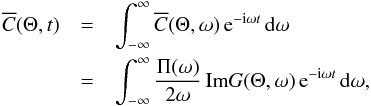$\begin{array}{ccc}\overline{\mathit{C}}\mathrm{\left(}\mathrm{\Theta }\mathit{,t}\mathrm{\right)}& \mathrm{=}& \int \begin{array}{c}\mathrm{\infty }\\ \mathrm{-}\mathrm{\infty }\end{array}\overline{\mathit{C}}\mathrm{\left(}\mathrm{\Theta }\mathit{,\omega }\mathrm{\right)}\hspace{0.17em}{\mathrm{e}}^{\mathrm{-}\mathrm{i}\mathit{\omega t}}\hspace{0.17em}\mathrm{d}\mathit{\omega }\\ & \mathrm{=}& {\mathrm{\int }}_{\mathrm{-}\mathrm{\infty }}^{\mathrm{\infty }}\frac{\mathrm{\Pi }\mathrm{\left(}\mathit{\omega }\mathrm{\right)}}{\mathrm{2}\mathit{\omega }}\hspace{0.17em}\mathrm{Im}\mathit{G}\mathrm{\left(}\mathrm{\Theta }\mathit{,\omega }\mathrm{\right)}\hspace{0.17em}{\mathrm{e}}^{\mathrm{-}\mathrm{i}\mathit{\omega t}}\hspace{0.17em}\mathrm{d}\mathit{\omega ,}\end{array}$(87)where Θ is the angular distance on the surface between the two observation points. The cross-covariance function is also called the time-distance diagram after Duvall et al. (1993). In Fig. 12 we compare the time-distance diagram computed from our power spectrum to an observed time-distance diagram using SOHO/MDI medium degree data (Kosovichev et al. 2000). In order to make this comparison we applied a spatial filter to the simulated power spectrum, F_ℓ = [1−tanh⁽0.03ℓ−3⁾] /2 for ℓ< 100 and 0 otherwise, to remove high-degree modes.

Comparisons of the two time-distance diagrams is encouraging. However, the amplitude of the back-skip ridge at t ~ 250 min is greater in the observations than in the simulations, for which we have no definitive explanation. We think that the most likely explanation is that the damping of the low degree modes is overestimated in our model, resulting in a reduced amplitude of the back-skip branch in the time-distance diagram. Further tuning of the power spectrum is required in order to resolve this discrepancy. For further comparison with the observations, Fig. 13 shows time plots at three different travel distances. The widths and relative amplitudes of the first few skips are in general agreement with the observations.

8. Validation for helioseismology applications

8.1. Convergence of Green’s function

In order to estimate the accuracy of the forward solver, we first measure the convergence of the Green’s function towards a solution G_ref computed for a highly refined mesh (four times more cells) with high-order discretization (order 13). This solution is used as reference since we cannot determine the exact solution to our problem. By choosing a basis of polynomials of order 13 for the finite elements on the refined mesh, the number of degrees of freedom per wavelength is 26 (13 × 2 cells per wavelength), i.e. many more than the 10 points per wavelength used previously.

We compute the Green’s function G^(p) by choosing polynomials of order p in the non-refined mesh containing 10 729 cells. The relative difference between Im G^(p) and Im G_ref, denoted by ε^(p), is plotted in Fig. 14 as a function of the number of degrees of freedom N^(p) = 10729(p + 1)². Explicitly, ${\mathit{\epsilon }}^{\mathrm{\left(}\mathit{p}\mathrm{\right)}}\mathrm{\left(}\mathrm{\Theta }\mathit{,\omega }\mathrm{\right)}\mathrm{=}\frac{\mathrm{|}\mathrm{Im}\hspace{0.17em}{\mathit{G}}^{\mathrm{\left(}\mathit{p}\mathrm{\right)}}\mathrm{(}\mathrm{\Theta }\mathit{,\omega }\mathrm{)}\mathrm{-}\mathrm{Im}\hspace{0.17em}{\mathit{G}}_{\mathrm{ref}}\mathrm{(}\mathrm{\Theta }\mathit{,\omega }\mathrm{\left)}\mathrm{\right|}}{\mathrm{\parallel }\mathrm{Im}\hspace{0.17em}{\mathit{G}}_{\mathrm{ref}}\mathrm{(}\mathrm{·}\mathit{,\omega }\mathrm{)}{\mathrm{\parallel }}_{{\mathit{L}}_{\mathrm{2}}}}\mathrm{·}$(88)In Fig. 14, we plot ε^(p) for different angular distances between the source and the receiver Θ (30°, 60°, and 90°) and different frequencies (3 mHz and 7 mHz). We see that ε^(p) reaches ~10^-5 for orders of discretization p> 10. We obtain a similar convergence when a meridional flow, as described in Appendix B (with surface velocity U = 20 ms^-1), is added to the background.

8.2. Convergence of travel times

Having discussed the accuracy of the Green’s functions at different orders of discretization, we now examine the accuracy of the travel times. Based on Eq. (25), we compute the travel times for waves originating from the pole defined by $\mathit{\delta }{\mathit{\tau }}^{\mathrm{\left(}\mathit{p}\mathrm{\right)}}\mathrm{=}{\mathrm{\int }}_{\mathrm{-}\mathrm{\infty }}^{\mathrm{\infty }}{\mathit{W}}^{\mathrm{\ast }}\mathrm{(}{\mathit{C}}^{\mathrm{\left(}\mathit{p}\mathrm{\right)}}\mathrm{-}{\mathit{C}}_{\mathrm{ref}}\mathrm{)}\hspace{0.17em}\mathrm{d}\mathit{\omega ,}$(89)where C^(p) is the cross-covariance computed from the Green’s functions G^(p) and C_ref is the cross-covariance computed from the G_ref, as defined in the previous section. The Green’s functions were computed for a Nyquist frequency of 8.33 mHz with a frequency resolution of 3.3μHz and a constant damping rate of γ/ 2π = 30 μHz. In Fig. 15, we show that our method achieves a travel-time accuracy of 8 ms for the order of discretization p = 10, with or without the presence of a background meridional flow, as in the previous section. This accuracy could be improved by a factor of 10 if we used polynomials of degree 12; however, the CPU time and memory requirements are increased by 100% and 40%.

8.3. Computational times for the 1.5D, 2.5D and 3D problems

Here we compare the computational times of the 2.5D model with two other models (3D and radial 1.5D). Initially, we examine a simple case of constant sound speed and density spherical layers with the Sommerfeld radiation boundary condition described in Sect. 6.6. This is done in order to demonstrate the computational costs in all three model types. Following this, we compute the computational costs for the more demanding solar cases (1.5D and 2.5D) and neglect the full 3D case because of the high cost. However, we note that computational costs must be multiplied by the number of modes and frequencies required to accurately reconstruct the Green’s function.

Table 2 shows CPU time and memory requirements of the three different models for a single frequency. With each additional dimension, the required memory and CPU time become larger, with a dramatic increase in the full 3D case. A comparison of the model requirements shows that even though the axisymmetric method is more demanding than the radial one, the requirements are not unreasonable for most systems.

9. Travel-time sensitivity kernels

In the results discussed thus far, we have focused on obtaining travel times through the direct modeling of waves propagating in an axisymmetric medium. In this section we address the computation and accuracy of the travel-time kernels outlined in Sect. 4 that describe the spatial sensitivity of travel times to local perturbations in the interior.

9.1. Three-dimensional kernels

Under the “convenient source” assumption, the computation of 3D kernels requires computing four Green’s functions, as explained in Sect. 6. When the medium does not contain a flow, only two Green’s functions are needed. Even in this case, the computational burden is very demanding for a general 3D background (Sect. 8.3). However, it is feasible to compute 3D kernels when the background model is axially or spherically symmetric, under the 2.5D approach outlined thus far.

In the case of spherical symmetry of the background, the kernels can be built from a single Green’s function where the source is located on the pole at the observation height, after a series of rotations. Only the mode m = 0 needs to be computed in this case. This m = 0 Green’s function is then rotated to the desired source location (r₁) and a duplicate is rotated to the receiver location (r₂). The construction of the kernels follows Eqs. (55)–(58).

Figure 16 shows slices through a sound-speed kernel with r₁ at the pole and r₂ at 45° latitude, computed using the rotation of a m = 0 Green’s function and 800 frequencies between 1.5 mHz and 4.5 mHz. In this kernel we see the traditional banana-doughnut shape reported in geophysics (e.g., Marquering et al. 1999) and helioseismology (Birch et al. 2004). For the choice of observable that we have made, the travel-time sensitivity is very small near the ray path (Fig. 16c). Surrounding the ray path are regions of negative and positive sensitivities corresponding to the consecutive Fresnel zones. The values near the surface are not numerical noise but are due to high spatial frequencies. Figure 16 is a 3D illustration of the sound-speed kernel and also shows the values on the sphere at radius r = 0.95 R_⊙. The sensitivity is maximum near the surface around the two observation points. We note that we have plotted the product cK_c to better render the deeper layers. The computation of the m = 0 Green’s function took approximately 1 h using 200 cores. The post-processing consists mostly in computing the rotated Green’s functions and took approximately 3 h.

9.2. Longitudinally averaged kernels

For an axisymmetric (but not necessary spherically symmetric) background, the Green’s functions must be constructed by summing a sufficient number of m modes. Here, in addition, we only consider axisymmetric perturbations, q_α = q_α(r,θ), and we wish to determine the 2D spatial sensitivity of the travel times by averaging the kernels over longitude. Useful applications include rotation (u_φ) and meridional circulation (u_θ). For axisymmetric perturbations, we have $\mathit{\delta \tau }\mathrm{\left(}{r}\mathrm{1}\mathit{,}{r}\mathrm{2}\mathrm{\right)}\mathrm{=}\mathrm{2}\mathit{\pi }\sum _{\mathit{\alpha }}{\mathrm{\int }}_{\mathrm{0}}^{\mathit{\pi }}\mathrm{d}\mathit{\theta }{\mathrm{\int }}_{\mathrm{0}}^{\mathit{R}}\mathrm{d}\mathit{r\delta }{\mathit{q}}_{\mathit{\alpha }}\mathrm{\left(}\mathit{r,\theta }\mathrm{\right)}\mathrm{⟨}{\mathit{K}}_{\mathit{\alpha }}\mathrm{⟩}\mathrm{\left(}\mathit{r,\theta }\mathrm{;}{r}\mathrm{1}\mathit{,}{r}\mathrm{2}\mathrm{\right)}$(90)where ⟨ K_α ⟩ is the longitudinally averaged kernel $\mathrm{⟨}{\mathit{K}}_{\mathit{\alpha }}\mathrm{⟩}\mathrm{\left(}\mathit{r,\theta }\mathrm{;}{r}\mathrm{1}\mathit{,}{r}\mathrm{2}\mathrm{\right)}\mathrm{=}\frac{{\mathit{r}}^{\mathrm{2}}\sin \mathit{\theta }}{\mathrm{2}\mathit{\pi }}{\mathrm{\int }}_{\mathrm{0}}^{\mathrm{2}\mathit{\pi }}{\mathit{K}}_{\mathit{\alpha }}\mathrm{\left(}\mathit{r,\theta ,\phi }\mathrm{;}{r}\mathrm{1}\mathit{,}{r}\mathrm{2}\mathrm{\right)}\hspace{0.17em}\mathrm{d}\mathit{\phi }\mathit{.}$(91)Let us define the Green’s function and the cross-covariance function in terms of their longitudinal mode components G^m and C^m as follows: $\begin{array}{ccc}& & \mathit{G}\mathrm{\left(}{r}\mathit{,}{r}\mathrm{1}\mathit{,\omega }\mathrm{\right)}\mathrm{=}\sum _{\mathit{m}\mathrm{=}\mathrm{-}\mathrm{\infty }}^{\mathrm{\infty }}{\mathit{G}}^{\mathit{m}}\mathrm{\left(}\begin{array}{c}\mathrm{˜}\\ {r}\end{array}\mathit{,}{\begin{array}{c}\mathrm{˜}\\ {r}\end{array}}_{\mathrm{1}}\mathit{,\omega }\mathrm{\right)}\hspace{0.17em}{\mathrm{e}}^{\mathrm{i}\mathit{m}\mathrm{(}\mathit{\phi }\mathrm{-}{\mathit{\phi }}_{\mathrm{1}}\mathrm{)}}\mathit{,}\\ & & \overline{\mathit{C}}\mathrm{\left(}{r}\mathrm{1}\mathit{,}{r}\mathit{,\omega }\mathrm{\right)}\mathrm{=}\sum _{\mathit{m}\mathrm{=}\mathrm{-}\mathrm{\infty }}^{\mathrm{\infty }}{\mathit{C}}^{\mathit{m}}\mathrm{\left(}{\begin{array}{c}\mathrm{˜}\\ {r}\end{array}}_{\mathrm{1}}\mathit{,}\begin{array}{c}\mathrm{˜}\\ {r}\end{array}\mathit{,\omega }\mathrm{\right)}\hspace{0.17em}{\mathrm{e}}^{\mathrm{i}\mathit{m}\mathrm{(}\mathit{\phi }\mathrm{-}{\mathit{\phi }}_{\mathrm{1}}\mathrm{)}}\mathit{.}\end{array}$(92)It is important to note the order of the variables in G and $\overline{\mathit{C}}$ in the above notations. Using the formulation of the kernels given by Eq. (43), we obtain $\begin{array}{ccc}& & {\mathit{K}}_{\mathit{\alpha }}\mathrm{\left(}\mathit{r,\theta ,\phi }\mathrm{;}{r}\mathrm{1}\mathit{,}{r}\mathrm{2}\mathrm{\right)}\mathrm{=}\\ & & \mathrm{-}{\mathrm{\int }}_{\mathrm{-}\mathrm{\infty }}^{\mathrm{\infty }}\mathrm{d}\mathit{\omega }{\mathit{W}}^{\mathrm{\ast }}\sum _{\mathit{m,}{\mathit{m}}^{\mathrm{\prime }}}{\mathrm{ℒ}}_{\mathit{\alpha }}\mathrm{[}{\mathit{G}}^{\mathit{m}}\mathrm{\left(}{\begin{array}{c}\mathrm{˜}\\ {r}\end{array}}_{\mathrm{2}}\mathit{,}\begin{array}{c}\mathrm{˜}\\ {r}\end{array}\mathrm{\right)}{\mathrm{e}}^{\mathrm{i}\mathit{m}\mathrm{(}{\mathit{\phi }}_{\mathrm{2}}\mathrm{-}\mathit{\phi }\mathrm{)}}\mathit{,}{\mathit{C}}^{{\mathit{m}}^{\mathrm{\prime }}}\mathrm{\left(}{\begin{array}{c}\mathrm{˜}\\ {r}\end{array}}_{\mathrm{1}}\mathit{,}\begin{array}{c}\mathrm{˜}\\ {r}\end{array}\mathrm{\right)}{\mathrm{e}}^{\mathrm{-}\mathrm{i}{\mathit{m}}^{\mathrm{\prime }}\mathrm{(}{\mathit{\phi }}_{\mathrm{1}}\mathrm{-}\mathit{\phi }\mathrm{)}}\mathrm{]}\\ & & \mathrm{-}{\mathrm{\int }}_{\mathrm{-}\mathrm{\infty }}^{\mathrm{\infty }}\mathrm{d}\mathit{\omega }{\mathit{W}}^{\mathrm{\ast }}\sum _{\mathit{m,}{\mathit{m}}^{\mathrm{\prime }}}{\mathrm{ℒ}}_{\mathit{\alpha }}^{\mathrm{\ast }}\mathrm{[}{\mathit{G}}^{\mathit{m}\mathrm{\ast }}\mathrm{\left(}{\begin{array}{c}\mathrm{˜}\\ {r}\end{array}}_{\mathrm{1}}\mathit{,}\begin{array}{c}\mathrm{˜}\\ {r}\end{array}\mathrm{\right)}{\mathrm{e}}^{\mathrm{-}\mathrm{i}\mathit{m}\mathrm{(}{\mathit{\phi }}_{\mathrm{1}}\mathrm{-}\mathit{\phi }\mathrm{)}}\mathit{,}{\mathit{C}}^{{\mathit{m}}^{\mathrm{\prime }}\mathrm{\ast }}\mathrm{\left(}{\begin{array}{c}\mathrm{˜}\\ {r}\end{array}}_{\mathrm{2}}\mathit{,}\begin{array}{c}\mathrm{˜}\\ {r}\end{array}\mathrm{\right)}{\mathrm{e}}^{\mathrm{i}{\mathit{m}}^{\mathrm{\prime }}\mathrm{(}{\mathit{\phi }}_{\mathrm{2}}\mathrm{-}\mathit{\phi }\mathrm{)}}\mathrm{]}\mathit{.}\end{array}$(93)Using the explicit expressions for the bilinear operators ℒ_α (Eqs. (55)-(58)), we can then obtain the longitudinally averaged kernels for all perturbations q_α.

As an example, the flow kernels can be written as a sum $\mathrm{⟨}{\mathit{K}}_{{\mathit{u}}_{\mathit{k}}}\mathrm{⟩}\mathrm{\left(}\mathit{r,\theta }\mathrm{;}{r}\mathrm{1}\mathit{,}{r}\mathrm{2}\mathrm{\right)}\mathrm{=}\sum _{\mathit{m}\mathrm{=}\mathrm{-}\mathrm{\infty }}^{\mathrm{\infty }}\mathrm{⟨}{\mathit{K}}_{{\mathit{u}}_{\mathit{k}}}{\mathrm{⟩}}^{\mathit{m}}\mathrm{\left(}\mathit{r,\theta }\mathrm{;}{r}\mathrm{1}\mathit{,}{r}\mathrm{2}\mathrm{\right)}$(94)over azimuthal components: $\begin{array}{ccc}\mathrm{⟨}{\mathit{K}}_{{\mathit{u}}_{\mathit{k}}}{\mathrm{⟩}}^{\mathit{m}}& \mathrm{=}& \mathrm{2}\mathrm{i}\mathit{\rho }{\mathit{r}}^{\mathrm{2}}\sin \mathit{\theta }{\mathrm{\int }}_{\mathrm{-}\mathrm{\infty }}^{\mathrm{\infty }}\mathrm{d}\mathit{\omega }\hspace{0.17em}\mathit{\omega }{\mathit{W}}^{\mathrm{\ast }}{\mathrm{e}}^{\mathrm{i}\mathit{m}\mathrm{(}{\mathit{\phi }}_{\mathrm{2}}\mathrm{-}{\mathit{\phi }}_{\mathrm{1}}\mathrm{)}}\\ & & \mathrm{\times }\mathrm{[}{\mathit{G}}^{\mathit{m}}\mathrm{\left(}{\begin{array}{c}\mathrm{˜}\\ {r}\end{array}}_{\mathrm{2}}\mathit{,}\begin{array}{c}\mathrm{˜}\\ {r}\end{array}\mathrm{\right)}\hspace{0.17em}\begin{array}{c}\mathrm{˜}\\ {\mathit{\partial }}_{\mathit{k}}\end{array}{\mathit{C}}^{\mathrm{-}\mathit{m}}\mathrm{\left(}{\begin{array}{c}\mathrm{˜}\\ {r}\end{array}}_{\mathrm{1}}\mathit{,}\begin{array}{c}\mathrm{˜}\\ {r}\end{array}\mathrm{\right)}\mathrm{-}{\mathit{G}}^{\mathit{m}\mathrm{\ast }}\mathrm{\left(}{\begin{array}{c}\mathrm{˜}\\ {r}\end{array}}_{\mathrm{1}}\mathit{,}\begin{array}{c}\mathrm{˜}\\ {r}\end{array}\mathrm{\right)}\hspace{0.17em}\begin{array}{c}\mathrm{˜}\\ {\mathit{\partial }}_{\mathit{k}}\end{array}{\mathit{C}}^{\mathrm{-}\mathit{m}\mathrm{\ast }}\mathrm{(}{\begin{array}{c}\mathrm{˜}\\ {r}\end{array}}_{\mathrm{2}}\mathit{,}\begin{array}{c}\mathrm{˜}\\ {r}\end{array}{\mathrm{)}}^{\mathrm{]}}\mathit{,}\end{array}$(95)where the operator $\begin{array}{c}{\mathrm{˜}}_{}\\ {\mathit{\partial }}_{\mathit{k}}\end{array}$ is either $\begin{array}{c}{}_{\mathrm{˜}}\\ {\mathit{\partial }}_{\mathit{r}}\end{array}\mathrm{=}{\mathit{\partial }}_{\mathit{r}}$, $\begin{array}{c}{}_{\mathrm{˜}}\\ {\mathit{\partial }}_{\mathit{\theta }}\end{array}\mathrm{=}{\mathit{\partial }}_{\mathit{\theta }}\mathit{/}\mathit{r}$, or $\begin{array}{c}{}_{\mathrm{˜}}\\ {\mathit{\partial }}_{\mathit{\phi }}\end{array}\mathrm{=}\mathrm{i}\mathit{m}\mathit{/}\mathrm{\left(}\mathit{r}\sin \mathit{\theta }\mathrm{\right)}$.

In practice, ${\mathit{G}}^{\mathit{m}}\mathrm{\left(}{\begin{array}{c}{}_{\mathrm{˜}}\\ {r}\end{array}}_{\mathit{j}}\mathit{,}\begin{array}{c}{}_{\mathrm{˜}}\\ {r}\end{array}\mathit{,\omega }\mathrm{\right)}$ is obtained using generalized seismic reciprocity, ${\mathit{G}}^{\mathit{m}}\mathrm{\left(}{\begin{array}{c}{}_{\mathrm{˜}}\\ {r}\end{array}}_{\mathit{j}}\mathit{,}\begin{array}{c}{}_{\mathrm{˜}}\\ {r}\end{array}\mathit{,\omega }\mathrm{\right)}\mathrm{=}{\mathit{G}}^{\mathrm{-}\mathit{m}}\mathrm{(}\begin{array}{c}{}_{\mathrm{˜}}\\ {r}\end{array}\mathit{,}{\begin{array}{c}{}_{\mathrm{˜}}\\ {r}\end{array}}_{\mathit{j}}\mathit{,\omega }\mathrm{;}\mathrm{-}{u}\mathrm{)}$, performing a simulation with a source at ${\begin{array}{c}{\mathrm{˜}}_{}\\ {r}\end{array}}_{\mathit{j}}$. Using the convenient source of excitation, the cross-covariance is linked to the Green’s function by Eq. (49). It is possible to obtain a similar relation for the Fourier coefficients: ${\mathit{C}}^{\mathit{m}}\mathrm{\left(}{\begin{array}{c}\mathrm{˜}\\ {r}\end{array}}_{\mathrm{1}}\mathit{,}\begin{array}{c}\mathrm{˜}\\ {r}\end{array}\mathit{,\omega }\mathrm{\right)}\mathrm{=}\frac{\mathrm{\Pi }\mathrm{\left(}\mathit{\omega }\mathrm{\right)}}{\mathrm{4}\mathrm{i}\mathit{\omega }}\left[{\mathit{G}}^{\mathit{m}}\mathrm{\left(}\begin{array}{c}\mathrm{˜}\\ {r}\end{array}\mathit{,}{\begin{array}{c}\mathrm{˜}\\ {r}\end{array}}_{\mathrm{1}}\mathit{,\omega }\mathrm{\right)}\mathrm{-}{\mathit{G}}^{\mathrm{-}\mathit{m}\mathrm{\ast }}\mathrm{(}\begin{array}{c}\mathrm{˜}\\ {r}\end{array}\mathit{,}{\begin{array}{c}\mathrm{˜}\\ {r}\end{array}}_{\mathrm{1}}\mathit{,\omega }\mathrm{;}\mathrm{-}{u}\mathrm{)}\right]\mathit{.}$(96)This means that the (3D) kernels can be computed using only the azimuthal modes of the Green’s function obtained from the 2.5D solver.

Several comments can be made:

• If one of the observation points is on the rotation axis, then only the m = 0mode of the Green’s function is required. For a measurementbetween two arbitrary points at the surface of the Sun, thecomputation of many modes is required (see next section).

• If the background model contains a flow, then the Green’s function for a reversed flow is also required in order to compute the cross-covariance as shown by Eq. (96).

• In the case of no background flow, Eq. (66)shows that only the m ≥ 0 solutions need to be computed since G^{− m} = G^m.

• If the kernels for points (θ₁,φ₁) and (θ₂,φ₂) have been computed, then we obtain for free the kernels for points with different longitudes since the only term in Eq. (95)that depends on the longitudes is the exponential e^{im(φ₂−φ₁)}.

9.3. Accuracy of travel-time kernels for flows

Consider a spherically symmetric background reference model with no flow. Figure 17 shows the flow kernels ⟨ K_ur ⟩ = ⟨ K_ur ⟩ ^{m = 0} and ⟨ K_uθ ⟩ = ⟨ K_uθ ⟩ ^{m = 0} with a point r₁ on the pole (at the solar surface) and a point r₂ located at latitude 45°. The kernel ⟨ K_uφ ⟩ ^{m = 0} is zero by construction because ⟨ K_uφ ⟩ ^m is proportional to m. The 2D kernels for u_r and u_θ display Fresnel zones as do the 3D kernels, however, the null points along the ray path are absent here because of integration in the longitudinal direction.Additionally, as reported by Birch & Gizon (2007), the kernels exhibit hyperbola-like patterns near point r₁. This pattern is due to scattering from distant sources (Gizon & Birch 2002) and is not present in Earth seismology kernels for point-source earthquakes. We refer the reader to the work by Duvall et al. (2006) for an observational study of 2D horizontal sensitivity kernels. The right-hand panel of Fig. 17 compares the travel times computed in two different ways to evaluate the accuracy of the kernels: (1) by multiplying the kernels by a flow model u and integrating (Eq. (90)) and (2) by computing the difference δC = C(u)−C(u = 0) and then measuring the travel time (Eq. (25)). Here we have used the meridional flow model shown in Appendix B with a maximum flow speed of 20 ms^-1 at the surface. For the comparison we have considered three separation distances (30°, 45°, and 60°) and the two directions, δτ(r₁,r₂) and δτ(r₂,r₁). The kernel-based computation of the travel times and the direct computation agree to within 10^-3 s. This is an important result as it demonstrates that our kernels have sufficient accuracy for the interpretation of solar travel times. For meridional circulation measurements, the noise in the travel times is typically in the range 0.1–0.5 s, found by averaging data over four years (Rajaguru & Antia 2015).

For practical applications, the two points should be off-axis since helioseismic observations are limited to a center-to-limb distance of ~70°. In such cases the azimuthally averaged kernels require the computation of many components ⟨ K ⟩ ^m. Figure 18 shows the components of flow kernel computed from Eq. (95)for all m ≤ 35. In this figure the travel times are measured between points at latitudes 61° and 19°, both along the central meridian. With this separation distance of 42° the ray path reaches a depth of 0.72 R_⊙. Like before, the kernels are not symmetric about the center point between the observation points and have features similar those seen in Fig. 17.

To test the convergence of these kernels, we calculate individual kernels including all modes | m | ≤ m_max and compute travel times as a function of m_max in the presence of the same meridional flow as used previously. The right-hand panel of Fig. 18 shows that the travel times converge to an asymptotic value for m_max> 25 with an accuracy of ~0.01 s. We note that a larger m_max is needed to achieve convergence for shorter separation distances.

9.4. Filtering

Filtering the observations in the ℓ-ω domain is common practice in helioseismology. Several choices of filters have been proposed: filters in ω space, phase-speed filters, and ridge filters (see, e.g., Gizon & Birch 2005). To interpret any particular travel-time measurement, the sensitivity kernels must account for the proper frequency content of the seismic data set by the filtering. This dependency of the kernel on the filter has been studied previously (e.g., Birch et al. 2004; Böning et al. 2016).

Symbolically, the filtered observation, Ψ, is obtained by applying a filtering operator, F, to the original wavefield, ψ: $\mathrm{\Psi }\mathrm{\left(}{r}\mathit{,\omega }\mathrm{\right)}\mathrm{=}F\mathrm{\left[}\mathit{\psi }\mathrm{\right(}{r}\mathit{,\omega }\mathrm{\left)}\mathrm{\right]}\mathit{.}$(97)The corresponding kernel is obtained by applying the filtering operator twice to the original kernel: $\begin{array}{ccc}{K}_{\mathit{\alpha }}\mathrm{\left(}{r}\mathit{,}{r}\mathrm{1}\mathit{,}{r}\mathrm{2}\mathrm{\right)}& \mathrm{=}& \mathrm{-}{\mathrm{\int }}_{\mathrm{-}\mathrm{\infty }}^{\mathrm{\infty }}{\mathit{W}}^{\mathrm{\ast }}{\mathrm{ℒ}}_{\mathit{\alpha }}\left[G\mathrm{\left(}{r}\mathrm{2}\mathit{,}{r}\mathit{,\omega }\mathrm{\right)}\mathit{,}C\mathrm{\left(}{r}\mathrm{1}\mathit{,}{r}\mathit{,\omega }\mathrm{\right)}\right]\mathrm{d}\mathit{\omega }\\ & & \mathrm{-}{\mathrm{\int }}_{\mathrm{-}\mathrm{\infty }}^{\mathrm{\infty }}{\mathit{W}}^{\mathrm{\ast }}{\mathrm{ℒ}}_{\mathit{\alpha }}^{\mathrm{\ast }}\left[G^{\mathrm{\ast }}\mathrm{\left(}{r}\mathrm{1}\mathit{,}{r}\mathit{,\omega }\mathrm{\right)}\mathit{,}{C}^{\mathrm{\ast }}\mathrm{\left(}{r}\mathrm{2}\mathit{,}{r}\mathit{,\omega }\mathrm{\right)}\right]\mathrm{d}\mathit{\omega ,}\\ & & \end{array}$(98)where the filtered Green’s function and cross-covariance are $\begin{array}{ccc}G\mathrm{\left(}{r}\mathrm{1}\mathit{,}{r}\mathit{,\omega }\mathrm{\right)}& \mathrm{=}& F_{\mathrm{1}}\mathrm{\left[}\mathit{G}\mathrm{\right(}{r}\mathrm{1}\mathit{,}{r}\mathit{,\omega }\mathrm{\left)}\mathrm{\right]}\mathit{,}\\ C\mathrm{\left(}{r}\mathrm{1}\mathit{,}{r}\mathit{,\omega }\mathrm{\right)}& \mathrm{=}& F_{\mathrm{1}}\mathrm{\left[}\overline{\mathit{C}}\mathrm{\right(}{r}\mathrm{1}\mathit{,}{r}\mathit{,\omega }\mathrm{\left)}\mathrm{\right]}\\ & \mathrm{=}& \frac{\mathrm{\Pi }\mathrm{\left(}\mathit{\omega }\mathrm{\right)}}{\mathrm{4}\mathrm{i}\mathit{\omega }}\left[G\mathrm{(}{r}\mathrm{1}\mathit{,}{r}\mathit{,\omega }\mathrm{;}\mathrm{-}{u}\mathrm{)}\mathrm{-}{G}^{\mathrm{\ast }}\mathrm{\left(}{r}\mathrm{1}\mathit{,}{r}\mathit{,\omega }\mathrm{\right)}\right]\mathit{,}\end{array}$and the W function is computed with the choice C_ref =C. Here, F₁ indicates that the filtering has to be done with respect to the point r₁.

The filtered Green’s function may be obtained by filtering the delta source function. To see this, we use generalized seismic reciprocity $\begin{array}{ccc}G\mathrm{\left(}{r}\mathrm{1}\mathit{,}{r}\mathit{,\omega }\mathrm{\right)}& \mathrm{=}& F_{\mathrm{1}}\mathrm{\left[}\mathit{G}\mathrm{\right(}{r}\mathit{,}{r}\mathrm{1}\mathit{,\omega }\mathrm{;}\mathrm{-}{u}\mathrm{\left)}\mathrm{\right]}\\ & \mathrm{=}& {\mathrm{\int }}_{\mathit{V}}\mathit{G}\mathrm{(}{r}\mathit{,}{r}\mathrm{\prime }\mathit{,\omega }\mathrm{;}\mathrm{-}{u}\mathrm{)}\hspace{0.17em}{F}_{\mathrm{1}}\mathrm{\left[}\mathit{\delta }\mathrm{\right(}{r}\mathrm{1}\mathrm{-}{r}\mathrm{\prime }\mathrm{\left)}\mathrm{\right]}\hspace{0.17em}\mathrm{d}{r}\mathrm{\prime }\mathit{,}\end{array}$(101)where $\begin{array}{ccc}{\mathrm{ℱ}}_{\mathrm{1}}\mathrm{\left[}\mathit{\delta }\mathrm{\right(}{r}\mathrm{1}\mathrm{-}{r}\mathrm{\prime }\mathrm{\left)}\mathrm{\right]}& \mathrm{=}& \mathit{\delta }\mathrm{(}{\mathit{r}}_{\mathrm{1}}\mathrm{-}{\mathit{r}}^{\mathrm{\prime }}\mathrm{)}{F}_{\mathrm{1}}\left[\sum _{\mathit{\ell }\mathrm{=}\mathrm{0}}^{\mathrm{\infty }}\sum _{\mathit{m}\mathrm{=}\mathrm{-}\mathit{\ell }}^{\mathit{\ell }}{\mathit{Y}}_{\mathit{\ell }}^{\mathit{m}}\mathrm{\left(}{r̂}\mathrm{1}\mathrm{\right)}{\mathit{Y}}_{\mathit{\ell }}^{\mathit{m}\mathrm{\ast }}\mathrm{\left(}{r̂}\mathrm{\prime }\mathrm{\right)}\right]\\ & \mathrm{=}& \end{array}$(102)is the filtered delta function source. In the above expression F_ℓ(ω) can be either a phase-speed filter or a ridge filter. We note that the filtered source function is a function of frequency.

If the background is spherically symmetric with no background flow, it is also possible to compute the non-filtered Green’s function and to perform the filtering a posteriori. In this case, the Green’s function G(r₁,r,ω) depends only on the depths r₁ and r and on the angular distance Θ₁ between the two points $\mathit{G}\mathrm{\left(}{r}\mathrm{1}\mathit{,}{r}\mathit{,\omega }\mathrm{\right)}\mathrm{=}\mathit{G}\mathrm{\left(}{\mathit{r}}_{\mathrm{1}}\mathit{,r,}{\mathrm{\Theta }}_{\mathrm{1}}\mathit{,\omega }\mathrm{\right)}\mathit{,}$(103)where . The filtered Green’s function takes the form $\begin{array}{ccc}\hspace{0.17em}\begin{array}{c}\begin{array}{c}\end{array}G\mathrm{\left(}{r}\mathrm{1}\mathit{,}{r}\mathit{,\omega }\mathrm{\right)}\mathrm{=}\sum _{\mathit{\ell }\mathrm{=}\mathrm{-}\mathrm{\infty }}^{\mathrm{\infty }}{\mathit{F}}_{\mathit{\ell }}\mathrm{\left(}\mathit{\omega }\mathrm{\right)}{\mathit{G}}_{\mathit{\ell }}\mathrm{\left(}{\mathit{r}}_{\mathrm{1}}\mathit{,r,\omega }\mathrm{\right)}{\mathit{P}}_{\mathit{\ell }}\mathrm{\left(}\cos {\mathrm{\Theta }}_{\mathrm{1}}\mathrm{\right)}\mathit{,}\end{array}& & \end{array}$(104)where ${\mathit{G}}_{\mathit{\ell }}\mathrm{\left(}{\mathit{r}}_{\mathrm{1}}\mathit{,r,\omega }\mathrm{\right)}\mathrm{=}\frac{\mathrm{2}\mathit{\ell }\mathrm{+}\mathrm{1}}{\mathrm{2}}{\mathrm{\int }}_{\mathrm{0}}^{\mathit{\pi }}\mathit{G}\mathrm{\left(}{\mathit{r}}_{\mathrm{1}}\mathit{,r,}\mathrm{\Theta }\mathit{,\omega }\mathrm{\right)}{\mathit{P}}_{\mathit{\ell }}\mathrm{\left(}\cos \mathrm{\Theta }\mathrm{\right)}\sin \mathrm{\Theta }\hspace{0.17em}\mathrm{d\Theta }$(105)is the projection of G on the Legendre polynomials. Using seismic reciprocity we obtain G_ℓ(r₁,r,ω) = G_ℓ(r,r₁,ω), and Eq. (104) implies $G\mathrm{\left(}{r}\mathrm{1}\mathit{,}{r}\mathit{,\omega }\mathrm{\right)}\mathrm{=}G\mathrm{\left(}{r}\mathit{,}{r}\mathrm{1}\mathit{,\omega }\mathrm{\right)}\mathit{.}$(106)Thus, if the background is spherically symmetric, we also have seismic reciprocity for the filtered Green’s function: the filtering can be seen as a post-processing operation on r at fixed source position r₁. Otherwise, a filtered source should be used, as given by Eq. (102).

As a special case, we computed the azimuthally averaged kernels of Eq. (95)for filtered observations when r₁ is located at the pole and u = 0. As mentioned previously, only the m = 0 component of the Green’s function is needed. Figure 19 shows the effect of applying a phase-speed filter to the kernel ⟨ K_uθ ⟩ with r₁ at the pole and r₂ at a co-latitude of 15.36°. The phase-speed filter is centered at 125.2 km s^-1 with a width of 12.3 km s^-1. These values were chosen to be the same as for filter #11 in Duvall & Hanasoge (2013). Once the filter is applied the sensitivity to u_θ is predominantly near the base of the ray path. This filtered kernel appears to be similar to the K₆ case from Böning et al. (2016) indicating general agreement with their work.

10. Conclusion

We have presented a new framework for computational helioseismology by solving the forward problem in the frequency domain. For the sake of simplicity, we considered a simplified scalar acoustic wave equation and assumed spatially uncorrelated sources of excitation distributed through the Sun. Under such conditions, the cross-covariance can be obtained directly from the imaginary part of the frequency-domain Green’s function. This leads to a convenient, flexible, and fast way to compute accurate kernels. The analytical work involved in this framework is less cumbersome than previous work that relies on normal-mode expansions of the kernels (e.g., Birch & Gizon 2007; Burston et al. 2015; Böning et al. 2016). The framework can be extended to the vectorial wave equation quite easily using existing Montjoie vectorial setups (e.g. Péron et al. 2016, for Maxwell’s equations). The scalar equation captures the propagation of acoustic waves through a solar-like medium and leads to an oscillation power spectrum that compares well with observations. The present setup will be very useful to test new methods, including instrumental and projection effects, but also to interpret existing travel-time measurements for rotation, meridional circulation, and axisymmetric structures like the average supergranule.

In future work we intend to address the inverse problem. Specifically, we wish to find the parameters δq of the background model (sound speed, density, flows) such that the travel times τ from the model are consistent with the observed travel times τ_obs. This is generally done by solving a linear system of the form δτ = K δq + n, where K is a matrix of kernels and n is a vector of travel-time noises, defined through the noise covariance matrix Λ = E [nn^T] (see Gizon & Birch 2004; Fournier et al. 2014). This problem can be solved by classical regularization methods such as regularized least square (RLS; e.g., Kosovichev 1996) or optimally localized averaging (OLA, e.g., Haber et al. 2004). Another approach is to solve a non-linear inverse problem defined in terms of the partial differential equation. Different methods exist such as the Landweber iteration (Hanke et al. 1995) and Newton-type methods such as the iteratively regularized Gauss-Newton (Bakushinskii 1992) or Newton conjugate gradient methods (Hanke 1997). Most of these methods avoid the explicit computation of sensitivity kernels. All these inverse methods are feasible under the assumption of an axisymmetric background model, thanks to the embarrassingly parallel workload in m and ω. The last iteration of the inversion produces a 3D model of the solar internal properties. Using a full 3D forward solver is currently not practical.

---

Acknowledgments

L.G. and A.C.B. developed the general theoretical framework. H.B., J.C., and M.D. developed tools to solve the wave equation (Montjoie package). C.S.H., M.L., and D.F. implemented the tools in the solar context, tuned the power spectrum, and computed the kernels. All authors contributed to the writing of the paper. L.G. acknowledges generous financial support from the State of Lower Saxony, Germany, and partial support from the Center for Space Science at the NYU Abu Dhabi Institute, UAE, under grant G1502. The computer infrastructure was provided in part by the German Data Center for SDO funded by the German Aerospace Center (DLR). The research leading to these results has received funding from the EU FP7/2007-2013 program under grant agreement No. 312844 (SpaceInn). The Global Oscillation Network Group is funded by the National Science Foundation. The HMI project is supported by NASA contract NAS5-02139. Part of the numerical experiments presented in this paper were carried out using the PLAFRIM experimental testbed, developed under the Inria PlaFRIM development action with support from Bordeaux INP, LABRI, IMB, Conseil régional d’Aquitaine, Université de Bordeaux, CNRS, and ANR (Programme des investissements d’avenir).

References

Appendix A: Solving the eigenvalue problem using ADIPLS

We modified ADIPLS to solve the eigenvalue problem $\mathrm{\mathscr{H}}\mathrm{\left[}{\xi }\mathrm{\right]}\mathrm{=}{\mathit{\omega }}^{\mathrm{2}}{\xi }$(A.1)where ℋ is given by Eq. (2) and we neglected the gravity terms. Using the same notation as the one used by Christensen-Dalsgaard (2008), the corresponding eigenvalue problem for the eigenfrequency and the eigenfunction of a mode takes the form $\begin{array}{ccc}{\mathit{\omega }}^{\mathrm{2}}{\mathit{\xi }}_{\mathit{r}}& \mathrm{=}& \mathrm{-}\frac{\mathrm{1}}{\mathit{\rho }}\frac{\mathrm{d}}{\mathrm{d}\mathit{r}}\left[\mathit{\rho }{\mathit{c}}^{\mathrm{2}}\left(\frac{\mathrm{d}{\mathit{\xi }}_{\mathit{r}}}{\mathrm{d}\mathit{r}}\mathrm{+}\mathrm{2}\frac{{\mathit{\xi }}_{\mathit{r}}}{\mathit{r}}\mathrm{-}{\mathit{L}}^{\mathrm{2}}\frac{{\mathit{\xi }}_{\mathit{h}}}{\mathit{r}}\right)\right]\mathit{,}\\ {\mathit{\omega }}^{\mathrm{2}}{\mathit{\xi }}_{\mathit{h}}& \mathrm{=}& \mathrm{-}{\mathit{c}}^{\mathrm{2}}\left(\frac{\mathrm{1}}{\mathit{r}}\frac{\mathrm{d}{\mathit{\xi }}_{\mathit{r}}}{\mathrm{d}\mathit{r}}\mathrm{+}\mathrm{2}\frac{{\mathit{\xi }}_{\mathit{r}}}{{\mathit{r}}^{\mathrm{2}}}\mathrm{-}{\mathit{L}}^{\mathrm{2}}\frac{{\mathit{\xi }}_{\mathit{h}}}{{\mathit{r}}^{\mathrm{2}}}\right)\mathit{,}\end{array}$where L² = ℓ(ℓ + 1), and ξ_r(r) and ξ_h(r) are the radial and horizontal eigenfunctions. The equations can be rewritten as $\begin{array}{ccc}\mathit{r}\frac{\mathrm{d}{\mathit{\xi }}_{\mathit{r}}}{\mathrm{d}\mathit{r}}& \mathrm{=}& \mathrm{-}\mathrm{2}{\mathit{\xi }}_{\mathit{r}}\mathrm{+}\left({\mathit{L}}^{\mathrm{2}}\mathrm{-}\frac{{\mathit{\omega }}^{\mathrm{2}}{\mathit{r}}^{\mathrm{2}}}{{\mathit{c}}^{\mathrm{2}}}\right){\mathit{\xi }}_{\mathit{h}}\mathit{,}\\ \mathit{r}\frac{\mathrm{d}{\mathit{\xi }}_{\mathit{h}}}{\mathrm{d}\mathit{r}}& \mathrm{=}& {\mathit{\xi }}_{\mathit{r}}\mathrm{-}\left(\mathrm{1}\mathrm{+}\frac{\mathrm{d}\ln \mathit{\rho }}{\mathrm{d}\ln \mathit{r}}\right){\mathit{\xi }}_{\mathit{h}}\mathit{,}\end{array}$which, in ADIPLS adimensionalized form (see Christensen-Dalsgaard 2008), become $\begin{array}{ccc}\mathit{x}\frac{\mathrm{d}{\mathit{y}}_{\mathrm{1}}}{\mathrm{d}\mathit{x}}& \mathrm{=}& \mathrm{-}\mathrm{2}{\mathit{y}}_{\mathrm{1}}\mathrm{+}\left(\mathrm{1}\mathrm{-}\frac{{\mathit{V}}_{\mathit{g}}}{\mathit{\eta }}\right){\mathit{y}}_{\mathrm{2}}\mathit{,}\\ \mathit{x}\frac{\mathrm{d}{\mathit{y}}_{\mathrm{2}}}{\mathrm{d}\mathit{x}}& \mathrm{=}& {\mathit{L}}^{\mathrm{2}}{\mathit{y}}_{\mathrm{1}}\mathrm{+}\mathrm{(}\mathit{A}\mathrm{+}{\mathit{V}}_{\mathit{g}}\mathrm{-}{\mathrm{1}}^{\mathrm{)}}{\mathit{y}}_{\mathrm{2}}\mathit{.}\end{array}$We modified ADIPLS, by changing the file rhs.n.d.f in such a way that it solves Eqs. (A.6) and (A.7), with a free surface boundary condition.

We calculated the frequency splittings in presence of differential rotation by evaluating the integral $\mathit{\delta }{\mathit{\omega }}_{\mathit{n\ell m}}\mathrm{=}\mathit{m}{\mathrm{\int }}_{\mathrm{0}}^{\mathit{R}}\mathrm{d}\mathit{r}{\mathrm{\int }}_{\mathrm{0}}^{\mathit{\pi }}{\mathit{K}}_{\mathit{n\ell m}}\mathrm{\left(}\mathit{r,\theta }\mathrm{\right)}\mathrm{\Omega }\mathrm{\left(}\mathit{r,\theta }\mathrm{\right)}\hspace{0.17em}\mathit{r}\mathrm{d}\mathit{\theta }$(A.8)where the rotation profile Ω(r,θ) is defined by Eq. (86), and K_nℓm(r,θ) are the rotational sensitivity kernels (see Chap. 8.4 in Christensen-Dalsgaard 2003), which depend on ξ_r and ξ_h.

Appendix B: Meridional flow model

Various models of meridional flow cells can be found in the literature (e.g., van Ballegooijen & Choudhuri 1988; Dikpati & Choudhuri 1995; Jouve et al. 2008). In these models the flow is expressed through a stream function Ψ as follows: ${u}\mathrm{\left(}\mathit{r,\theta }\mathrm{\right)}\mathrm{=}\frac{\mathrm{1}}{\mathit{\rho }}\mathrm{\nabla }\mathrm{\times }\mathrm{\left(}\mathrm{\Psi }{\phi ̂}\mathrm{\right)}\mathit{.}$(B.1)This enforces mass conservation, ∇·(ρu) = 0. However, we cannot use directly the various expressions of the meridional flow from previous work, as they were not computed with the density ρ(r) of Model S.

Let us define a stream function Ψ(r,θ) for and , where r_b and r_t refer to the bottom and the top of the convection zone, respectively. The function Ψ is set to zero outside this region. Let us look for a solution of the form $\mathrm{\Psi }\mathrm{\left(}\mathit{r,\theta }\mathrm{\right)}\mathrm{=}{\mathit{\rho }}_{\mathit{t}}{\mathit{r}}_{\mathit{t}}\mathit{Uf}\mathrm{\left(}\mathit{r}\mathrm{\right)}\mathit{g}\mathrm{\left(}\mathit{\theta }\mathrm{\right)}\mathit{,}$(B.2)where f(r) and g(θ) are dimensionless functions to be determined, U sets the amplitude of the flow, and ρ_t = ρ(r_t) is the density at the top of the cell. The flow is given by $\begin{array}{ccc}{\mathit{u}}_{\mathit{r}}\mathrm{\left(}\mathit{r,\theta }\mathrm{\right)}& \mathrm{=}& \mathit{U}\frac{{\mathit{\rho }}_{\mathit{t}}{\mathit{r}}_{\mathit{t}}}{\mathit{\rho r}}\frac{\mathit{f}\mathrm{\left(}\mathit{r}\mathrm{\right)}}{\sin \mathit{\theta }}\frac{\mathrm{d}}{\mathrm{d}\mathit{\theta }}\mathrm{\left[}\mathit{g}\mathrm{\right(}\mathit{\theta }\mathrm{\left)}\sin \mathit{\theta }\mathrm{\right]}\mathit{,}\\ {\mathit{u}}_{\mathit{\theta }}\mathrm{\left(}\mathit{r,\theta }\mathrm{\right)}& \mathrm{=}& \mathrm{-}\mathit{U}\frac{{\mathit{\rho }}_{\mathit{t}}{\mathit{r}}_{\mathit{t}}}{\mathit{\rho r}}\mathit{g}\mathrm{\left(}\mathit{\theta }\mathrm{\right)}\frac{\mathrm{d}}{\mathrm{d}\mathit{r}}\mathrm{\left[}\mathit{rf}\mathrm{\right(}\mathit{r}\mathrm{\left)}\mathrm{\right]}\mathit{.}\end{array}$ For one cell per hemisphere with r_b<r<r_t, the functions f and g satisfy the following conditions: $\mathit{f}\mathrm{\left(}{\mathit{r}}_{\mathit{b}}\mathrm{\right)}\mathrm{=}\mathit{f}\mathrm{\left(}{\mathit{r}}_{\mathit{t}}\mathrm{\right)}\mathrm{=}\mathrm{0}\mathrm{and}\mathit{g}\mathrm{\left(}\mathrm{0}\mathrm{\right)}\mathrm{=}\mathit{g}\mathrm{\left(}\mathit{\pi }\mathrm{\right)}\mathrm{=}\mathrm{0.}$(B.5)For the latitudinal dependence, we choose $\mathit{g}\mathrm{\left(}\mathit{\theta }\mathrm{\right)}\mathrm{=}\sin \mathrm{\left(}\mathrm{2}\mathit{\theta }\mathrm{\right)}\mathit{.}$(B.6)We seek the function f in terms of the function $\mathit{h}\mathrm{\left(}\mathit{r}\mathrm{\right)}\mathrm{=}\mathrm{-}\frac{{\mathit{\rho }}_{\mathit{t}}{\mathit{r}}_{\mathit{t}}}{\mathit{\rho r}}\frac{\mathrm{d}}{\mathrm{d}\mathit{r}}\mathrm{\left(}\mathit{rf}\mathrm{\right)}\mathit{,}$(B.7)which controls the radial profile of ρu_θ. We have $\mathit{f}\mathrm{\left(}\mathit{r}\mathrm{\right)}\mathrm{=}\mathrm{-}\frac{\mathrm{1}}{{\mathit{\rho }}_{\mathit{t}}{\mathit{r}}_{\mathit{t}}\mathit{r}}{\mathrm{\int }}_{{\mathit{r}}_{\mathit{b}}}^{\mathit{r}}\mathit{h}\mathrm{\left(}{\mathit{r}}^{\mathrm{\prime }}\mathrm{\right)}\mathit{\rho }\mathrm{\left(}{\mathit{r}}^{\mathrm{\prime }}\mathrm{\right)}{\mathit{r}}^{\mathrm{\prime }}\hspace{0.17em}\hspace{0.17em}\mathrm{d}{\mathit{r}}^{\mathrm{\prime }}\mathit{.}$(B.8)The description of the flow cell then relies on the choice of the function h(r). To proceed, we choose the following conditions: $\mathit{h}\mathrm{\left(}{\mathit{r}}_{\mathit{t}}\mathrm{\right)}\mathrm{=}\mathrm{1}\mathit{,}\mathit{h}\mathrm{\left(}{\mathit{r}}_{\mathit{b}}\mathrm{\right)}\mathrm{=}\mathrm{0}\mathit{,}\frac{\mathrm{d}\mathit{h}}{\mathrm{d}\mathit{r}}\mathrm{\left(}{\mathit{r}}_{\mathit{b}}\mathrm{\right)}\mathrm{=}\mathrm{0.}$(B.9)While the first two conditions are intuitive, the third is arbitrary (other choices would be possible). We choose h as a fourth-order polynomial $\mathit{h}\mathrm{\left(}\mathit{r}\mathrm{\right)}\mathrm{=}\mathrm{(}\mathit{r}\mathrm{-}{\mathit{r}}_{\mathit{b}}{\mathrm{)}}^{\mathrm{2}}\mathrm{(}\mathit{r}\mathrm{-}{\mathit{r}}_{\mathit{h}}\mathrm{\left)}\mathrm{\right(}\mathit{r}\mathrm{-}\mathit{a}\mathrm{)}\mathit{/}{\mathit{r}}_{\mathit{t}}^{\mathrm{4}}\mathit{,}$(B.10)where $\mathit{a}\mathrm{=}{\mathit{r}}_{\mathit{t}}\mathrm{-}{\mathit{r}}_{\mathit{t}}^{\mathrm{4}}\mathrm{(}{\mathit{r}}_{\mathit{t}}\mathrm{-}{\mathit{r}}_{\mathit{b}}{\mathrm{)}}^{-2}\mathrm{(}{\mathit{r}}_{\mathit{t}}\mathrm{-}{\mathit{r}}_{\mathit{h}}{\mathrm{)}}^{-1}$ is implied by h(r_t) = 1.

In this paper, we set r_b = 0.7 R_⊙ and r_t = R_⊙. The depth r_h at which the horizontal flow switches sign is such that f(r_h) = 0. The value of r_h can be obtained by interpolation or by a Newton method. We find r_h = 0.859 R_⊙. For the amplitude of the flow, we take U = 20 m/s. The radial and co-latitudinal flows, given by $\begin{array}{ccc}{\mathit{u}}_{\mathit{r}}\mathrm{\left(}\mathit{r,\theta }\mathrm{\right)}& \mathrm{=}& \mathit{U}\frac{{\mathit{\rho }}_{\mathit{t}}{\mathit{r}}_{\mathit{t}}}{\mathit{\rho r}}\hspace{0.17em}\mathit{f}\mathrm{\left(}\mathit{r}\mathrm{\right)}\hspace{0.17em}\mathrm{2}\mathrm{[}{\cos }^{\mathrm{2}}\mathit{\theta }\mathrm{+}\cos \mathrm{(}\mathrm{2}\mathit{\theta }\mathrm{\left)}\mathrm{\right]}\mathit{,}\\ {\mathit{u}}_{\mathit{\theta }}\mathrm{\left(}\mathit{r,\theta }\mathrm{\right)}& \mathrm{=}& \mathit{U}\hspace{0.17em}\mathit{h}\mathrm{\left(}\mathit{r}\mathrm{\right)}\hspace{0.17em}\sin \mathrm{\left(}\mathrm{2}\mathit{\theta }\mathrm{\right)}\mathit{,}\end{array}$are plotted as a function of r at co-latitude θ = 45° in Fig. B.1.

All Tables

All Figures

References

- Bakushinskii, A. 1992, Computational Mathematics and Mathematical Physics, 32, 1353 [Google Scholar]
- Ball, W. H., Beeck, B., Cameron, R. H., & Gizon, L. 2016, A&A, 592, A159 [NASA ADS] [CrossRef] [EDP Sciences] [Google Scholar]
- Birch, A. C., & Gizon, L. 2007, Astron. Nachr., 328, 228 [NASA ADS] [CrossRef] [Google Scholar]
- Bergot, M., Cohen, G., & Duruflé, M. 2010, J. Sci. Comput., 42, 345 [CrossRef] [MathSciNet] [Google Scholar]
- Birch, A. C., Gizon, L., Hindman, B. W., & Haber, D. A. 2007, ApJ, 662, 730 [NASA ADS] [CrossRef] [Google Scholar]
- Birch, A. C., Kosovichev, A. G., & Duvall, Jr., T. L. 2004, ApJ, 608, 580 [NASA ADS] [CrossRef] [Google Scholar]
- Bogdan, T. J., Hindman, B. W., Cally, P. S., & Charbonneau, P. 1996, ApJ, 465, 406 [NASA ADS] [CrossRef] [Google Scholar]
- Böning, V. G. A., Roth, M., Zima, W., Birch, A. C., & Gizon, L. 2016, ApJ, 824, 49 [NASA ADS] [CrossRef] [Google Scholar]
- Bottero, A., Cristini, P., Komatitsch, D., & Asch, M. 2016, J. Acoust. Soc. Am., 140, 3520 [NASA ADS] [CrossRef] [Google Scholar]
- Burston, R., Gizon, L., & Birch, A. C. 2015, Space Sci. Rev., 196, 201 [Google Scholar]
- Cameron, R., Gizon, L., & Duvall, Jr., T. L. 2008, Sol. Phys., 251, 291 [NASA ADS] [CrossRef] [Google Scholar]
- Chabassier, J., & Duruflé, M. 2016, Research Report 8893, INRIA, https://hal.inria.fr/hal-01295077 [Google Scholar]
- Christensen-Dalsgaard, J. 2003, Lecture Notes on Stellar Oscillations, 5th edn. (Aarhus University) [Google Scholar]
- Christensen-Dalsgaard, J. 2008, Ap&SS, 316, 113 [NASA ADS] [CrossRef] [Google Scholar]
- Christensen-Dalsgaard, J., Dappen, W., Ajukov, S. V., et al. 1996, Science, 272, 1286 [CrossRef] [Google Scholar]
- Dikpati, M., & Choudhuri, A. R. 1995, Sol. Phys., 161, 9 [NASA ADS] [CrossRef] [Google Scholar]
- Duruflé, M. 2006, Doctoral thesis, ENSTA ParisTech, France [Google Scholar]
- Duvall, Jr., T. L., & Hanasoge, S. M. 2013, Sol. Phys., 287, 71 [NASA ADS] [CrossRef] [Google Scholar]
- Duvall, Jr., T. L., Jefferies, S. M., Harvey, J. W., Osaki, Y., & Pomerantz, M. A. 1993, ApJ, 410, 829 [NASA ADS] [CrossRef] [Google Scholar]
- Duvall, Jr., T. L., Birch, A. C., & Gizon, L. 2006, ApJ, 646, 553 [NASA ADS] [CrossRef] [Google Scholar]
- Fournier, D., Gizon, L., Hohage, T., & Birch, A. C. 2014, A&A, 567, A137 [NASA ADS] [CrossRef] [EDP Sciences] [Google Scholar]
- Gizon, L., & Birch, A. C. 2002, ApJ, 571, 966 [NASA ADS] [CrossRef] [Google Scholar]
- Gizon, L., & Birch, A. C. 2004, ApJ, 614, 472 [NASA ADS] [CrossRef] [Google Scholar]
- Gizon, L., & Birch, A. C. 2005, Liv. Rev. Sol. Phys., 2, 6 [Google Scholar]
- Gizon, L., Birch, A. C., & Spruit, H. C. 2010, ARA&A, 48, 289 [Google Scholar]
- Haber, D., Hindman, B., Toomre, J., & Thompson, M. 2004, Sol. Phys., 220, 371 [NASA ADS] [CrossRef] [Google Scholar]
- Hanasoge, S. M., & Duvall, Jr., T. L. 2007, Astron. Nachr., 328, 319 [NASA ADS] [CrossRef] [Google Scholar]
- Hanasoge, S. M., Birch, A., Gizon, L., & Tromp, J. 2011, ApJ, 738, 100 [NASA ADS] [CrossRef] [Google Scholar]
- Hanasoge, S. M., Duvall, Jr., T. L., & Sreenivasan, K. R. 2012, Proc. Nat. Acad. Sci., 109, 11928 [NASA ADS] [CrossRef] [Google Scholar]
- Hanasoge, S., Gizon, L., & Sreenivasan, K. R. 2016, Ann. Rev. Fluid Mech., 48, 191 [NASA ADS] [CrossRef] [Google Scholar]
- Hanke, M. 1997, Numerical Functional Analysis and Optimization, 18, 971 [CrossRef] [Google Scholar]
- Hanke, M., Neubauer, A., & Scherzer, O. 1995, Numerische Mathematik, 72, 21 [CrossRef] [MathSciNet] [Google Scholar]
- Hill, F., Stark, P. B., Stebbins, R. T., et al. 1996, Science, 272, 1292 [NASA ADS] [CrossRef] [PubMed] [Google Scholar]
- Jackiewicz, J., Gizon, L., Birch, A. C., & Duvall, Jr., T. L. 2007, ApJ, 671, 1051 [NASA ADS] [CrossRef] [Google Scholar]
- Jackiewicz, J., Gizon, L., & Birch, A. C. 2008, Sol. Phys., 251, 381 [Google Scholar]
- Jouve, L., Brun, A. S., Arlt, R., et al. 2008, A&A, 483, 949 [NASA ADS] [CrossRef] [EDP Sciences] [Google Scholar]
- Korzennik, S. G., Rabello-Soares, M. C., & Schou, J. 2004, ApJ, 602, 481 [NASA ADS] [CrossRef] [Google Scholar]
- Korzennik, S. G., Rabello-Soares, M. C., Schou, J., & Larson, T. P. 2013, ApJ, 772, 87 [NASA ADS] [CrossRef] [Google Scholar]
- Kosovichev, A. 1996, ApJ, 461, L55 [NASA ADS] [CrossRef] [Google Scholar]
- Kosovichev, A. G., Duvall, Jr., T. L., & Scherrer, P. H. 2000, Sol. Phys., 192, 159 [NASA ADS] [CrossRef] [Google Scholar]
- Kosovichev, A. G., Schou, J., Scherrer, P. H., et al. 1997, Sol. Phys., 170, 43 [NASA ADS] [CrossRef] [Google Scholar]
- Kumar, P., Duvall, T. L. Jr., Harvey, J. W., et al. 1990, in Proc. of Conf. on Progress of Seismology of the Sun and Stars, eds. Y. Osaki, & H. Shibahashi (Berlin Springer Verlag), Lect. Notes Phys., 367, 87 [Google Scholar]
- Langfellner, J., Gizon, L., & Birch, A. C. 2015, A&A, 581, A67 [NASA ADS] [CrossRef] [EDP Sciences] [Google Scholar]
- Larson, T. P., & Schou, J. 2015, Sol. Phys., 290, 3221 [NASA ADS] [CrossRef] [Google Scholar]
- Liang, Z.-C., & Chou, D.-Y. 2015, ApJ, 809, 150 [NASA ADS] [CrossRef] [Google Scholar]
- Lynden-Bell, D., & Ostriker, J. P. 1967, MNRAS, 136, 293 [NASA ADS] [CrossRef] [Google Scholar]
- Marquering, H., Dahlen, F. A., & Nolet, G. 1999, Geophys. J. Int., 137, 805 [NASA ADS] [CrossRef] [Google Scholar]
- Messiah, A. 1960, Mécanique quantique, Vol. 2 (Paris: Dunod) [Google Scholar]
- Nissen-Meyer, T., van Driel, M., Stähler, S. C., et al. 2014, Solid Earth, 5, 425 [NASA ADS] [CrossRef] [Google Scholar]
- Papini, E., Gizon, L., & Birch, A. C. 2014, Sol. Phys., 289, 1919 [NASA ADS] [CrossRef] [Google Scholar]
- Péron, V., Schmidt, K., & Duruflé, M. 2016, SIAM J. Appl. Math., 76, 1031 [CrossRef] [Google Scholar]
- Rajaguru, S. P., & Antia, H. M. 2015, ApJ, 813, 114 [NASA ADS] [CrossRef] [Google Scholar]
- Rosenthal, C. S., Christensen-Dalsgaard, J., Nordlund, Å., Stein, R. F., & Trampedach, R. 1999, A&A, 351, 689 [NASA ADS] [Google Scholar]
- Schou, J., Christensen-Dalsgaard, J., & Thompson, M. J. 1994, ApJ, 433, 389 [NASA ADS] [CrossRef] [Google Scholar]
- Schunker, H., Cameron, R. H., Gizon, L., & Moradi, H. 2011, Sol. Phys., 271, 1 [NASA ADS] [CrossRef] [Google Scholar]
- Sekii, T., & Shibahashi, H. 2003, in GONG+ 2002. Local and Global Helioseismology: the Present and Future, ed. H. Sawaya-Lacoste, ESA SP, 517, 389 [Google Scholar]
- Snieder, R. 2007, J. Acoust. Soc. Am., 121, 2637 [NASA ADS] [CrossRef] [Google Scholar]
- Snieder, R., & Larose, E. 2013, Annu. Rev. Earth Planet. Sci., 41, 183 [NASA ADS] [CrossRef] [Google Scholar]
- Snieder, R., Miyazawa, M., Slob, E., Vasconcelos, I., & Wapenaar, K. 2009, Surveys in Geophys., 30, 503 [NASA ADS] [CrossRef] [Google Scholar]
- Švanda, M., Gizon, L., Hanasoge, S. M., & Ustyugov, S. D. 2011, A&A, 530, A148 [NASA ADS] [CrossRef] [EDP Sciences] [Google Scholar]
- van Ballegooijen, A. A., & Choudhuri, A. R. 1988, ApJ, 333, 965 [NASA ADS] [CrossRef] [Google Scholar]
- van Driel, M., & Nissen-Meyer, T. 2014, Geophys. J. Int., 199, 880 [NASA ADS] [CrossRef] [Google Scholar]
- van Driel, M., Krischer, L., Stähler, S. C., Hosseini, K., & Nissen-Meyer, T. 2015, Solid Earth, 6, 701 [NASA ADS] [CrossRef] [Google Scholar]
- Zhao, J., Bogart, R. S., Kosovichev, A. G., Duvall, Jr., T. L., & Hartlep, T. 2013, ApJ, 774, L29 [NASA ADS] [CrossRef] [Google Scholar]
- Zienkiewicz, O., Taylor, R., & Zhu, J. 2005, The Finite Element Method Set, sixth edn. (Oxford: Butterworth-Heinemann) [Google Scholar]