Using red clump stars to correct the Gaia DR1 parallaxes

Guy R. Davies; Mikkel N. Lund; Andrea Miglio; Yvonne Elsworth; James S. Kuszlewicz; Thomas S. H. North; Ben Rendle; William J. Chaplin; Thaíse S. Rodrigues; Tiago L. Campante; Léo Girardi; Steven J. Hale; Oliver Hall; Caitlin D. Jones; Steven D. Kawaler; Ian Roxburgh; Mathew Schofield

doi:10.1051/0004-6361/201630066

Free Access

Issue		A&A Volume 598, February 2017


Article Number		L4
Number of page(s)		5
Section		Letters
DOI		https://doi.org/10.1051/0004-6361/201630066
Published online		26 January 2017

A&A 598, L4 (2017)

Using red clump stars to correct the Gaia DR1 parallaxes

Guy R. Davies¹^,2, Mikkel N. Lund²^,1, Andrea Miglio¹^,2, Yvonne Elsworth¹^,2, James S. Kuszlewicz¹^,2, Thomas S. H. North¹^,2, Ben Rendle¹^,2, William J. Chaplin¹^,2, Thaíse S. Rodrigues³^,4, Tiago L. Campante¹^,2, Léo Girardi³, Steven J. Hale¹^,2, Oliver Hall¹^,2, Caitlin D. Jones¹^,2, Steven D. Kawaler⁵, Ian Roxburgh⁶ and Mathew Schofield¹^,2

¹ School of Physics and Astronomy, University of Birmingham, Edgbaston, Birmingham, B15 2TT, UK
e-mail: g.r.davies@bham.ac.uk
² Stellar Astrophysics Centre, Department of Physics and Astronomy, Aarhus University, Ny Munkegade 120, 8000 Aarhus C, Denmark
³ Osservatorio Astronomico di Padova – INAF, Vicolo dell’Osservatorio 5, 35122 Padova, Italy
⁴ Dipartimento di Fisica e Astronomia, Università di Padova, Vicolo dell’Osservatorio 2, 35122 Padova, Italy
⁵ Department of Physics and Astronomy, Iowa State University, Ames, IA 50011, USA
⁶ Astronomy Unit, Queen Mary University of London, Mile End Road, London E1 4NS, UK

Received: 15 November 2016
Accepted: 10 January 2017

Abstract

Recent results have suggested that there is tension between the Gaia DR1 TGAS distances and the distances obtained using luminosities determined by eclipsing binaries or asteroseismology on red giant stars. We use the K_s-band luminosities of red clump stars, identified and characterized by asteroseismology, to make independent distance estimates. Our results suggest that Gaia TGAS distances contain a systematic error that decreases with increasing distance. We propose a correction to mitigate this offset as a function of parallax that is valid for the Kepler field and values of parallax that are less than ~1.6 mas. For parallaxes greater than this, we find agreement with previously published values. We note that the TGAS distances to the red clump stars of the open cluster M67 show a high level of disagreement that is difficult to correct for.

Key words: stars: oscillations / asteroseismology / parallaxes

© ESO, 2017

1. Introduction

The Gaia mission promises trigonometric parallaxes for approximately 10⁹ stars with precisions of tens of micro arcseconds. The first data release (DR1) – the Tycho-Gaia Astrometric Solutions sample (Michalik et al. 2015; Gaia Collaboration 2016, hereafter TGAS) – is based on only 14 months of data and provides parallax estimates for some 2 million stars. Initial comparisons have suggested that the TGAS sample contains a systematic offset of approximately −0.25 mas (Stassun & Torres 2016; Jao et al. 2016), or that no correction is required (Lindegren et al. 2016; Sesar et al. 2016). Here we test the TGAS parallaxes using a sample of stars observed by the NASA Kepler mission that provide a useful probe of the far end of the distance scale in the Kepler field of view.

De Ridder et al. (2016, hereafter DeR16) have recently shown that there is a tension between the astrometric distances of the TGAS sample and asteroseismically determined distances of red giants from Rodrigues et al. (2014, hereafter R14). A linear fit of the asteroseismic parallaxes to the TGAS parallaxes returns a slope that is significantly different from unity, and an intercept that is significantly different from zero. We have replicated the DeR16 result in Fig. 1 using an orthogonal distance regression (ODR, Boggs & Rogers 1990), and find comparable results. It has been suggested by DeR16 that the above departures indicate that either the TGAS parallaxes are biased; or that asteroseismic parallaxes are compromised by incorrect interstellar extinction corrections and/or poorly known bulk metallicities, which would introduce systematics in the estimated stellar luminosities.

Here, we have tested the TGAS and asteroseismic distance scales independently by studying a subset of the stars from DeR16, specifically those stars that have been robustly identified by asteroseismology as red clump (designated RC and defined to include core helium-burning stars but exclude red giant branch (RGB), asymptotic giant branch (AGB), and secondary red clump (SC) stars). We also added a further six RC stars from the open cluster M67, which have asteroseismic detections (Stello et al. 2016) in data collected by the re-purposed Kepler Mission, K2.

We make use of an important property of the RC stellar population – specifically that RC stars have more or less the same luminosity (e.g., Cannon 1970; Paczyński & Stanek 1998) – to validate the estimated distances. As shown by Salaris & Girardi (2002) and Girardi (2016), the K_s-band minimizes the intrinsic differences in the luminosites of RC stars due to differences in their metallicities. Residual changes due to variations in stellar masses, ages, and evolution along the He-burning phase remain at the level of ≲ 0.2 mag. The main limitation in the use of RC stars as distance indicators stems from the difficulty in identifying them among the wider red giant population (with the exception of ensembles of stars located at similar distances, e.g., in clusters, the Galactic bulge, or nearby galaxies). This limitation has now been overcome thanks to asteroseismic constraints that can unambiguously discern RC from SC and RGB or AGB stars (Bedding et al. 2011). Hence RC stars can be used to test Gaia distances.

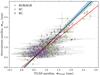Fig. 1

Comparison between asteroseismic and TGAS parallaxes. The markers indicate the evolutionary state of the star, including the red giant branch (RGB or AGB), the red clump (RC), and the secondary clump (SC). The red line shows the 1:1 relation. The black line shows the linear relation obtained from an orthogonal distance regression (ODR), which includes uncertainties on both parallax estimates. The best-fitting relation is ϖ_seis = (1.21 ± 0.07) × ϖ_TGAS−(0.12 ± 0.08). The shaded blue region shows the 1-σ confidence interval around the best-fitting relation.

Open with DEXTER

2. The asteroseismic constraints

Asteroseismology provides two key sets of constraints that may be used as independent ways of inferring distances:

Radii of red giant stars can be estimated from the averageasteroseismic parameters that characterize their acousticoscillation spectra: the so-called average large frequencyseparation, and the frequency corresponding to the maximumobserved oscillation power. Red giants, which show thesesolar-like oscillations, may therefore be used as accurate distanceindicators, just as in the case of eclipsing binaries; the distance toeach red giant may be estimated from the absolute luminosity,which is obtained from the asteroseismically determined radius(for example from asteroseismic scaling relations) andT_eff (e.g., Miglio et al. 2013).
Thanks to the frequencies of dipolar gravito-acoustic modes we can discern pristine RC stars among the zoo of red-giant stars (Bedding et al. 2011). We note that these inferences are independent of the constraints used to determine radii (and hence distances). Once RC stars are identified, their distances may be determined given their intrinsic luminosity.

RC stars in the solar neighborhood are expected to have similar intrinsic K_s-band luminosities (to within ~ 0.2 mag). Therefore, we anticipate a RC-coherent, extended feature in a diagram showing distance and apparent luminosity. This feature would show the expected distance dependence subject to some scatter or offset from the effects of reddening (photometric-band-dependent), stellar multiplicity, and the intrinsic scatter of RC luminosities.

We adopt a set of asteroseismic distances calculated using a model-independent method, that is, using the asteroseismic scaling relations (e.g., Miglio et al. 2013); they are tabulated as the “distances from direct method” in the online data provided by R14. This method assumes no knowledge of the evolutionary state of the star and being model-independent does not force the estimated luminosities to some assumed RC value. This ensures that we have an independent estimate of luminosity for each star to use as a test of the assumption that the RC has a low scatter in luminosity.

We selected our RC sample using an asteroseismic classification (Elsworth et al. 2016) that exploits the diagnostic properties of dipole modes of mixed character, allowing one to discriminate between hydrogen-shell and helium core-burning red giant stars (Bedding et al. 2011). This classification has been shown to be robust in the identification of RC stars and is capable of separating out secondary clump stars and, with the addition of temperature from Pinsonneault et al. (2014), the horizontal branch stars.

3. Results

Figure 2 shows the results of using a sample of RC stars as tests of the asteroseismic and astrometric distance scales. We calculate the theoretical dependence of the apparent K_s-band magnitudes of the RC stars on distance (and hence parallax, i.e., ϖ = 1000 /d, with d in parsecs – in Fig. 2 the dashed red line) using: 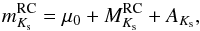(1)where are apparent K_s magnitudes obtained from the Two Micron All Sky Survey (2MASS; Cutri et al. 2003; Skrutskie et al. 2006); μ₀ = 5log ₁₀(d)−5 is the distance modulus; A_{K_s} is the interstellar extinction in the K_s band, determined from E(B−V) reddening values from the 3D dust map by Green et al. (2015; derived from stars in the Pan-STARRS 1 survey) at the asteroseismic distance of a given star and we adopted an extinction-to-reddening ratio of R_{K_s} = 0.355 ± 0.1 (Fitzpatrick 1999). The maximum value of A_{K_s} from the Green et al. (2015) map of our RC sample is 0.08, with a mean of A_{K_s} ≈ 0.02. is the absolute K_s band magnitude for the RC population (see Girardi 2016, and references therein); we adopted a median of the literature values presented in Girardi (2016), that is, , where the uncertainty includes the RMS scatter between the different values. For the six RC stars added from the M67 cluster, we de-reddened the K_s magnitudes using E(B−V) = 0.041 ± 0.004 (Taylor 2007), and for the asteroseismic distance, we adopted the value given by Stello et al. (2016) of d = 816 ± 11 pc.

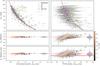Fig. 2

Top: relation between asteroseismic (left) or TGAS (right) parallaxes and de-reddened 2MASS K_s magnitudes (m_{K_s}) for our sample. The markers indicate the evolutionary state of the star, including the red giant branch (RGB or AGB), the red clump (RC), and the secondary clump (SC). We note that the uncertainties on m_{K_s} are typically smaller than the marker size. The dashed red line in both panels shows the theoretical relation used for the residuals in the bottom panels. The relation is given by Eq. (1) using the median theoretical value of from the literature (see Girardi 2016, and references therein); the gray regions around the relations indicate the span of the literature values. The filled red markers denote the six asteroseismic RC stars in the M67 cluster (Stello et al. 2016) for which TGAS parallaxes were available. The middle panel shows fractional differences between the observed and predicted m_{K_s} magnitudes from Eq. (1) at the asteroseismic (left) and TGAS (right) parallaxes of the RC stars. The bottom panel shows residuals between observed and predicted parallaxes from Eq. (1) at the asteroseismic (left) and TGAS (right) parallaxes of the RC stars. The red dash-dot lines and shaded confidence regions follow the predicted offset of −0.39 ± 0.08 mas of the TGAS parallaxes by Stassun & Torres (2016), adopting the ecliptic latitude β = 55° ± 5 of the Kepler field-of-view. The inserts in the middle and bottom panels are violin plots of the distributions of the fractional differences and residuals, with the horizontal black lines giving the median values; the colors indicate the m_{K_s} magnitudes.

Open with DEXTER

In the left-hand panels of Fig. 2, the agreement of the asteroseismic parallax scale with the expected relation demonstrates that a sample of RC stars together with m_{K_s} can be used to test the distance scale. There is, in contrast, a clear systematic error in the TGAS parallaxes versus distance, even given the large scatter.

For the M67 RC stars, we see noticeable differences in parallaxes when compared with the expected values. We note that while it is possible to suggest a correction to the TGAS parallaxes (see Sect. 4), it is difficult to see how a correction based solely on parallax or some measure of color could solve the problem presented by the M67 RC stars.

To check for the effects of extinction, binarity, and RC population heterogeneity on the results, we have generated a synthetic population with the properties expected of the Kepler field (see Miglio et al. 2014). Figure 3 plots K_s-band apparent magnitudes as a function of parallax for a TRILEGAL simulated population (Girardi et al. 2005) of single RC stars. The expected dependence is clear, as is the intrinsic spread in the RC K_s luminosity (see Eq. (1)). The extinction in the K_s band, A_{K_s}, was determined from the A_V values in TRILEGAL and R_{K_s} = 0.355 ± 0.1 (as per the real data) and R_V = 3.1 ± 0.1 (Cardelli et al. 1989).

As expected, for the small values of extinction expected here, band extinction has little effect on the inferred asteroseismic distances (when using the K_s). We investigated the impact of a poorly estimated extinction by changing the true extinction by a factor of two. The results of this test show that even with this large systematic error in extinction, the impact on the estimated distances is of the order of only a few percent.

We have also used the synthetic population to estimate the impact of unresolved binaries on the apparent K_s-band magnitudes. We find that only for a few systems (<1%), with luminosity ratios close to unity, does the change in apparent magnitude significantly impact the asteroseismic distance estimate. It is worth noting that later releases of Gaia parallaxes are expected to achieve sufficiently high precision that the tests here could be used to identify unresolved binaries and constrain interstellar reddening.

	Fig. 3 As for Fig. 2 but with a simulated RC population.
Open with DEXTER

4. Suggested correction

Using the sample of RC stars, we propose a correction to the TGAS parallaxes. We find that the median offset between the TGAS parallaxes and the values predicted from Eq. (1) is very close to −0.1 mas (in the sense that TGAS overestimates the distance), which is less than either the −0.39 mas correction for the Kepler field ecliptic latitude or the bulk offset of −0.25 mas given by Stassun & Torres (2016). However, we see the bias decrease at smaller parallaxes, and at parallaxes larger than ~ 1.6 mas, our correction is comparable to that of Stassun & Torres (2016).

Figure 4 shows the correction we propose that should be added to the TGAS parallaxes in the Kepler field as a function of the theorectical RC parallax, that is, the parallax that would be returned by an accurate estimate of the distance, ϖ_dist: 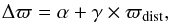(2)with parameters α = −0.15 ± 0.06, γ = 0.29 ± 0.06, and a parameter correlation of r_α,γ ≈ −0.95. Uncertainties were estimated from the ODR. The correction may, in practice, be applied in an iterative manner. One begins by adopting ϖ_TGAS = ϖ_dist to compute a correction Δϖ using Eq. (1), and hence a corrected parallax. This corrected parallax is then used as an input to Eq. (1) to compute a new correction, and an iterated corrected parallax. The process is repeated until good convergence is found (typically this requires only one or two iterations).

This correction is calibrated with Kepler data and hence is strictly applicable to stars in the Kepler field. If, as suggested by Stassun & Torres (2016), any correction of TGAS parallaxes should be a function of ecliptic latitude, then the correction could be extended to all stars at similar latitudes. Care should be taken if this correction is to be applied at different latitudes.

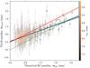Fig. 4

Parallaxes predicted from Eq. (1) at the m_{K_s} magnitudes of the RC stars and those of TGAS. The full red line shows the 1:1 relation. The black lines give the linear fit between the parallaxes with the associated 1-σ uncertainty given by the blue shaded regions. The green dashed line shows the predicted off-set of −0.39 mas from Stassun & Torres (2016), adopting an ecliptic latitude of β = 55° of the Kepler field-of-view. The marker colors indicate the m_{K_s} magnitudes of the stars. The correction of Eq. (2) is given by the difference between the 1:1 relation and the linear fit.

Open with DEXTER

5. Conclusions

In this letter, we have used red clump (RC) stars as distance estimators to test the systematic error in the Gaia DR1 TGAS sample. We have reproduced the results of De Ridder et al. (2016) showing there is a disagreement between the TGAS distances and asteroseismic distances. By testing both results against the RC distance scale we have demonstrated that the asteroseismic distances are in better agreement with the RC than the TGAS distances. The TGAS sample showed a median offset of approximately −0.1 mas (in the sense that TGAS overestimates the distance). We have also considered six RC stars with asteroseismic detections in the open cluster M67 but find discrepancies in the TGAS parallaxes that would be challenging to explain in terms of a color or spatially motivated systemic error.

We have proposed a correction to the TGAS parallaxes as a function of distance (as described by parallax). This correction is applicable to the Kepler field-of-view at distances > 500 pc, but could be used at similar ecliptic latitudes (β = 55° ± 5) following the findings of Stassun & Torres (2016). Care should be exercised when applying this correction to other latitudes should the TGAS bias be position dependent. The correction we find converges to the Stassun & Torres (2016) correction at parallaxes larger that ~ 1.6 mas, but is noticeably smaller at greater distances.

Our results then bridge the gap between both the previous works that favor a correction but are sensitive to nearby stars (Stassun & Torres 2016; Jao et al. 2016) and works that favor no correction but are sensitive to more distant stars (Lindegren et al. 2016; Sesar et al. 2016). We conclude that a correction to the TGAS sample is required but that this correction becomes negligible at distances greater than ~ 1.2 kpc.

Acknowledgments

We thank J. de Ridder, D. Huber, J. Heifetz and the anonymous referee for their help and useful comments. This publication is a direct result of a hack session organised in the Solar and Stellar Physics group at the University of Birmingham. This work has made use of data from the European Space Agency (ESA) mission Gaia (http://www.cosmos.esa.int/gaia), processed by the Gaia Data Processing and Analysis Consortium (DPAC, http://www.cosmos.esa.int/web/gaia/dpac/consortium). Funding for the DPAC has been provided by national institutions, in particular the institutions participating in the Gaia Multilateral Agreement. The authors acknowledge the support of the UK Science and Technology Facilities Council (STFC). M.N.L. acknowledges the support of The Danish Council for Independent Research | Natural Science (Grant DFF-4181-00415). Funding for the Stellar Astrophysics Centre (SAC) is provided by The Danish National Research Foundation (Grant DNRF106). L.G. and T.S.R. acknowledge support from PRIN INAF 2014 (CRA 1.05.01.94.05)

References

Bedding, T. R., Mosser, B., Huber, D., et al. 2011, Nature, 471, 608 [NASA ADS] [CrossRef] [PubMed] [Google Scholar]
Boggs, P. T., & Rogers, J. E. 1990, Contemporary Mathematics, 112, 183 [CrossRef] [Google Scholar]
Cannon, R. D. 1970, MNRAS, 150, 111 [NASA ADS] [CrossRef] [Google Scholar]
Cardelli, J. A., Clayton, G. C., & Mathis, J. S. 1989, ApJ, 345, 245 [NASA ADS] [CrossRef] [Google Scholar]
Cutri, R. M., Skrutskie, M. F., van Dyk, S., et al. 2003, VizieR Online Data Catalog: II/246 [Google Scholar]
De Ridder, J., Molenberghs, G., Eyer, L., & Aerts, C. 2016, A&A, 595, L3 [NASA ADS] [CrossRef] [EDP Sciences] [Google Scholar]
Elsworth, Y., Hekker, S., Basu, S., & Davies, G.-R. 2016, MNRAS, submitted [Google Scholar]
Fitzpatrick, E. L. 1999, PASP, 111, 63 [NASA ADS] [CrossRef] [Google Scholar]
Gaia Collaboration (Brown, A. G. A., et al.) 2016, A&A, 595, A2 [NASA ADS] [CrossRef] [EDP Sciences] [Google Scholar]
Girardi, L. 2016, ARA&A, 54, 95 [NASA ADS] [CrossRef] [Google Scholar]
Girardi, L., Groenewegen, M. A. T., Hatziminaoglou, E., & da Costa, L. 2005, A&A, 436, 895 [NASA ADS] [CrossRef] [EDP Sciences] [Google Scholar]
Green, G. M., Schlafly, E. F., Finkbeiner, D. P., et al. 2015, ApJ, 810, 25 [NASA ADS] [CrossRef] [Google Scholar]
Jao, W.-C., Henry, T. J., Riedel, A. R., et al. 2016, ApJ, 832, L18 [NASA ADS] [CrossRef] [Google Scholar]
Lindegren, L., Lammers, U., Bastian, U., et al. 2016, A&A, 595, A4 [NASA ADS] [CrossRef] [EDP Sciences] [Google Scholar]
Michalik, D., Lindegren, L., & Hobbs, D. 2015, A&A, 574, A115 [NASA ADS] [CrossRef] [EDP Sciences] [Google Scholar]
Miglio, A., Chiappini, C., Morel, T., et al. 2013, MNRAS, 429, 423 [NASA ADS] [CrossRef] [Google Scholar]
Miglio, A., Chaplin, W. J., Farmer, R., et al. 2014, ApJ, 784, L3 [NASA ADS] [CrossRef] [Google Scholar]
Paczyński, B., & Stanek, K. Z. 1998, ApJ, 494, L219 [NASA ADS] [CrossRef] [Google Scholar]
Pinsonneault, M. H., Elsworth, Y., Epstein, C., et al. 2014, ApJS, 215, 19 [NASA ADS] [CrossRef] [Google Scholar]
Rodrigues, T. S., Girardi, L., Miglio, A., et al. 2014, MNRAS, 445, 2758 [NASA ADS] [CrossRef] [Google Scholar]
Salaris, M., & Girardi, L. 2002, MNRAS, 337, 332 [NASA ADS] [CrossRef] [Google Scholar]
Sesar, B., Fouesneau, M., Price-Whelan, A. M., et al. 2016, ApJ, submitted [arXiv:1611.07035] [Google Scholar]
Skrutskie, M. F., Cutri, R. M., Stiening, R., et al. 2006, AJ, 131, 1163 [NASA ADS] [CrossRef] [Google Scholar]
Stassun, K. G., & Torres, G. 2016, ApJ, submitted [arXiv:1609.05390] [Google Scholar]
Stello, D., Vanderburg, A., Casagrande, L., et al. 2016, ApJ, 832, 133 [NASA ADS] [CrossRef] [Google Scholar]
Taylor, B. J. 2007, AJ, 133, 370 [NASA ADS] [CrossRef] [Google Scholar]

All Figures

	Fig. 1 Comparison between asteroseismic and TGAS parallaxes. The markers indicate the evolutionary state of the star, including the red giant branch (RGB or AGB), the red clump (RC), and the secondary clump (SC). The red line shows the 1:1 relation. The black line shows the linear relation obtained from an orthogonal distance regression (ODR), which includes uncertainties on both parallax estimates. The best-fitting relation is ϖ_seis = (1.21 ± 0.07) × ϖ_TGAS−(0.12 ± 0.08). The shaded blue region shows the 1-σ confidence interval around the best-fitting relation.
Open with DEXTER
In the text

	Fig. 2 Top: relation between asteroseismic (left) or TGAS (right) parallaxes and de-reddened 2MASS K_s magnitudes (m_{K_s}) for our sample. The markers indicate the evolutionary state of the star, including the red giant branch (RGB or AGB), the red clump (RC), and the secondary clump (SC). We note that the uncertainties on m_{K_s} are typically smaller than the marker size. The dashed red line in both panels shows the theoretical relation used for the residuals in the bottom panels. The relation is given by Eq. (1) using the median theoretical value of from the literature (see Girardi 2016, and references therein); the gray regions around the relations indicate the span of the literature values. The filled red markers denote the six asteroseismic RC stars in the M67 cluster (Stello et al. 2016) for which TGAS parallaxes were available. The middle panel shows fractional differences between the observed and predicted m_{K_s} magnitudes from Eq. (1) at the asteroseismic (left) and TGAS (right) parallaxes of the RC stars. The bottom panel shows residuals between observed and predicted parallaxes from Eq. (1) at the asteroseismic (left) and TGAS (right) parallaxes of the RC stars. The red dash-dot lines and shaded confidence regions follow the predicted offset of −0.39 ± 0.08 mas of the TGAS parallaxes by Stassun & Torres (2016), adopting the ecliptic latitude β = 55° ± 5 of the Kepler field-of-view. The inserts in the middle and bottom panels are violin plots of the distributions of the fractional differences and residuals, with the horizontal black lines giving the median values; the colors indicate the m_{K_s} magnitudes.
Open with DEXTER
In the text

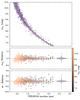	Fig. 3 As for Fig. 2 but with a simulated RC population.
Open with DEXTER
In the text

	Fig. 4 Parallaxes predicted from Eq. (1) at the m_{K_s} magnitudes of the RC stars and those of TGAS. The full red line shows the 1:1 relation. The black lines give the linear fit between the parallaxes with the associated 1-σ uncertainty given by the blue shaded regions. The green dashed line shows the predicted off-set of −0.39 mas from Stassun & Torres (2016), adopting an ecliptic latitude of β = 55° of the Kepler field-of-view. The marker colors indicate the m_{K_s} magnitudes of the stars. The correction of Eq. (2) is given by the difference between the 1:1 relation and the linear fit.
Open with DEXTER
In the text

Current usage metrics show cumulative count of Article Views (full-text article views including HTML views, PDF and ePub downloads, according to the available data) and Abstracts Views on Vision4Press platform.

Data correspond to usage on the plateform after 2015. The current usage metrics is available 48-96 hours after online publication and is updated daily on week days.

Initial download of the metrics may take a while.