| Issue |
A&A
Volume 598, February 2017
|
|
|---|---|---|
| Article Number | A102 | |
| Number of page(s) | 12 | |
| Section | Atomic, molecular, and nuclear data | |
| DOI | https://doi.org/10.1051/0004-6361/201629849 | |
| Published online | 08 February 2017 | |
Experimental and theoretical oscillator strengths of Mg i for accurate abundance analysis
1 Materials Science and Applied Mathematics, Malmö University, 205 06 Malmö, Sweden
e-mail: asli.pehlivan@mah.se; asli@astro.lu.se
2 Lund Observatory, PO Box 43, 221 00 Lund, Sweden
Received: 5 October 2016
Accepted: 18 November 2016
Context. With the aid of stellar abundance analysis, it is possible to study the galactic formation and evolution. Magnesium is an important element to trace the α-element evolution in our Galaxy. For chemical abundance analysis, such as magnesium abundance, accurate and complete atomic data are essential. Inaccurate atomic data lead to uncertain abundances and prevent discrimination between different evolution models.
Aims. We study the spectrum of neutral magnesium from laboratory measurements and theoretical calculations. Our aim is to improve the oscillator strengths (f-values) of Mg i lines and to create a complete set of accurate atomic data, particularly for the near-IR region.
Methods. We derived oscillator strengths by combining the experimental branching fractions with radiative lifetimes reported in the literature and computed in this work. A hollow cathode discharge lamp was used to produce free atoms in the plasma and a Fourier transform spectrometer recorded the intensity-calibrated high-resolution spectra. In addition, we performed theoretical calculations using the multiconfiguration Hartree-Fock program ATSP2K.
Results. This project provides a set of experimental and theoretical oscillator strengths. We derived 34 experimental oscillator strengths. Except from the Mg i optical triplet lines (3p 3P°0,1,2–4s 3S1), these oscillator strengths are measured for the first time. The theoretical oscillator strengths are in very good agreement with the experimental data and complement the missing transitions of the experimental data up to n = 7 from even and odd parity terms. We present an evaluated set of oscillator strengths, gf, with uncertainties as small as 5%. The new values of the Mg i optical triplet line (3p 3P°0,1,2–4s 3S1) oscillator strength values are ~0.08 dex larger than the previous measurements.
Key words: atomic data / methods: laboratory: atomic / techniques: spectroscopic
© ESO, 2017
1. Introduction
Magnesium is an important element for chemical evolution studies. It is an α-element, which is formed and released during supernova type II explosions of massive stars. Magnesium lines are strong in the spectra of late-type stars and even in metal-poor stars. Therefore, it is an ideal element to trace the α-element abundances.
The dominant electron source in the stellar atmospheres of metal-poor stars is magnesium. As a result, its abundance affects the model atmospheres (Prochaska et al. 2000). The higher the magnesium abundance, the higher the electron density becomes in the stellar atmosphere. Neglecting this fact may lead to incorrect stellar gravity determination. Prochaska et al. (2000) used an α-enhanced model atmosphere to derive abundances. For magnesium abundance analysis, they only found very few magnesium lines with reported log (gf) values. Because of the missing data, they included additional lines with astrophysical log (gf) values.
Several studies (Shigeyama & Tsujimoto 1998; Bensby et al. 2003; Cayrel et al. 2004; Andrievsky et al. 2010) have used magnesium as an alternative to iron for tracing the chemical evolution of the Milky Way. Magnesium is only formed in supernova type II explosions of massive stars (Woosley & Weave 1995), whereas iron has several formation channels (Thielemann et al. 2002). A complete set of magnesium atomic data results in more accurate abundances and, correspondingly, makes magnesium an even better choice as a tracer of galactic evolution.
At temperatures T ≥ 5000 K, magnesium is primarily singly ionised. However there are a large number of Mg i lines existing in the solar spectrum (Scott et al. 2015). As a result of Mg+ being the dominant species, Mg i is sensitive to the deviations from local thermodynamic equilibrium (LTE). In particular, for the metal-poor stars these non-LTE (NLTE) effects are predicted to be significant (Zhao et al. 1998; Zhao & Gehren 2000). To study the deviations from LTE, It is crucial to have accurate atomic data of both Mg i and Mg ii. This makes it possible to map the limits of LTE approximations as a function of stellar metallicity, gravity, and temperature, similar to Fe i in Lind et al. (2012). There are several studies on NLTE analysis of neutral magnesium including the recent studies of Bergemann et al. (2015), Osorio & Barklem (2016). The former studied NLTE effects in the J-band Mg i lines and, due to a lack of experimental log (gf) values, calculated log (gf) values were used. However, using the average of the many calculated log (gf) values overestimated the line depths, Bergemann et al. (2015) concluded that the values were wrong and derived their astrophysical log (gf) values.
Scott et al. (2015) determined the magnesium abundance of the Sun to be log ϵMg = 7.59 ± 0.04 from a 3D hydrodynamic model of the solar photosphere. However, due to the lack of laboratory measurements of log (gf) values, they used theoretical log (gf) values of Butler et al. (1993) and Chang & Tang (1990). The current study provides experimental log (gf) values for two of the lines and improved theoretical log (gf) values for all the lines used by Scott et al. (2015).
In addition, some planetary atmosphere studies show the presence of magnesium in the atmospheres of planets (Fossati et al. 2010; Vidal-Madjar et al. 2013; Bourrier et al. 2014, 2015). By analysing the resonance line of an abundant element, such as magnesium, during a planet transit, the atmospheric escape mechanism can be understood. These studies are usually done by analysing absorption depths of the line of interest, which requires accurate atomic data.
To our knowledge there are no experimental oscillator strengths of Mg i lines, except from the 3s2
 intercombination transition at 4571 Å (Kwong et al. 1982) and the Mg i triplets lines (3p 3P
 –4s 3S1); 5167, 5172, and 5183 Å (Aldenius et al. 2007). Although Ueda et al. (1982) provided oscillator strengths for the transitions from 3p 3P level, they were not completely experimental values. Theoretical calculations in Wiese et al. (1969) compilation were used for the absolute scale of the oscillator strengths.
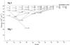 |
Fig. 1 Partial energy level diagram of Mg i with dashed lines showing the observed transitions. The energy level values are from Martin & Zalubas (1980). |
There are several theoretical values, which are generally used for abundance analysis. Chang & Tang (1990) calculated oscillator strengths of Mg i lines between selected 1,3S–1,3F states using the configuration interaction (CI) procedure with a finite basis set constructed from B splines. In addition, theoretical values of Butler et al. (1993) are commonly used for abundance analyses. They used the close-coupling approximation with the R-matrix technique. Moreover, Civiš et al. (2013) performed oscillator strength calculations using the quantum defect theory (QDT) in the region of 800–9000 cm-1. Froese Fischer et al. (2006) performed calculations using the multi configuration Hartree-Fock method. Their calculations included the terms up to n = 4 and all three types of correlations: valence, core-valence, and core-core correlation.
This paper presents experimental log (gf) values of Mg i lines from high-resolution laboratory measurements in the infrared and optical region from the upper even parity 4s 1,3S, 5s 1S, 3d 1D, and 4d 1D terms and the odd parity 4p 3P°, 5p 3P°, 4f 1,3F°, and 5f 1,3F° terms. In addition, we performed multiconfiguration Hartree-Fock calculations using the ASTP2K package (Froese Fischer et al. 2007) and obtained log (gf) values of Mg i lines up to n = 7 from even parity 1,3S, 1,3D, and 1,3G terms and odd parity 1,3P°, and 1,3F° terms. The transitions between the higher terms fall in the IR spectral region and the calculated log (gf) values are important for interpreting observations using the new generation of telescopes designed for this region. Following the introduction, Sect. 2 describes the experimental method we used for deriving log (gf) values. In addition, this section explains the measurements of branching fractions (BF) and the uncertainty estimations. The theoretical calculations that we performed are explained in Sect. 3. In Sect. 4, we present our results, the comparisons of our results with previous studies, and the conclusions.
2. Experimental method
We used a water-cooled hollow cathode discharge lamp (HCL) with a magnesium cathode as a light source to produce the magnesium plasma. The experimental set-up was similar to the one described by Pehlivan et al. (2015). The strongest lines for the measurements were obtained using neon as carrier gas and with an applied current of 0.60 A.
We recorded the Mg i spectra with the high-resolution Fourier transform spectrometer (FTS), Bruker IFS 125 HR, at the Lund Observatory (Edlén Laboratory). The maximum resolving power of the instrument is 106 at 2000 cm-1 and the covered wavenumber region is 50 000–2000 cm-1 (200–5000 nm). We set the resolution to 0.01 cm-1 during the measurements and recorded the spectra with indium antimonide (InSb), silicon (Si), and photomultiplier tube (PMT) detectors. These detectors are sensitive to different spectral regions, but they overlap each other in a small wavelength region.
The optical element contributions to the FTS response function were compensated for by obtaining an intensity calibration. Because of the wavelength-dependent transmission of the optical elements and the spectrometer, the measured intensities of the lines differ from their intrinsic intensities. Therefore, we acquired the response function of the instrument for three different detectors that we used during different measurements. The response function is usually determined by measuring the spectrum of an intensity calibrated reference lamp. We used a tungsten filament lamp for the intensity calibration of Mg i lines. The lamp was calibrated by the Swedish National Laboratory (SP) for spectral radiance in the region between 40 000−4000 cm-1 (250−2500 nm). With the calibrated radiance of the lamp, the response function of the instrument can be determined for different detectors. We used the overlapping region Mg i lines, which were recorded with different detectors, to connect the relative intensities on the same scale. This was done by using a normalisation factor nf, which in turn contributed an additional uncertainty to the BFs.
In addition, we recorded the spectra with different currents to compensate for self-absorption effects. The self-absorption affects the intensity of the line and this, in turn, influences the BF measurements which are used to determine the oscillator strengths. More details can be found in our previous paper (Pehlivan et al. 2015).
2.1. Branching fraction measurements
The oscillator strength of a spectral line is proportional to the transition probability. For electric dipole transition, it is given as  (1)where gu is the statistical weight of the upper level, gl the statistical weight of the lower level, λ the wavelength of the transition in Å, and Aul the transition probability between the upper level u and the lower level l in s-1.
The radiative lifetime of an upper level, τu is the inverse of the sum of all transition probabilities from the same upper level, τu = 1/ ∑ iAui. The branching fraction (BF) of a line is defined as the transition probability of the line Aul divided by the total transition probability of the lines from the same upper level;  (2)As the transition probability is proportional to the line intensity Iul, BF can be defined as the ratio of the line intensities.
Knowing the radiative lifetime and combining this with the measured BFs, one can derive the transition probability, Aul, of a spectral line;  (3)Transitions from the same upper level can have wavelengths belonging to different regions of the electromagnetic spectrum. However, to accurately measure BFs, all transitions from the same upper level should be accounted for. For this reason, we recorded Mg i spectra using different detectors. These different spectra were put on the same relative intensity scale by using a normalisation factor.
A partial energy level diagram of Mg i levels is shown in Fig. 1. The transitions, which we observed and used to derive log (gf) values, are marked in this figure. Using the Kurucz (2009) database and references in Kaufman & Martin (1991), we predicted the Mg i lines from the same upper level. We identified these lines and analysed our recorded spectra with the FTS analysis software GFit (Engström 1998, 2014).
Mg i has three dominant isotopes: 24Mg with 78.99% abundance, 25Mg with 10% abundance, and 26Mg with 11% abundance (IUPAC 1991). Although there are three isotopes of Mg i, in our measurements we did not see any isotope shift. The nuclear spins of these isotopes are 0, 5/2, and 0, respectively. This proves that the most dominant isotope 24Mg has no hyperfine splitting (hfs) in the line profiles. Even though 25Mg has a nuclear spin of 5/2, we did not see any hfs as the abundance of this isotope is very low compared to 24Mg.
2.2. Uncertainties
The uncertainty of the BF contains several components. Together with the uncertainty of the intensities, the uncertainty of the self-absorption correction, the uncertainty of the intensity calibration lamp, and the uncertainty of the normalisation factor, which is used to put the intensities on the same scale, should be considered. Including all of these uncertainty components, Sikström et al. (2002) defined the total uncertainty of the BF as, 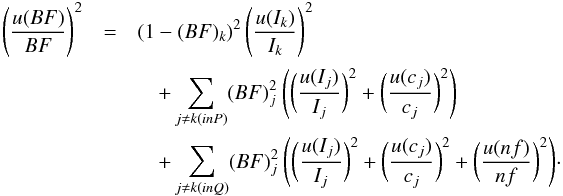 (4)The first term of the equation includes the branching fraction (BF)k of the line of interest in the spectral region of the detector P and the uncertainty in the measured intensity of the same line, u(Ik). In the sum that follows u(cj) and u(Ij) are the uncertainties of the calibration lamp and the uncertainties of the measured intensities, respectively, for other lines from the same upper level recorded with the detector P. (BF)j are the branching fractions. The last sum, that describes uncertainties from lines recorded with detector Q, also includes the uncertainty u(nf) in the normalisation factor nf connecting different spectral regions. The intensity uncertainties from the statistical noise were determined using GFit. They varied between 0.001% for the strong lines and ~ 20% for the weak lines or self-absorbed lines. Most of the lines have uncertainties below 1%. When there was self-absorption, we corrected these lines and added the uncertainty from self-absorption to the intensity uncertainty. The calibration lamp uncertainty is 7% and the uncertainty of the normalisation factor is 5%. From propagation of errors and using Eq. (3), the uncertainty of the transition probability or f-value is defined as,
 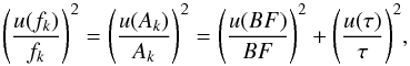 (5)where u(τ) is the uncertainty of the radiative lifetime of the upper level. In the cases where we used experimental lifetimes of Jönsson et al. (1984), the uncertainties vary between 5% and 7%. For the theoretical lifetime uncertainties, we compared our theoretical values (to be described in the following section) with the experimental lifetimes available in the literature (Kwiatkowski et al. 1980; Jönsson et al. 1984; Larsson & Svanberg 1993; Larsson et al. 1993; Aldenius et al. 2007). Figure 2 shows the comparison of the experimental lifetime values with the theoretical lifetime values that we calculated. The blue dashed line marks the 15% and the black dashed line marks the 10% difference. As the difference is small, we adopted 10% relative uncertainty for the theoretical lifetimes.
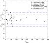 |
Fig. 2 Comparison of the theoretical lifetimes of this study with the previously measured experimental lifetimes. As seen in the figure, there is a large difference of almost 20% for one of the values measured by Aldenius et al. (2007). However, a re-measurement of the lifetime brings it in a very good agreement with the calculated value (see text for more details). |
3. Theoretical method
We performed our calculations using the multiconfiguration Hartree-Fock method (MCHF; Froese Fischer et al. 1997, 2016). In this method , atomic state functions (ASF) Ψ(γLS) for the LS terms are represented by linear combinations of configuration state functions (CSF); 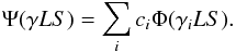 (6)In the equation, γ represents the electronic configurations and the quantum numbers other than L and S. The configuration state functions Φ(γiLS) are built from one-electron orbitals and ci are the mixing coefficients. The mixing coefficients and the radial parts of the one-electron orbitals are determined by solving a set of equations that results from applying the variational principle to the energy expression associated with the ASFs.
We started with a calculation of the ASFs describing terms of the configurations with n up to nine and l up to g such as 3s2, 3s3p, 3s3d, ..., 3s9g. The calculation was done in the simplest approximation, where each ASF consists of only one CSF. All the ASFs were determined together in the same run and the calculation yielded a number of orbitals that were kept fixed in the proceeding calculations.
Terms involving configurations with n = 8,9 were not our prime target. However, we included these terms in the initial calculation to obtain orbitals that are spatially localised far away from the nucleus. This leads to a more complete and balanced orbital set. To improve the ASFs describing terms of the configurations with n up to seven and l up to g, such as 3s2, 3s3p, 3s3d, ..., 3s7g, we performed calculations with systematically enlarged CSF expansions. These expansions were formed from single and double replacements of orbitals in the reference configurations with orbitals in an active orbital set. We applied restrictions that there should be at most one replacement from 2s22p6 and 1s2 should be a closed shell. The orbitals in the active set were extended to include orbitals with n = 13 and l = h. In these calculations, we determined ASFs with the same LS symmetry together.
Once the ASFs were determined, the oscillator strengths were calculated as expectation values of the transition operator. We performed the calculations both in the length and in the velocity gauge; see Froese Fischer et al. (1997) for more details. For accurate calculations, the oscillator strengths in the two gauges should give the same value. In our calculations, the oscillator strengths in the two gauges typically agree to within 5% for transitions between low-lying terms. The agreement is slightly worse for transitions involving the highest terms. Nevertheless, the velocity gauge, which weights more to the inner part of the wave function, shows good convergence properties and is believed to be the more accurate one for transitions involving the more excited states.
All calculations were non-relativistic and the obtained gf values represent term averages. To obtain the gf values for the fine-structure transitions rather than for transitions between terms, we multiplied the gf values for the term averages with the square of the line factor, see Cowan (1981, Eq. (14.50)).
Moreover, we investigated the influence of relativistic effects by comparing our results with results from calculations where relativistic effects were accounted for in the Breit-Pauli approximation. As expected, the relativistic effects were insignificant with negligible term mixing. Exceptions are the J = 3 states of the 1,3F terms in which the energy separations are so small that even weak relativistic effects give considerable term mixing. For the states of 4f 1,3F terms, we performed full calculations with relativistic effects in the Breit-Pauli method and applied the method of fine tuning (Brage & Hibbert 1989) to match with the experimental data of Martin & Zalubas (1980). Due to the very small energy separations, it was not possible to perform these calculations for the higher n and thus no theoretical oscillator strength values are given for states of the 5f, 6f, 7f 1,3F terms.
4. Results and conclusions
In this study, experimental and theoretical oscillator strengths of Mg i are provided. BFs were obtained using Eq. (2) from the observed line intensities. We recorded the spectra using different currents and detectors. Applying different currents helped to rule out any self-absorption effects. The spectra, which are recorded with different detectors, are put on the same intensity scale by using a normalisation factor. In this way, we had all the lines from the same upper level on the same intensity scale. In the cases where we had unobservable weak lines, we used the theoretical transition probabilities to estimate the residual values.
From the measured BFs and radiative lifetimes, the transition probabilities Aul are derived using Eq. (3) and log (gf) values are derived from Eq. (1). For the experimental lifetimes, we used the values of Jönsson et al. (1984), and for others we used our theoretical radiative lifetimes. Table 1 shows the theoretical lifetime values we computed together with the previous experimental and theoretical lifetime values. One notes that sometimes there are very large differences between values by Kurucz (2009) and the experimental values.
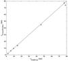 |
Fig. 3 Comparison between lifetime values of Froese Fischer et al. (2006) and this work. |
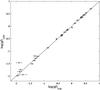 |
Fig. 4 Comparison between experimental and theoretical log(gf) values of this work. The theoretical and experimental log (gf) values differ markedly for two transitions. These two transitions are affected by a blend and thus the derived experimental values are very uncertain (see text for more details). |
Theoretical radiative lifetimes of this work together with previous theoretical and experimental lifetimes.
Figure 2 shows a comparison of our theoretical lifetime values with experimental work of Kwiatkowski et al. (1980), Jönsson et al. (1984), Larsson & Svanberg (1993), Larsson et al. (1993), Aldenius et al. (2007). Overall, our calculations agree with the previously published experimental values within the 10% uncertainty. Furthermore, we compared our lifetime values with the theoretical values from Froese Fischer et al. (2006) in Fig. 3 and the agreement is very good. Even the largest deviations are less than 6%.
From experimental BFs, we derived 34 log (gf) values of Mg i lines from the upper even parity 4s 1,3S, 5s 1S, 3d 1D, and 4d 1D, and odd parity 4p 3P°, 5p 3P°, 4f 1,3F°, and 5f 1,3F° with uncertainties in gf as low as 5%. In addition, we calculated theoretical log (gf) values of Mg i lines up to n = 7 from even parity 1,3S, 1,3D, and 1,3G terms, and odd parity 1,3P° and 1,3F° terms using ATSP2K package. Figure 4 shows the comparison between the experimental and the theoretical log (gf) values. The good agreement between our experimental and theoretical log (gf) values makes us confident to recommend our theoretical values for the transitions in Table A.2. Table A.1 shows our experimental log (gf) values together with their uncertainty and corresponding theoretical log (gf) values that we calculated in this study, together with the branching fractions BF, and the transition probabilities Aul. In addition, we compared our theoretical log (gf) values with Froese Fischer et al. (2006) values in Fig. 5. Froese Fischer et al. (2006) performed calculations for only the lowest lying levels up to n = 4 while the current study calculations are additionally for higher levels up to n = 7. The good agreement between our values and the theoretical values of Froese Fischer et al. (2006) is an additional indication of the quality of our values. Covering much more states and transitions, our calculations complement those of Froese Fischer et al. (2006).
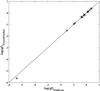 |
Fig. 5 Comparison of log (gf) values of the current study with the values of Froese Fischer et al. (2006). |
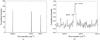 |
Fig. 6 Sample spectrum of two spectral regions of the FTS recordings. a) The Mg i optical triplet lines (3p 3P |

Overall, our theoretical lifetime values are in very good agreement with the experimental lifetime values in the literature. In addition, our theoretical log (gf) values agree with the experimental values of this work. However, our log (gf) values differ from the Aldenius et al. (2007) values for the optical Mg i triplet lines (3p 3P–4s 3S1), although we measured the same BFs. Figure 6 shows these lines in one of our spectra. The difference in log (gf) arises from the radiative lifetime of the upper level. Aldenius et al. (2007) measured the lifetime of 4s3S1 level to 11.5 ± 1.0 ns. Other experimental studies find the lifetime ranging from 5.8 ns to 14.8 ns (Berry et al. 1970; Schaefer 1971; Andersen et al. 1972; Havey et al. 1977; Kwiatkowski et al. 1980). Apparently, there is a large spread in the literature values and a 2 ns difference in lifetime corresponding to a 0.08 dex difference in log(gf) values. The derived log (gf) value is thus sensitive to the choice of lifetime. Using the facility at Lund High Power Laser Centre, we remeasured the lifetime of this level. The atomic structure of Mg i and technical limitations prevented us from deriving a conclusive value. However, the remeasured value leans towards the measurements by Kwiatkowski et al. (1980) and our calculated value. Therefore, we adopted our theoretical lifetime value (9.63 ns) for the 4s3S1 level. Our calculated lifetime value of 9.63 ns is a good choice, because it shows internal consistency between the length and velocity gauges, and in comparisons with other levels. Furthermore, Mashonkina (2013) investigated the atomic data used in stellar magnesium abundance analyses. The paper found that the Aldenius et al. (2007) values overestimate the magnesium abundance by 0.11 dex compared to the other lines. With our experimental values this difference will be reduced.
We recommend our experimental oscillator strengths when available. However, we would like to point out that the uncertainties of the Mg i 15 886.26 Å (6293.03 cm-1) and 15 886.18 Å (6293.06 cm-1) are larger than 20% owing to the weak line intensities and the blending of these two lines with each other. The oscillator strengths of these lines are outliers in Fig. 4. The lines are displayed in Fig. 6. It is seen that they are weak with small separations, making fits to line profiles difficult. For these reasons, we advise the use of theoretical values for these transitions. When the experimental data are not available, we suggest theoretical values to be used.
Acknowledgments
We acknowledge the grant No. 621−2011−4206 from the Swedish Research Council (VR) and Crafoord foundation grant 2015-0947. The infrared FTS at the Edlén laboratory is made available through a grant from the Knut and Alice Wallenberg Foundation. We are grateful to Hans Lundberg for revisiting the laser measurements. A.P.R. acknowledges the travel grant for young researches from the Royal Physiographic Society of Lund. We are grateful for discussions with Paul Barklem, Nils Ryde, and Henrik Jönsson. This project was supported by “The New Milky Way” project from the Knut and Alice Wallenberg foundation.
References
- Aldenius, M., Tanner, J. D., Johansson, S., Lundberg, H., & Ryan, S. G. 2007, A&A, 461, 767 [NASA ADS] [CrossRef] [EDP Sciences] [Google Scholar]
- Andersen, T., Mølhave, L., & Sørensen, G. 1972, ApJ, 178, 577 [NASA ADS] [CrossRef] [Google Scholar]
- Andrievsky, S. M., Spite, M., Korotin, S. A., et al. 2010, A&A, 509, A88 [NASA ADS] [CrossRef] [EDP Sciences] [Google Scholar]
- Bensby, T., Feltzing, S., & Lundström, I. 2003, A&A, 410, 527 [NASA ADS] [CrossRef] [EDP Sciences] [Google Scholar]
- Bergemann, M., Kudritzki, R.-P., Gazak, Z., Davies, B., & Plez, B. 2015, ApJ, 804, 113 [NASA ADS] [CrossRef] [Google Scholar]
- Berry, H. G., Bromander, J., & Buchta, R. 1970, Phys. Scr., 1, 181 [NASA ADS] [CrossRef] [Google Scholar]
- Bourrier, V., Lecavelier des Etangs, A., & Vidal-Madjar, A. 2014, A&A, 565, A105 [NASA ADS] [CrossRef] [EDP Sciences] [Google Scholar]
- Bourrier, V., Lecavelier des Etangs, A., & Vidal-Madjar, A. 2015, A&A, 573, A11 [NASA ADS] [CrossRef] [EDP Sciences] [Google Scholar]
- Brage, T., & Hibbert, A. 1989, J. Phys. B At. Mol. Phys., 22, 713 [Google Scholar]
- Butler, K., Mendoza, C., & Zeippen, C. J. 1993, J. Phys. B At. Mol. Phys., 26, 4409 [NASA ADS] [CrossRef] [Google Scholar]
- Cayrel, R., Depagne, E., Spite, M., et al. 2004, A&A, 416, 1117 [NASA ADS] [CrossRef] [EDP Sciences] [Google Scholar]
- Chang, T. N., & Tang, X. 1990, J. Quant. Spec. Radiat. Transf., 43, 207 [NASA ADS] [CrossRef] [Google Scholar]
- Civiš, S., Ferus, M., Chernov, V. E., & Zanozina, E. M. 2013, A&A, 554, A24 [NASA ADS] [CrossRef] [EDP Sciences] [Google Scholar]
- Cowan, R. D. 1981, in The theory of atomic structure and spectra (London, England: University of California Press) [Google Scholar]
- Engström, L. 1998, GFit, A Computer Program to Determine Peak Positions and Intensities in Experimental Spectra., Tech. Rep. LRAP-232, Atomic Physics, Lund University [Google Scholar]
- Engström, L. 2014, GFit, http://kurslab-atom.fysik.lth.se/Lars/GFit/Html/index.html [Google Scholar]
- Fossati, L., Haswell, C. A., Froning, C. S., et al. 2010, ApJ, 714, L222 [NASA ADS] [CrossRef] [Google Scholar]
- Froese Fischer, C., Brage, T., & Jönsson, P. 1997, in Computational atomic structure – An MCHF approach (London, UK: Institute of Physics Publishing) [Google Scholar]
- Froese Fischer, C., Tachiev, G., & Irimia, A. 2006, At. Data Nucl. Data Tables, 92, 607 [NASA ADS] [CrossRef] [Google Scholar]
- Froese Fischer, C., Tachiev, G., Gaigalas, G., & Godefroid, M. R. 2007, Comp. Phys. Commun., 176, 559 [Google Scholar]
- Froese Fischer, C., Godefroid, M., Brage, T., Jönsson, P., & Gaigalas, G. 2016, J. Phys. B At. Mol. Phys., 49, 182004 [Google Scholar]
- Havey, M. D., Balling, L. C., & Wright, J. J. 1977, J. Opt. Soc. Am. (1917–1983), 67, 488 [NASA ADS] [CrossRef] [Google Scholar]
- Jönsson, G., Kröll, S., Persson, A., & Svanberg, S. 1984, Phys. Rev. A, 30, 2429 [NASA ADS] [CrossRef] [Google Scholar]
- Kaufman, V., & Martin, W. C. 1991, J. Phys. Chem. Ref. Data, 20, 83 [NASA ADS] [CrossRef] [Google Scholar]
- Kurucz, R. M. 2009, Kurucz database, http://kurucz.harvard.edu/atoms/1200/ [accessed: 03.09.2015] [Google Scholar]
- Kwiatkowski, M., Teppner, U., & Zimmermann, P. 1980, Z. Phys. A Hadrons and Nuclei, 294, 109 [Google Scholar]
- Kwong, H. S., Smith, P. L., & Parkinson, W. H. 1982, Phys. Rev. A, 25, 2629 [NASA ADS] [CrossRef] [Google Scholar]
- Larsson, J., & Svanberg, S. 1993, Z. Phys. D At. Mol. Clusters, 25, 127 [Google Scholar]
- Larsson, J., Zerne, R., Persson, A., Wahlström, C.-G., & Svanberg, S. 1993, Z. Phys. D Atoms Molecules Clusters, 27, 329 [Google Scholar]
- Lind, K., Bergemann, M., & Asplund, M. 2012, MNRAS, 427, 50 [NASA ADS] [CrossRef] [Google Scholar]
- Martin, W. C., & Zalubas, R. 1980, J. Phys. Chem. Ref. Data, 9, 1 [NASA ADS] [CrossRef] [Google Scholar]
- Mashonkina, L. 2013, A&A, 550, A28 [NASA ADS] [CrossRef] [EDP Sciences] [Google Scholar]
- Osorio, Y., & Barklem, P. S. 2016, A&A, 586, A120 [NASA ADS] [CrossRef] [EDP Sciences] [Google Scholar]
- Pehlivan, A., Nilsson, H., & Hartman, H. 2015, A&A, 582, A98 [NASA ADS] [CrossRef] [EDP Sciences] [Google Scholar]
- Prochaska, J. X., Naumov, S. O., Carney, B. W., McWilliam, A., & Wolfe, A. M. 2000, AJ, 120, 2513 [NASA ADS] [CrossRef] [Google Scholar]
- Schaefer, A. R. 1971, ApJ, 163, 411 [NASA ADS] [CrossRef] [Google Scholar]
- Scott, P., Grevesse, N., Asplund, M., et al. 2015, A&A, 573, A25 [NASA ADS] [CrossRef] [EDP Sciences] [Google Scholar]
- Shigeyama, T., & Tsujimoto, T. 1998, ApJ, 507, L135 [NASA ADS] [CrossRef] [Google Scholar]
- Sikström, C. M., Nilsson, H., Litzen, U., Blom, A., & Lundberg, H. 2002, J. Quant. Spec. Radiat. Transf., 74, 355 [Google Scholar]
- Thielemann, F.-K., Argast, D., Brachwitz, F., et al. 2002, Ap&SS, 281, 25 [NASA ADS] [CrossRef] [Google Scholar]
- Ueda, K., Karasawa, M., & Fukuda, K. 1982, J. Phys. Soc. Jpn, 51, 2267 [Google Scholar]
- Vidal-Madjar, A., Huitson, C. M., Bourrier, V., et al. 2013, A&A, 560, A54 [NASA ADS] [CrossRef] [EDP Sciences] [Google Scholar]
- Wiese, W. L., Smith, M. W., & Miles, B. M. 1969, Atomic transition probabilities, Vol. 2: Sodium through Calcium, A critical data compilation [Google Scholar]
- Woosley, S. E., & Weaver, T. A. 1995, ApJS, 101, 181 [NASA ADS] [CrossRef] [Google Scholar]
- Zhao, G., & Gehren, T. 2000, A&A, 362, 1077 [NASA ADS] [Google Scholar]
- Zhao, G., Butler, K., & Gehren, T. 1998, A&A, 333, 219 [NASA ADS] [Google Scholar]
Appendix A: Additional tables
Presentation of experimental log (gf) values together with the transition, wavelength, λ, wavenumber, σ, branching fraction, BF, the transition probability, Aul, and the corresponding theoretical log (gf) values of this work.
Presentation of theoretical log (gf) values of this work together with the transition, wavenumber, σ, wavelength, λair, and the transition probability.
All Tables
Theoretical radiative lifetimes of this work together with previous theoretical and experimental lifetimes.
Presentation of experimental log (gf) values together with the transition, wavelength, λ, wavenumber, σ, branching fraction, BF, the transition probability, Aul, and the corresponding theoretical log (gf) values of this work.
Presentation of theoretical log (gf) values of this work together with the transition, wavenumber, σ, wavelength, λair, and the transition probability.
All Figures
|
Fig. 1 Partial energy level diagram of Mg i with dashed lines showing the observed transitions. The energy level values are from Martin & Zalubas (1980). |
| In the text | |
|
Fig. 2 Comparison of the theoretical lifetimes of this study with the previously measured experimental lifetimes. As seen in the figure, there is a large difference of almost 20% for one of the values measured by Aldenius et al. (2007). However, a re-measurement of the lifetime brings it in a very good agreement with the calculated value (see text for more details). |
| In the text | |
|
Fig. 3 Comparison between lifetime values of Froese Fischer et al. (2006) and this work. |
| In the text | |
|
Fig. 4 Comparison between experimental and theoretical log(gf) values of this work. The theoretical and experimental log (gf) values differ markedly for two transitions. These two transitions are affected by a blend and thus the derived experimental values are very uncertain (see text for more details). |
| In the text | |
|
Fig. 5 Comparison of log (gf) values of the current study with the values of Froese Fischer et al. (2006). |
| In the text | |
|
Fig. 6 Sample spectrum of two spectral regions of the FTS recordings. a) The Mg i optical triplet lines (3p 3P |
| In the text | |
Current usage metrics show cumulative count of Article Views (full-text article views including HTML views, PDF and ePub downloads, according to the available data) and Abstracts Views on Vision4Press platform.
Data correspond to usage on the plateform after 2015. The current usage metrics is available 48-96 hours after online publication and is updated daily on week days.
Initial download of the metrics may take a while.