© ESO, 2017

1. Introduction

Weak gravitational lensing is the deflection of light in the presence of a weak gravitational field along the line of sight between source and observer, because of the relativistic distortion of space-time. Galaxy images become sheared and amplified by a small amount given by second-order derivatives of the local projected gravitational potential. Shear information is encoded in the shape of a galaxy image, namely its ellipticity. While extremely noisy for the individual source, weak lensing becomes powerful with statistics, when wide or deep imaging data are available to measure the shapes of large numbers of galaxies to a high degree of accuracy and infer their ellipticities. Cosmic shear, i.e. weak lensing by the large-scale structure, provides a reliable probe of cosmology via model constraints on the two-point correlation function or power spectrum of the ellipticity field. However, to be unbiased the ellipticity measurements also need to be unbiased (e.g. Antonik et al. 2013; Chang et al. 2013a; Huterer & White 2002; Kitching et al. 2009; Cropper et al. 2013; Jarvis et al. 2016).

The requirements on the average bias in ellipticity and size measurements, over the ensemble of galaxies used in a weak lensing analysis, have been discussed by Paulin-Henriksson et al. (2008), Amara & Réfrégier (2008), Kitching et al. (2009), Massey et al. (2013). In these papers, the parent requirement on the ellipticity measurements was broken-down into contributions from various instrumental and telescope effects, and into requirements on the measurement of the size of galaxies and stars.

Ellipticity is usually defined as the ratio of linear combinations of measured quadrupole moments of an image. Any observational measurements are noisy, and, through the central limit theorem, these moments follow Gaussian error distributions. However, ratios of Gaussian distributed variables do not have a simple distribution. The probability distribution of two correlated random variables with non-zero means is defined in Hinkley (1969), where it is also shown that the moments of this distribution diverge so that mean and variance are not defined.

Given certain conditions on numerator and denominator, a parameter transformation can be applied such that meaningful first and second moments can be computed (Marsaglia 2006, cf. Appendix B). However, these conditions are typically not fulfilled when measuring ellipticities, as the distribution in the denominator approaches or even crosses zero.

In this paper, we extend Israel et al. (2015, I15)’s analysis of the precision with which charge transfer inefficiency (CTI) can be corrected. The problem of divergent ratios makes it hard to set requirements on how high that precision must be, and hard to determine how high a precision was achieved. We consider two possible methods to circumvent the divergent ratios. The overall performance of a CTI correction is not affected by recasting the requirements; rather it clarifies the way in which performance is measured, and the conditions that an experiment needs to meet.

Charge transfer inefficiency comprises the effects of temporary trapping and release of photoelectrons during CCD readout by defects in the detector material caused by radiation in space. CTI manifests itself by charge trails in the direction of the CCD readout, stemming from deferred electrons that after a duration specific to the lattice defect have been released from the charge traps created by irradiation. Image processing software can correct for CTI trails by iterative modelling of the capture and release processes, reshuffling signal counts to the pixel where they would have been registered in the absence of CTI (Massey et al. 2010, 2014; I15).

A sensitivity study was performed by I15, analysing the combined effects of readout noise and errors in the determination of the trap parameters (e.g. their densities and release timescales) on the accuracy with which measured galaxy parameters can be recovered, compared to the case of no CTI. Based on the scientific requirements of the Euclid¹ (Laureijs et al. 2011) survey, I15 derived tolerance margins for the uncertainties in the trap parameters.

One main purpose of this article is to address a complication that I15 did not take into account. So-called size cuts, that is a (lower) limit on the measured size of the objects to be further considered as likely weakly lensed sources are widely included in weak lensing analysis pipelines, in particular in moment based approaches, for example KSB (Kaiser et al. 1995; Erben et al. 2001), as implemented in, for example, Hoekstra (2007), Okabe & Umetsu (2008), Israel et al. (2010), Applegate et al. (2014), but also in model fitting algorithms (e.g., Zuntz et al. 2013; Jarvis et al. 2016).

Motivated mainly by the need to distinguish galaxies from stars, size cuts removing the smallest sources effectively mitigate the vanishing denominators problem, as they bar the most problematic objects from the analysis. This is the first of the two solutions we consider here. In terms of cosmic shear, because weak lensing statistics (see e.g. Bartelmann & Schneider 2001) are not sensitive to the galaxy selection function this is a good approach. A similar approach can be taken for stellar objects, as it is not necessary for all stars to be used in PSF modelling; only a sufficient number.

However, size cuts are not always viable. Problematic scenarios include the validation of telescope (or pipeline) performance on a set of galaxies whose selection is predefined, or the measurement of the distribution of the changes of sizes in objects caused by CTI itself (cf. I15). In the absence of any radiation damage to CCDs the size change caused by CTI is by definition zero. To solve the problem in this case, we propose setting requirements on (and analysing) the ensemble mean and error of the quadrupole moments rather than their ratio.

This is a critical issue in the design of future weak lensing experiments. The requirements for both the Euclid and Large Synoptic Survey Telescope (LSST, Chang et al. 2013b) weak lensing surveys are currently set on the measurement of galaxy ellipticities (and hence through ratios of quantities). In this paper, we show why these are not verifiable, due to their divergent moments. Instead we avoid this issue by suggesting that “top-level” requirements be recast on the quadrupole moments themselves. These requirements can then be propagated or “flown down” in a similar way to the process that has been followed for ellipticity and size variables (Cropper et al. 2013). In fact the propagation and proportioning of these requirements into various components should be more straightforward as the effect on quadrupole moments is typically linear for both PSF and detector effects (Melchior et al. 2011). This second approach is conceptually similar to but distinct from the corrections for PSF ellipticity the KSB and RRG (Rhodes et al. 2001) algorithms performs on the moments.

We note that the ratio statistics problem has been known in the weak lensing literature (e.g. Refregier et al. 2012) – although it has been seldom addressed directly – and shape measurement algorithms avoiding the evaluation of ratios of stochastic quantities exist, in particular model fitting methods (cf. Miller et al. 2007, 2013; Sheldon 2014; Jarvis et al. 2016). However, the phrasing (or definition) of survey requirements must also be updated to reflect this knowledge.

In Sect. 2 we formally state the problem and show why the ellipticity denominator can be measured negative. In Sect. 3 we describe the methodologies used to study both the size cut and the recasting of requirements. Section 4 explores the impact of size cuts using the example of CTI correction. We then present the recasted requirements based on quadrupole moments. After discussing the findings in the context of Euclid CTI correction in Sect. 5, we conclude in Sect. 6.

2. Statement of the problem

2.1. Divergent terms in the requirement flowdown

The weak lensing requirement derivations for Euclid and LSST start with the measured quadrupole moments of a galaxy or stellar image I(x₁,x₂), 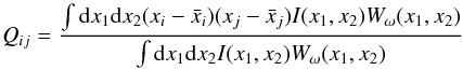${\mathit{Q}}_{\mathit{ij}}\mathrm{=}\frac{\mathrm{\int }\mathrm{d}{\mathit{x}}_{\mathrm{1}}\mathrm{d}{\mathit{x}}_{\mathrm{2}}\mathrm{(}{\mathit{x}}_{\mathit{i}}\mathrm{-}\mathit{x̅}\mathit{i}\mathrm{)}\mathrm{(}{\mathit{x}}_{\mathit{j}}\mathrm{-}\mathit{x̅}\mathit{j}\mathrm{)}\mathit{I}\mathrm{\left(}{\mathit{x}}_{\mathrm{1}}\mathit{,}{\mathit{x}}_{\mathrm{2}}\mathrm{\right)}{\mathit{W}}_{\mathit{\omega }}\mathrm{\left(}{\mathit{x}}_{\mathrm{1}}\mathit{,}{\mathit{x}}_{\mathrm{2}}\mathrm{\right)}}{\mathrm{\int }\mathrm{d}{\mathit{x}}_{\mathrm{1}}\mathrm{d}{\mathit{x}}_{\mathrm{2}}\mathit{I}\mathrm{\left(}{\mathit{x}}_{\mathrm{1}}\mathit{,}{\mathit{x}}_{\mathrm{2}}\mathrm{\right)}{\mathit{W}}_{\mathit{\omega }}\mathrm{\left(}{\mathit{x}}_{\mathrm{1}}\mathit{,}{\mathit{x}}_{\mathrm{2}}\mathrm{\right)}}\hspace{0.17em}$(1)where i and j = { 1,2 }, and (x₁,x₂) is a Cartesian coordinate system. W_ω(x₁,x₂) is a weight function that is typically assumed to a be a multivariate Gaussian of scale ω. There are three quadrupole moments Q = { Q₁₁, Q₂₂, Q₁₂ } that are therefore defined, and these can be related to the ellipticity of the object in question by 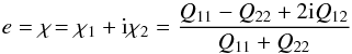$\mathit{e}\mathrm{=}\mathit{\chi }\mathrm{=}{\mathit{\chi }}_{\mathrm{1}}\mathrm{+}\mathrm{i}{\mathit{\chi }}_{\mathrm{2}}\mathrm{=}\frac{{\mathit{Q}}_{\mathrm{11}}\mathrm{-}{\mathit{Q}}_{\mathrm{22}}\mathrm{+}\mathrm{2}\mathrm{i}{\mathit{Q}}_{\mathrm{12}}}{{\mathit{Q}}_{\mathrm{11}}\mathrm{+}{\mathit{Q}}_{\mathrm{22}}}\hspace{0.17em}$(2)the third eccentricity. Its denominator, $\mathit{A}\mathrm{=}{\mathit{Q}}_{\mathrm{11}}\mathrm{+}{\mathit{Q}}_{\mathrm{22}}\hspace{0.17em}$(3)measures the size of an object (referred to as R² in other works). As Fig. 1 showing how negative values of A can be measured in real data illustrates, the R² nomenclature, which sounds positive definite, appears to be more appropriate for the alternative estimator ${\mathit{A}}^{\mathrm{\prime }}\mathrm{=}\mathrm{(}{\mathit{Q}}_{\mathrm{11}}^{\mathrm{\prime }\mathrm{2}}\mathrm{+}{\mathit{Q}}_{\mathrm{22}}^{\mathrm{\prime }\mathrm{2}}\mathrm{)}\mathit{/}{\mathit{F}}^{\mathrm{2}}$, with ${\mathit{Q}}_{\mathit{ij}}^{\mathrm{\prime }}$ the numerator of Eq. (1), and F its denominator. However we note the oddity that A′ is in units of angle to the fourth power. While A, in units of angle squared, can be understood as the solid angle subtended by the object, there is no similarly straightforward interpretation for A′. Although other definitions, for example, $\sqrt{\mathrm{(}{\mathit{Q}}_{\mathrm{11}}{\mathit{Q}}_{\mathrm{22}}\mathrm{-}{\mathit{Q}}_{\mathrm{12}}^{\mathrm{2}}\mathrm{)}}$ yield positive definite size estimators, we restrict our discussion to Q₁₁ + Q₂₂, because of its relevance as the denominator of χ, as we will demonstrate. In the presence of a point spread function (PSF) and detector effects the observed size and ellipticity transform as (see Appendix A and Bartelmann & Schneider 2001) ${\mathit{e}}_{\mathrm{obs}}\mathrm{\equiv }{\mathit{e}}_{\mathrm{gal}}\mathrm{+}\frac{{\mathit{A}}_{\mathrm{PSF}}}{{\mathit{A}}_{\mathrm{gal}}\mathrm{+}{\mathit{A}}_{\mathrm{PSF}}}\mathrm{(}{\mathit{e}}_{\mathrm{PSF}}\mathrm{-}{\mathit{e}}_{\mathrm{gal}}\mathrm{)}\mathrm{+}{\mathit{e}}_{\mathrm{NC}}\hspace{0.17em}$(4)and ${\mathit{A}}_{\mathrm{obs}}\mathrm{\equiv }{\mathit{A}}_{\mathrm{gal}}\mathrm{+}{\mathit{A}}_{\mathrm{PSF}}\mathrm{+}{\mathit{A}}_{\mathrm{NC}}\hspace{0.17em}$(5)where “PSF” refers to any convolutive effect and “NC” refers to any non-convolutive effect (for example due to CTI), “obs” refers to the observed quantity and “gal” denotes the (true) galaxy quantity that would be observed given no additional effects. Equations (4) and (5) correct Eqs. (31) and (32) of Massey et al. (2013, M13), and we detail the subsequent changes to the requirement flowdown model in Appendix A.

Cosmic shear analyses typically involve calculating correlations between galaxy shapes by taking the two-point correlation function of Eq. (4), and in taking the ensemble average (mean) of the derived expressions, requirements can be determined on each the convolutive and non-convolutive elements of an experiment design. This leads to expressions like ⟨ δA/A ⟩, where δ refers to a measurement uncertainty, upon which there is a requirement. This is particularly important for the non-convolutive effects where there are requirements that depend on quantities such as ⟨ δA_NC/A_obs ⟩ (M13; Cropper et al. 2013).

Because the quadrupole moments are sums over pixels, they are expected (through the central limit theorem) to be Gaussian distributed. Derived quantities that are linear combinations of the quadrupole moments, such as numerator and denominator (the size A) in Eq. (2), are also Gaussian distributed. However it is by taking the ratio in Eq. (2) that χ follows a distribution whose mean and variance formally and practically diverge. We note that χ will diverge for a general distribution of the quadrupole moments, independent of the choice of W_ω.

In the cosmic shear requirement flowdown (M13), it is the denominator in terms such as ⟨ δA_NC/A_NC ⟩ that causes the problem: if the distribution of the denominator crosses zero then the distribution of the ratio diverges. Because the mean of the ratio of two correlated variables is undefined it is therefore not formally possible to verify if quantities such as ⟨ δA_NC/A_obs ⟩ are being measured correctly – one can make the approximation ⟨ δA_NC ⟩ / ⟨ A_obs ⟩ but then it is not possible to verify that this is a sufficient approximation.

2.2. Why objects with negative sizes A exist

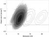Fig. 1 Histogram of the measured values of Aobs = Q11 + Q22 from simulations of the CTI effect, as a function of the object signal-to-noise ratio. The logarithmic grey scale and white contours (enclosing 68.3%, 95.45%, and 99.73% of samples, respectively) show the 107 exponential disk galaxies analysed in I15. Input simulations containing Poisson distributed sky noise were subjected to CTI and Gaussian read-out noise. Then, the CTI was removed using the correct trap model. Dashed and dot-dashed contours (both smoothed) enclose the same density levels measured from 105 simulations with ~35% (~85%) higher signal-to-noise. In all three cases, the noise causes a non-negligible fraction of the galaxies to be measured with Aobs< 0.

Let us revisit the size measurement of simulated galaxies in I15, and analyse the role and impact of very small objects. Galaxies of negative measured size A_obs are problematic for two related reasons: as we have just seen, they make terms with the size in the denominator diverge (recall that A_obs itself is Gaussian distributed). Moreover, because the distribution of A_obs extends to negative values the Marsaglia (2006) mitigation technique (cf. Appendix B) cannot be applied to measure ellipticity statistics. From where do A_obs ≤ 0 sources arise?

In general, a measured Q_ij can be negative if an image is noisy. Consider the case that there is a local background M(x₁,x₂), with mean ⟨ M ⟩ and noise about this mean, then we measure in the presence of this background $\begin{array}{c}\mathrm{˜}\\ {\mathit{Q}}_{\mathrm{11}}\end{array}\mathrm{=}\mathrm{\int }\mathrm{\left[}\mathit{I}\mathrm{\right(}{\mathit{x}}_{\mathrm{1}}\mathit{,}{\mathit{x}}_{\mathrm{2}}\mathrm{)}\mathrm{+}\mathit{M}\mathrm{(}{\mathit{x}}_{\mathrm{1}}\mathit{,}{\mathit{x}}_{\mathrm{2}}\mathrm{\left)}\mathrm{\right]}\hspace{0.17em}{\mathit{W}}_{\mathit{\omega }}\mathrm{\left(}{\mathit{x}}_{\mathrm{1}}\mathit{,}{\mathit{x}}_{\mathrm{2}}\mathrm{\right)}\hspace{0.17em}{\mathit{x}}^{\mathrm{2}}\hspace{0.17em}\mathrm{d}{\mathit{x}}_{\mathrm{1}}\mathrm{d}{\mathit{x}}_{\mathrm{2}}\mathit{,}$(6)where I(x₁,x₂) is the galaxy intensity. To obtain the galaxy’s shape moments we would have to subtract the mean local moment ${\mathit{Q}}_{\mathrm{11}}\mathrm{=}\begin{array}{c}\mathrm{˜}\\ {\mathit{Q}}_{\mathrm{11}}\end{array}\mathrm{-}\mathrm{\int }\mathit{M}\mathrm{\left(}{\mathit{x}}_{\mathrm{1}}\mathit{,}{\mathit{x}}_{\mathrm{2}}\mathrm{\right)}\hspace{0.17em}{\mathit{x}}^{\mathrm{2}}\hspace{0.17em}\mathrm{d}{\mathit{x}}_{\mathrm{1}}\mathrm{d}{\mathit{x}}_{\mathrm{2}}\mathit{,}$(7)which can be zero or less then zero depending on how noisy the image and background is. In Eq. (7), the weight function W_ω(x₁,x₂) drops out because ⟨ M ⟩ is constant over object scales. In practice the mean background is usually subtracted leaving “negative” pixels in the data in a process referred to as “background subtraction”. Therefore A = Q₁₁ + Q₂₂ can be negative in practice.

Figure 1 shows an example from I15 of the distribution of measured sizes A_obs, as a function of SExtractor (Bertin & Arnouts 1996) signal-to-noise (S/N) ratio. The Rhodes et al. (2001, RRG) shape-measurement algorithm used here subtracts a mean background before calculating image moments as just described. I15 applied the ArCTIC (Massey et al. 2010, 2014) algorithm for CTI correction in CTI-addition mode to each of the 10⁷ exponential disk galaxy images used in Fig. 1, and then iteratively corrected the CTI trails using the same software and trap model. For a detailed account of our input simulation, we refer to I15.

Because ArCTIC restores the input simulation (sources convolved with a Euclid visual instrument PSF plus Poisson distributed sky noise) perfectly except for read-out noise added during the emulated CCD read-out, the distribution in Fig. 1 looks very similar to that of the input simulations. That means we would have recovered a similar distribution of size and signal to noise even in the absence of CTI. But we include it here for realism (including slightly correlated background noise due to the CTI correction). We choose the CTI-corrected images because the represent what can be measured from real observations.

While the measured size A_obs and S/N are correlated, the negative size objects in Fig. 1 do not represent the very low S/N end of the distribution in either a relative or an absolute sense. Indeed, in the I15 analysis pipeline, all of them are bona fide SExtractor detections, accounting for one in 128 (0.78%) of these galaxies sampling the faintest population to be included in the Euclid cosmic shear experiments. Increasing the S/N of the input simulations by ~15% (~35%), reduces the fraction of A_obs ≤ 0 galaxies to 0.50% (0.19%), but this is a slow drop-off (cf. dashed and dot-dashed contours in Fig. 1). Even in a simulation with mean S/N ≈ 20, we still observe negative sizes for eight out of 10⁵ samples, a tiny, but not negligible fraction in a Euclid-like survey. The tail on the low-S/N side of the distribution is an artifact of the RRG algorithm’s choice of scale ω of the weight function W in Eq. (1).

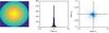Fig. 2 Example of Monte-Carlo sampling of Π(Q), with no perturbations (the fiducial case) propagated into pϵ. The left-hand panel shows the inferred prior in ϵ1 (x-axis) and ϵ2 (y-axis) calculated by taking the product of the individual ellipticity distributions. The middle panel shows the biases in ϵ1 and the right-hand panel shows the distribution of biases in ϵ1 and ϵ2. Biases are in units of arcsec2.

We note that the results shown in Fig. 1 have been calculated with a specific choice of SExtractor centroids and a Gaussian weight function (). We expect the results to depend quantitatively, but not qualitatively on these choices. In particular, the small value of ω compared to usual choices in the weak lensing literature already minimises the effect of noise on the measured moments. However, with only a few signal pixels, these sources are intrinsically vulnerable to noise.

We also note that while Fig. 1 uses the SExtractor S/N instead of a measurement based on the same moments used to compute A, this will not affect our conclusions: any two viable S/N estimators can be transformed into each other via a bijective mapping, such that, locally for the range of Fig. 1, the abscissa can be rescaled linearly into the reader’s preferred S/N estimate.

Finally, one might argue that many shape measurement algorithms employ inverse variance weights to the galaxies in their shear catalogues. Because of the large uncertainties in the resulting shear estimates, A< 0 objects will preferentially get assigned smaller weights than the average galaxy. However, unless the A< 0 galaxies are given zero weight, this will not mitigate the problem. Our simulations take into account the ensemble scatter of the estimated A = Q₁₁ + Q₂₂.

3. Methodology

Here, we present the two mitigation strategies we discuss. Sect. 3.1 describes the effect of size cuts on CTI correction as an example of the first strategy. Section 3.2 details how requirements can be recast in terms of the normally distributed quadrupole moments.

3.1. Removing negative size sources from CTI simulations

Although the A_obs ≤ 0 sources are legitimate objects for shape measurement, removing them from the catalogue by means of a size cut can solve some of the mathematical problems arising from the vanishing denominator in Eq. (2). In fact, most existing shear measurement algorithms impose a size cut at or above the size scale measured from observed PSF tracing stars, for practical purposes. However, the I15 sensitivity analysis did not consider such size cuts when translating the requirements on observables like e_obs into requirements on the accuracy and precision to which the parameters of ArCTIC, the CTI model, need to be determined by calibration. Instead, I15 maximised their sample statistics by taking into account the full distribution in A_obs.

We repeat the analysis of I15 with an increasingly selective size cut on A_obs (that is on the size of objects after CTI has been first applied and then corrected), mimicking realistic conditions. Because the Gaussian read-out noise that is added just after CTI has been applied, and is uncorrelated to the Poisson distributed sky noise in the input simulation, and ${\mathit{A}}_{\mathrm{obs}}\mathrm{=}{\mathit{A}}_{\mathrm{gal}}\mathrm{+}{\mathit{A}}_{\mathrm{PSF}}\mathrm{+}{\mathit{A}}_{\mathrm{sky}\mathrm{\_}\mathrm{noise}}\mathrm{+}{\mathit{A}}_{\mathrm{NC}}\mathrm{+}{\mathit{A}}_{\mathrm{read}\mathrm{\_}\mathrm{noise}}\mathit{,}$(8)the sources A_obs ≤ 0 only rarely coincide with the sources A_gal + A_PSF + A_{sky_noise} ≤ 0 in the input simulations. Indeed, our simulations allow us to trace that in the I15 setup and sample A_NC + A_{read_noise} are well fit by a Gaussian distribution of mean and standard deviation of (the I15 simulations used here and in Sect. 4.1 have a pixel scale of /pixel).

3.2. How to link requirements to moments

As we will see in Sect. 4.1, making size cuts in weak lensing analyses can make requirements assessment more robust. However there are also negative impacts, most notably (1) the reduction in the number of galaxies; and (2) the introduction of a non-trivial relationship between the size cut, CTI correction, signal-to-noise, and the shape measurement method employed (Sect. 4.1.2). Thus we explore an alternative mitigation strategy.

In this approach we propose that instead of setting requirements on the ellipticity and size, requirements need to be set in the quadrupole moment space. We still propose that ellipticities are used for shear inference (using the quadrupole moments themselves is explored in Viola et al. 2014), and that only the requirements are set in the moment space.

The requirements we will set are on the accuracy with which the true distribution of moments needs to be known (that would have been observed in the absence of any systematic biases, in other words, the prior distribution of the quadrupole moments). We therefore start by measuring this distribution, about which perturbations can be made. To get a realistic fiducial baseline we measure this from data using the GalSim (Mandelbaum et al. 2012; Rowe et al. 2015) deconvolved sample of galaxies (we use all galaxies in this sample; for a full description of the magnitude range and other properties we refer to the GalSim papers), where we use a weight function for the moments that is an multivariate Gaussian with a FWHM of 20 pixels (the pixel scale is 0.2 arcsec); we find that the results are independent of the exact choice of this width since we take perturbations about the fiducial distribution. Throughout units of the quadrupole moments are in arcseconds squared unless otherwise stated.

Viola et al. (2014) show how a given measured set of quadrupole moment values Q and their measurement errors σ_Q relate to a probability distribution for ellipticity p_χ. This is known as the “Marsaglia-Tin” distribution (Marsaglia 1965, 2006; Tin 1965) and is the multivariate correlated case of the ratio distribution. The mean and maximum likelihood of the ellipticity probability distributions are biased, in a way that is dependent on the measured error on the quadrupole moments (or signal-to-noise of the observed galaxy image).

We define a measured quadrupole distribution p_i(Q) for a galaxy i. In a Bayesian setting the distribution of the true quadrupole moments can be considered as a prior Π(Q) from which the galaxy is drawn. That means the probability of measuring a value Q given some data D can be written like p_i(Q | D) ∝ p(D | Q)Π(Q). The distribution p_i(Q) can then be mapped into ellipticity via the Marsaglia-Tin distribution, arriving at the biases in the mean of the elliptcity components.

Doing so, it is advantageous to use here the third flatterning, an alternative ellipticity estimator 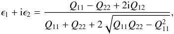${\mathit{ϵ}}_{\mathrm{1}}\mathrm{+}\mathrm{i}{\mathit{ϵ}}_{\mathrm{2}}\mathrm{=}\frac{{\mathit{Q}}_{\mathrm{11}}\mathrm{-}{\mathit{Q}}_{\mathrm{22}}\mathrm{+}\mathrm{2}\mathrm{i}{\mathit{Q}}_{\mathrm{12}}}{{\mathit{Q}}_{\mathrm{11}}\mathrm{+}{\mathit{Q}}_{\mathrm{22}}\mathrm{+}\mathrm{2}\sqrt{{\mathit{Q}}_{\mathrm{11}}{\mathit{Q}}_{\mathrm{22}}\mathrm{-}{\mathit{Q}}_{\mathrm{11}}^{\mathrm{2}}}}\mathit{,}$(9)that relates to χ as χ = 2ϵ/ (1 + | ϵ | ²). We choose to transform to ϵ here instead of χ, because the range of ϵ is the unit disk, while χ has an infinite range (cf. Fig. 1 of Viola et al. 2014). Thus, a ϵ allows us to sample extremely elliptical objects in an unbiased way, leading to well-defined moments for p_ϵ. Moreover, we explicitly take into account the correlation between the moments, in particular also between numerator and denominator of χ.

We will place requirements on how well the mean and error of the moment distribution needs to be known in order to ensure small biases on ellipticity. The procedure we take is as follows. We perform Monte-Carlo sampling from the Π(Q) distribution, for each sampled value we assign a measurement error equal to the value given above to define a p_i(Q) (σ(Q₁₁) = 0.020, σ(Q₂₂) = 0.019, σ(Q₁₂) = 0.012, all in arcsec²). We then transform this to p_ϵ,i and compute the bias in the mean of this distribution away from the values computed by using the mean values μ(Q_ij) in Eq. (9); the bias is the difference between the two. This results in a distribution of biases in ϵ₁ and ϵ₂ from which a mean bias ⟨ bias ϵ_i ⟩, and error on the bias σ(ϵ_i), can be computed. We perform this for the fiducial distribution and then repeat the process for distributions Π(Q) for which the mean and error have been perturbed. We can then compute the relative change in the biases caused by the perturbations b_e( { Q_F } )−b_e( { Q_F + δQ }) (where b_e are biases in ellipticity that are a function of a fiducial set of moments { Q_F } and perturbations about these { Q_F + δQ }), and therefore relate the knowledge of this distribution to biases in ellipticity. We assume that given a well-defined measurement of the moments the fiducial bias can be corrected for using the analytic results from the Marsaglia-Tin distribution.

We note that the process allows one to place requirements on the quadrupole moments, that ensure unbiased ellipticity measurements, with avoiding the need to estimate any ratios of variables. The ellipticities thus derived are therefore usable in an unbiased way for cosmological parameter inference following the formalisms followed in Amara & Réfrégier (2008), Kitching et al. (2009) and M13.

In Fig. 2 we show an example of the process. We present 1000 Monte-Carlo realisations of the fiducial Π(Q) distribution propagated into p_ϵ. We show the product of the ellipticity distributions ${}^{\mathrm{􏽑}}\mathit{p}_{\mathit{ϵ,i}}$, which returns the inferred prior (the intrinsic ellipticity) distribution (as shown in Miller et al. 2007) and the distribution of biases in ϵ₁ and ϵ₂ as a result of taking realisations from the Π(Q) distribution.

4. Results

4.1. Results for the size cut method

4.1.1. Size cuts and CTI correction sensitivity

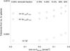Fig. 3 Relative tolerances for changes in ArCTIC trap model parameters based on the Euclid requirement for Δe1 in galaxies, as a function of the minimum observed size Aobs,min included in the analysis. Larger tolerances mean less strict calibration requirements. We show results for the well fill power β, and the densities ρ1,2,3 and release time-scales τ1,2,3 of all trap species considered by I15 (cf. their Table 3).

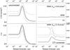Fig. 4 CTI-induced relative size bias ΔA/A (upper panels) and ellipticity bias Δe1 (lower panels) caused by a single trap species of time scale τ (in units of pixels clocked charge has travelled) and unit density. Measurements before (left panels) and after (right panels) CTI correction are shown for the I15 faint galaxy sample for four shape measurement choices: the I15 default (iterative centroiding and adaptive weight function width ω and ; grey solid lines; also cf. Fig. 2 of I15); the most shape-measurement independent (MSMI) choice of SExtractor centroids and fixed (black solid lines); MSMI with a size cut (dashed lines) and MSMI with a size cut (dot-dashed lines, off scale for ΔA/A). Uncertainties are smaller than the line widths. The results in this figure correspond to a trap density of 24% of the Euclid end-of-life estimate.

Re-creating the results of I15 with different size cuts A_obs,min in place, we find the effect of a size cut on the CTI correction sensitivity, that is the required precision to which the ArCTIC parameters need to calibrated, to be reassuringly small. To first order, and especially so for size cuts A_obs,min affecting only the extreme tail of the distribution, CTI correction works independent of a size cut. After all, we deal with a pixel-level correction before the extraction of a catalogue.

Figure 3 presents the tolerances (bias margins) for the parameters I15 found to yield the tightest margins given the Euclid requirement on CTI-induced ellipticity bias ∆e₁ = 〈e_1,corrected〉−〈e_1,input 〉 , as a function of a size cut A_obs>A_obs,min. We only consider CTI along the x₁ axis. We probe the densities ρ and release time-scales τ of the trap species. The same relative biases in ρ_i and τ_i are tested simultaneously for all three trap species in the I15 baseline model. We also probe the well fill power β describing the volume growth of a charge cloud inside a pixel as a function of number of electrons. We derive tolerances on the deviation of the parameters from the fiducial values by fitting to the measured Δe₁(Δβ) and the other parameters in the same way as I15. Thus, without a size cut (leftmost points in Fig. 3), we reproduce the tolerances given in Table 3 of I15.

We observe a significant change in tolerances only for size cuts removing at least several per cent of the catalogue sources. Moreover, the size cuts act in a way that render Δe₁ more robust to biases in the trap parameters. This is what we expect when removing objects with a denominator in Eq. (2) close to zero, while slightly increasing the average S/N. A size cut at the scale of the PSF size would have the welcome side-effect of widening the margins in the crucial ArCTIC parameters by ~70%.

4.1.2. Disentangling CTI correction and shape measurement

Any size cut, however, affects what I15 termed the CTI correction zeropoint, that is the residual bias due to overcorrected read-out noise that is present even if the ArCTIC parameters are perfectly known and correct. (Consistent with I15, we tacitly assumed this effect to be absent in the analysis leading to Fig. 3. Indeed, the zeropoint can be calibrated out of real data at the catalogue stage.) This is obvious for the zeropoint in ∆A = ⟨A_corrected⟩−⟨A_input⟩ ≡ ⟨A_obs⟩−⟨A_input⟩ . Removing objects below a threshold in A_obs increases ⟨ A_obs ⟩, but leaves ⟨ A_input ⟩ unchanged, as we saw in Sect. 4.1.1.

While we observe the expected monotonic increase in the ΔA zeropoint, the zeropoint CTI bias in e₁ (with A in the denominator) shows a more complicated, non-monotonic behaviour as a function of A_obs,min.

Moreover, analysing simulations with a variable amount of read-out noise, we also find a non-monotonic dependency of the Δe₁ zeropoint, instead of the increasing (in absolute terms) CTI correction residuals illustrated in Fig. 3 of I15. Because adding more noise between applying CTI and correcting cannot lead to a better reconstruction of the true, underlying pre-CTI image, these findings are best explained by an artifact of the (simple) shear measurement pipeline we are using. SExtractor catalogues are fed into the RRG algorithm which iteratively determines a centroid and, in the I15 setup, calculates the size (standard deviation) of the Gaussian weight function in Eq. (1) as $\mathit{\omega }\mathrm{=}\mathrm{2}\sqrt{\mathrm{\Omega }\mathit{/}\mathit{\pi }}$, with Ω the SExtractor area.

These steps are susceptible to the same noise fluctuations of the local background that can make A negative. Because our goal is to allocate uncertainty margins to each element of the Euclid cosmic shear experiment, and validate algorithms against these requirements, we seek to disentangle effects of shape measurement and CTI correction. We thus propose a “most shape measurement independent” (MSMI) measurement of the CTI-induced biases in galaxy morphometry, and compare to I15 to gauge the magnitude of pipeline effects on CTI correction.

Our MSMI setting directly uses SExtractor centroids for the galaxies, switching off the iterative refinement. We fix the weight function size to a fixed, small value of , to minimise the effect of outlying sky pixels. Our value matches the sample average of ω I15 recorded for the same galaxies.

Figure 4 shows the CTI-induced ΔA/A (upper panels) and Δe₁ (lower panels) arising from a single trap species of time scale τ before (left panels) and after (right panels) CTI correction. Qualitatively, the MSMI (black lines) and I15 (grey lines; see also their Fig. 2) are in broad agreement, with the traps causing the strongest biases slightly shifting towards longer release times τ. Possibly this is due to more objects being slightly off-centred in the more simplistic MSMI setup, and thus more sensitive to their electrons being dragged out of the aperture.

After CTI correction, the MSMI measurements return a significantly smaller residual ΔA/A than the I15 settings over the whole eight decades in release time τ we tested. Curiously, the I15 pipeline performs better in residual Δe₁ for a random τ, but our reducing the influence of the shape-measurement pipeline nulls away the zeropoint bias of the most effective charge traps at the peak of the curve.

We also introduce size cuts in the MSMI measurements (dashed and dot-dashed lines in Fig. 4). These size cuts lower the bias Δe₁ for all traps, likely by removing the some of the most biases sources. However, by the mechanism described in Sect. 4.1.1, size cuts introduce an additional bias in ΔA/A that the CTI correction cannot account for (but which could be removed by calibration).

A complete understanding of the interaction between the ArCTIC CTI correction, shape measurement algorithms and source selection by size cuts exceeds the scope of this paper. We conclude that they should be disentangled as far as possible and provide empirical fits to the results of Fig. 4, updating Table 1 of I15 as a baseline for further research. As I15 demonstrated, the combined effect of several trap species are linear combinations of the biases caused by their component trap species.

4.2. Results for requirements recast on quadrupole moments

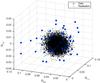Fig. 5 Distribution of the measured quadrupole moments measured in GalSim galaxies. We show only 100 points here, in blue. The black points show a set of 1000 values sampled from a multivariate Gaussian derived from the measured values. All axes are in units of arcsec2.

Figure 5 shows the measured distribution of moments Π(Q) measured in GalSim galaxies. We find that indeed the quadrupole moments are consistent with a Gaussian distribution with a mean for each component of μ(Q₁₁) = 0.042, μ(Q₂₂) = 0.039, μ(Q₁₂) = 7 × 10^-4 and an error on each component of σ(Q₁₁) = 0.020, σ(Q₂₂) = 0.019, σ(Q₁₂) = 0.012; reported in units of arcseconds squared throughout.

We also measured these values from COSMOS data (Leauthaud et al. 2007) and found values (in arcsec²) of σ(Q₁₁) = 0.09, μ(Q₁₁) ~ 0.02, σ(Q₁₂) = 0.040, μ(Q₁₂) ~ 0 before PSF correction. We repeat the analysis in Sect. 4.2 with these values, and recover the same requirements on ellipticity to four decimal places, or ~5% of the requirement.

The error on Q₁₂ is expected to be approximately σ(Q₁₂) ≈ 0.5(σ²(Q₁₁) + σ²(Q₂₂))^1/2. Through expected symmetries we assume in our analysis that μ(Q₁₂) = 0, μ(Q₁₁) = μ(Q₂₂) and σ(Q₁₁) = σ(Q₂₂). The moments are correlated as shown in Viola et al. (2014), and using these correlation coefficients we can then make random realisations of this distribution that we also show in Fig. 5.

About the fiducial quadrupole moment distribution Π(Q) we make a 1000 perturbations where we vary the mean and the errors, each a uniform random number between r = [−0.01,0.01], for example for the mean μ(Q₁₁) → μ(Q₁₁) + r, and similarly for the other variables each with an independent value. In this way we are searching the six-dimensional “requirement space” (the means and standard deviations of each moment direction) in a random way – a more sophisticated implementation could use Markov-chain optimisation for example. For each realisation of Π(Q) we sample 10⁴ points from this distribution and then follow the procedure outlined in Sect. 3.2.

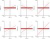Fig. 6 Dependency of the mean and error of ellipticity biases as a function of changes in the mean and error of the ensemble quadrupole moment distribution (in arcsec2). The red lines show linear fits to the distributions (grey points), and the red bar shows ±2 × 10-3 arcsec2.

In Fig. 6 we show the dependency of the mean and error of the ellipticity biases, as a function of perturbations in the mean and error on the quadrupole moment distribution. The mean and error of the bias for each ellipticity component depends on the all the six varied parameters, however there is a primary direction in this parameter space along which the strongest dependency occurs, for example the mean bias in ϵ₁ is most sensitive to changes in the mean of the Q₁₁ as is expected, so we only show these strongest dependencies. We now derive our main requirements taking only into account these dominant dependencies.

We find that there is an approximately linear dependency between the mean bias and the mean of the quadrupole moments, and between the error on the bias and the error of the quadrupole moment distribution. By taking the requirement in biases on ellipticity (e.g. from Kitching et al. 2009) of 2 × 10^-3 arcsec² we can therefore set a requirement on the moments of quadrupole moment distribution – where the bias in ellipticity exceeds the absolute value of this. We show the knowledge of mean and error of each quadrupole moment show in Table 2. As a rule of thumb we find that the error on the standard deviation of each component needs to be smaller than 1.4 × 10^-3 arcsec². Alternatively the requirement on Stokes parameters Q₁₁ + Q₂₂ and 2Q₁₂ is 1.9 × 10^-3 arcsec².

5. Implications for Euclid CTI correction

The wider uncertainty margins on CTI trap parameters found in Sect. 4 – up to 70% – underline the positive role that size cuts to the galaxy catalogue can have in shear experiments. However, we have to caution that this new result does not mean efforts on CTI calibration have become less crucial for the Euclid mission, for three reasons.

First, there will be a size cut in Euclid shear catalogue anyway, very likely at some value slightly larger than the PSF size. What has improved is our modelling of an experiment’s sensitivity to CTI, addressing an aspect that was missing in I15.

Second, the 70% improvement specifically applies to our baseline trap model, the mix of trap species defined in I15, which is informed by laboratory experiments on Euclid VIS CCDs, but should be seen as a realistic example, not a prediction of the actual Euclid CTI.

Third, we observe the CTI correction, the (simple) shape measurement pipeline we used, and the size cut on the source catalogue to interact non-trivially. We simplified the shape measurement algorithm further and find the residual size and ellipticity biases after CTI correction to decrease for many relevant charge trap species. Our results provide a new baseline for further research.

While size cuts further prevent biases that would arise if a galaxy of measured size smaller than the PSF was corrected for PSF effects, no PSF correction has been performed in either I15 or this work. This approach is justified because Euclid requirements on shape measurement are kept deliberately distinct from those on PSF knowledge and correction. Setting separate requirements on the shear numerator and denominator is also consistent with the separation of numerator and denominator (for PSF and weight function correction) in the RRG method.

When deriving these individual measurements of the surface brightness moments, we do not investigate the requirements on the covariances of the moments, taking instead the theoretical covariance estimated from Viola et al. (2014). In future work, however, these could also be investigated, and are likely to depend on the weight function used in the analysis (which could be even optimised for this purpose).

Moreover, we need to caution that while the most important quantities for which a weak lensing survey needs to set requirements can be expressed via surface brightness moments, there will be some degree of information loss inherent to the compression of the lensing map (from a two-dimensional input to a two-dimensional output) using only low-order surface brightness moments. This limitation is common to ellipticity-based and moment-based requirements.

6. Conclusions

Weak lensing is a potentially powerful probe of cosmology, but the experiments and algorithms to measure this phenomenon need to be carefully designed. To this end a series of requirements on instrumental and detector systematic effects has been previously derived based on the propagation of measured changes in ellipticity and size into changes on cosmological parameter inference. However in doing this, the relationship between ellipticity and size leads to requirements being placed on the mean of two measured random variables. Such moments are not defined in general and therefore cannot be measured, so that such requirements cannot be tested.

Especially problematic are those sources whose measured size is close to zero or negative, because estimation techniques like the Marsaglia (2006) re-parametrisation cannot be applied. However galaxies of negative measured size represent legitimate samples from the size distribution of faint, small objects in the presence of noise that still occur with non-negligible frequently at S/N ≳ 15.

Removing the smallest galaxies from source catalogues by means of a size cut is a viable strategy in many, but not all weak lensing contexts. Sampling from a clipped source distribution may introduce unwanted biases in the complex data analysis chains. We extend the I15 sensitivity study of the charge transfer inefficiency (CTI) correction to include a size cut. We find the tolerance margins in CTI correction parameters to show a moderate dependence on removing the smallest sources. In fact, uncertainty margins are found to be wider by up to ~70% in the tested set-up.

As a more robust long-term solution, we present a formalism that allows requirements on ellipticity to be set in the space of quadrupole moments, that are linear functions of the data, where no ratios need to be computed, using the probability distribution for ellipticity derived in Viola et al. (2014). We find that the mean and the error of the distribution of quadrupole moments over the ensemble of galaxies used in a Stage-IV weak lensing experiment needs known to better than 1.4 × 10^-3 arcsec² in each component for the ellipticity measurements to be unbiased at the level of 2 × 10^-3 arcsec².

This requirement can now serve as a basis from which a breakdown and proportion into individual requirement on PSF and detector effects can be made as is done in Cropper et al. (2013). This should be straightforward given the formulae provided in Melchior et al. (2010) for example. We do not perform this breakdown here as the proportioning is flexible and should be done with instrument-specific knowledge: for example one may have a very stable PSF and wish to proportion more flexibility to instrument effects or vice versa. In this study we propagate only requirements to ellipticity, and marginalise over size; however if one wishes to use weak lensing magnification as an additional cosmological probe then this could be used to set joint ellipticity and size requirements. The setting of these requirements can now serve as a firm statistical basis from which weak lensing experimental design can proceed.

Finally, we point out that because recasting the requirements does not affect the galaxy selection as the size cuts do, there is no need to update the CTI trap model sensitivity results of I15 for this case. Rather, these two elements work together: we have updated the CTI results to a more realistic model, while identifying a more appropriate way to define the requirements setting the context for the CTI correction in Euclid.

Acknowledgments

The authors would like to thank Henk Hoekstra, Peter Schneider, and Massimo Viola for helpful discussions. T.D.K. and R.M. are supported by Royal Society University Research Fellowships. The authors thank the anonymous referee for helpful suggestions. H.I. and R.M. are supported by the Science and Technology Facilities Council (grant numbers ST/H005234/1 and ST/N001494/1) and the Leverhulme Trust (grant number PLP-2011-003).

References

Appendix A: Update of M13 CTI requirements derivation

Since M13, we have found it more physical to consider non-convolutive effects like CTI as linearly affecting an object size 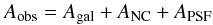${\mathit{A}}_{\mathrm{obs}}\mathrm{=}{\mathit{A}}_{\mathrm{gal}}\mathrm{+}{\mathit{A}}_{\mathrm{NC}}\mathrm{+}{\mathit{A}}_{\mathrm{PSF}}\hspace{0.17em}$(A.1)and ellipticity 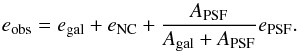${\mathit{e}}_{\mathrm{obs}}\mathrm{=}{\mathit{e}}_{\mathrm{gal}}\mathrm{+}{\mathit{e}}_{\mathrm{NC}}\mathrm{+}\frac{{\mathit{A}}_{\mathrm{PSF}}}{{\mathit{A}}_{\mathrm{gal}}\mathrm{+}{\mathit{A}}_{\mathrm{PSF}}}{\mathit{e}}_{\mathrm{PSF}}\mathit{.}$(A.2)We now derive equivalent versions of Eqs. (34) to (37) in M13, the Taylor expansion detailing the sensitivity of observables to biases in ellipticity e₁ and size A. We ignore noise terms in the following and note that Eqs. (A.1) and (A.2) only hold true to linear order in moments. Not including PSF, we have ${\mathit{e}}_{\mathrm{obs}}\mathrm{=}\frac{{\mathit{Q}}_{\mathrm{11}}\mathrm{-}{\mathit{Q}}_{\mathrm{22}}\mathrm{+}\mathrm{(}\mathit{\delta }{\mathit{Q}}_{\mathrm{11}}\mathrm{-}\mathit{\delta }{\mathit{Q}}_{\mathrm{22}}\mathrm{)}}{{\mathit{Q}}_{\mathrm{11}}\mathrm{+}{\mathit{Q}}_{\mathrm{22}}\mathrm{+}\mathrm{(}\mathit{\delta }{\mathit{Q}}_{\mathrm{11}}\mathrm{+}\mathit{\delta }{\mathit{Q}}_{\mathrm{22}}\mathrm{)}}$(A.3)where δQ are the change in moments caused by CTI. This is approximately e_obs = e_gal + e_NC if δQ ≪ Q to linear order. We note this is a further reason for using Q requirements directly. This means that: $\begin{array}{ccc}{\mathit{e}}_{\mathrm{gal}}& \mathrm{=}& \frac{\mathrm{(}{\mathit{e}}_{\mathrm{obs}}\mathrm{-}{\mathit{e}}_{\mathrm{NC}}\mathrm{)}\mathrm{(}{\mathit{A}}_{\mathrm{obs}}\mathrm{-}{\mathit{A}}_{\mathrm{NC}}\mathrm{)}\mathrm{-}{\mathit{e}}_{\mathrm{PSF}}{\mathit{A}}_{\mathrm{PSF}}}{\mathrm{(}{\mathit{A}}_{\mathrm{obs}}\mathrm{-}{\mathit{A}}_{\mathrm{NC}}\mathrm{)}}\\ & \mathrm{=}& \mathrm{(}{\mathit{e}}_{\mathrm{obs}}\mathrm{-}{\mathit{e}}_{\mathrm{NC}}\mathrm{)}\mathrm{-}\frac{{\mathit{e}}_{\mathrm{PSF}}{\mathit{A}}_{\mathrm{PSF}}}{\mathrm{(}{\mathit{A}}_{\mathrm{obs}}\mathrm{-}{\mathit{A}}_{\mathrm{NC}}\mathrm{)}}\mathit{,}\end{array}$(A.4)and consequently $\frac{\mathit{\partial }{\mathit{e}}_{\mathrm{gal}}}{\mathit{\partial }{\mathit{A}}_{\mathrm{NC}}}\mathrm{=}\mathrm{-}\frac{{\mathit{e}}_{\mathrm{PSF}}{\mathit{A}}_{\mathrm{PSF}}}{\mathrm{(}{\mathit{A}}_{\mathrm{obs}}\mathrm{-}{\mathit{A}}_{\mathrm{NC}}{\mathrm{)}}^{\mathrm{2}}}\mathit{,}$(A.5)and $\frac{\mathit{\partial }{\mathit{e}}_{\mathrm{gal}}}{\mathit{\partial }{\mathit{e}}_{\mathrm{NC}}}\mathrm{=}\mathrm{-}\mathrm{1}\hspace{0.17em}$(A.6)so that the δR_NC term in the M13 Taylor expansion (their Eq. (36)) should be replaced by $\frac{{\mathit{A}}_{\mathrm{PSF}}\hspace{0.17em}{\mathit{e}}_{\mathrm{PSF}}}{\mathrm{(}{\mathit{A}}_{\mathrm{gal}}\mathrm{+}{\mathit{A}}_{\mathrm{PSF}}{\mathrm{)}}^{\mathrm{2}}}\mathit{\delta }{\mathit{A}}_{\mathrm{NC}}\mathit{,}$(A.7)

and the δe_NC term (Eq. (37) in M13) is simply $\mathrm{-}\mathit{\delta }{\mathit{e}}_{\mathrm{NC}}\hspace{0.17em}$(A.8)this leads to a term like $⟨{\left(\frac{{\mathit{A}}_{\mathrm{PSF}}}{\mathrm{(}{\mathit{A}}_{\mathrm{gal}}\mathrm{+}{\mathit{A}}_{\mathrm{PSF}}{\mathrm{)}}^{\mathrm{2}}}\right)}^{\mathrm{2}}⟩\mathit{,}$(A.9)in the ellipticity two-point correlation function or power spectrum, which needs to be evaluated in order to check the requirement level contribution. Problems will occur in taking the ratio in the regime that A_gal + A_PSF = A_obs−A_NC → 0.

These terms make intuitive sense in that if the PSF ellipticity is zero, then any ellipticity-independent size change will not cause a bias in ellipticity. Whereas a change in ellipticity caused by CTI, that adds linearly, should cause a linear bias.

Appendix B: The Marsaglia mitigation technique

Marsaglia (2006) demonstrate that the ratio z/w of two normally distributed random variables z and w with respective means μ_z, μ_w, variances σ_z, σ_w and correlation ρ follows the same distribution as $\frac{\mathit{a}\mathrm{+}\mathit{x}}{\mathit{b}\mathrm{+}\mathit{y}}$ where x and y are uncorrelated standard normal random variables. The constants a and b are given by $\mathit{b}\mathrm{=}\frac{{\mathit{\mu }}_{\mathit{w}}}{{\mathit{\sigma }}_{\mathit{w}}}\mathit{,} \mathit{a}\mathrm{=}\mathrm{\pm }\frac{{\mathit{\mu }}_{\mathit{z}}\mathit{/}{\mathit{\sigma }}_{\mathit{z}}\mathrm{-}\mathit{\rho }{\mathit{\mu }}_{\mathit{w}}\mathit{/}{\mathit{\sigma }}_{\mathit{w}}}{\sqrt{\mathrm{1}\mathrm{-}{\mathit{\rho }}^{\mathrm{2}}}}\mathit{>}\mathrm{0.}$(B.1)Although no formal proof is given, Marsaglia (2006) show that, for practical purposes, the mean and variance of the ratio exist and are approximated by $\mathit{\mu }\mathrm{=}\frac{\mathit{a}}{\mathrm{1.01}\mathit{b}\mathrm{-}\mathrm{0.2713}}\mathit{,} \mathit{\sigma }\mathrm{=}\frac{{\mathit{a}}^{\mathrm{2}}\mathrm{+}\mathrm{1}}{{\mathit{b}}^{\mathrm{2}}\mathrm{+}\mathrm{0.108}\mathit{b}\mathrm{-}\mathrm{3.795}\mathrm{-}{\mathit{\mu }}^{\mathrm{2}}}\mathit{,}$(B.2)as long as the conditions b> 4 and a< 2.5 are satisfied. In other words, negative samples must only occur very rarely (as 4σ events or scarcer) for the Marsaglia mitigation technique to be applicable. Figure 1 shows that this condition is not met for typical faint weak lensing test galaxies.

All Tables

All Figures

Fig. 1 Histogram of the measured values of Aobs = Q11 + Q22 from simulations of the CTI effect, as a function of the object signal-to-noise ratio. The logarithmic grey scale and white contours (enclosing 68.3%, 95.45%, and 99.73% of samples, respectively) show the 107 exponential disk galaxies analysed in I15. Input simulations containing Poisson distributed sky noise were subjected to CTI and Gaussian read-out noise. Then, the CTI was removed using the correct trap model. Dashed and dot-dashed contours (both smoothed) enclose the same density levels measured from 105 simulations with ~35% (~85%) higher signal-to-noise. In all three cases, the noise causes a non-negligible fraction of the galaxies to be measured with Aobs< 0.

In the text

Fig. 2 Example of Monte-Carlo sampling of Π(Q), with no perturbations (the fiducial case) propagated into pϵ. The left-hand panel shows the inferred prior in ϵ1 (x-axis) and ϵ2 (y-axis) calculated by taking the product of the individual ellipticity distributions. The middle panel shows the biases in ϵ1 and the right-hand panel shows the distribution of biases in ϵ1 and ϵ2. Biases are in units of arcsec2.

In the text

Fig. 3 Relative tolerances for changes in ArCTIC trap model parameters based on the Euclid requirement for Δe1 in galaxies, as a function of the minimum observed size Aobs,min included in the analysis. Larger tolerances mean less strict calibration requirements. We show results for the well fill power β, and the densities ρ1,2,3 and release time-scales τ1,2,3 of all trap species considered by I15 (cf. their Table 3).

In the text

Fig. 4 CTI-induced relative size bias ΔA/A (upper panels) and ellipticity bias Δe1 (lower panels) caused by a single trap species of time scale τ (in units of pixels clocked charge has travelled) and unit density. Measurements before (left panels) and after (right panels) CTI correction are shown for the I15 faint galaxy sample for four shape measurement choices: the I15 default (iterative centroiding and adaptive weight function width ω and ; grey solid lines; also cf. Fig. 2 of I15); the most shape-measurement independent (MSMI) choice of SExtractor centroids and fixed (black solid lines); MSMI with a size cut (dashed lines) and MSMI with a size cut (dot-dashed lines, off scale for ΔA/A). Uncertainties are smaller than the line widths. The results in this figure correspond to a trap density of 24% of the Euclid end-of-life estimate.

In the text

	Fig. 5 Distribution of the measured quadrupole moments measured in GalSim galaxies. We show only 100 points here, in blue. The black points show a set of 1000 values sampled from a multivariate Gaussian derived from the measured values. All axes are in units of arcsec2.
In the text

	Fig. 6 Dependency of the mean and error of ellipticity biases as a function of changes in the mean and error of the ensemble quadrupole moment distribution (in arcsec2). The red lines show linear fits to the distributions (grey points), and the red bar shows ±2 × 10-3 arcsec2.
In the text

References

- Amara, A., & Réfrégier, A. 2008, MNRAS, 391, 228 [NASA ADS] [CrossRef] [Google Scholar]
- Antonik, M. L., Bacon, D. J., Bridle, S., et al. 2013, MNRAS, 431, 3291 [NASA ADS] [CrossRef] [Google Scholar]
- Applegate, D. E., von der Linden, A., Kelly, P. L., et al. 2014, MNRAS, 439, 48 [NASA ADS] [CrossRef] [Google Scholar]
- Bartelmann, M., & Schneider, P. 2001, Phys. Rep., 340, 291 [NASA ADS] [CrossRef] [Google Scholar]
- Bertin, E., & Arnouts, S. 1996, A&AS, 117, 393 [NASA ADS] [CrossRef] [EDP Sciences] [Google Scholar]
- Chang, C., Jarvis, M., Jain, B., et al. 2013a, MNRAS, 434, 2121 [NASA ADS] [CrossRef] [Google Scholar]
- Chang, C., Kahn, S. M., Jernigan, J. G., et al. 2013b, MNRAS, 428, 2695 [NASA ADS] [CrossRef] [Google Scholar]
- Cropper, M., Hoekstra, H., Kitching, T., et al. 2013, MNRAS, 431, 3103 [NASA ADS] [CrossRef] [Google Scholar]
- Erben, T., Van Waerbeke, L., Bertin, E., Mellier, Y., & Schneider, P. 2001, A&A, 366, 717 [NASA ADS] [CrossRef] [EDP Sciences] [Google Scholar]
- Hinkley, D. V. 1969, Biometrika, 56, 635 [CrossRef] [MathSciNet] [Google Scholar]
- Hoekstra, H. 2007, MNRAS, 379, 317 [NASA ADS] [CrossRef] [Google Scholar]
- Huterer, D., & White, M. 2002, ApJ, 578, L95 [NASA ADS] [CrossRef] [Google Scholar]
- Israel, H., Erben, T., Reiprich, T. H., et al. 2010, A&A, 520, A58 [NASA ADS] [CrossRef] [EDP Sciences] [Google Scholar]
- Israel, H., Massey, R., Prod’homme, T., et al. 2015, MNRAS, 453, 561 [NASA ADS] [CrossRef] [Google Scholar]
- Jarvis, M., Sheldon, E., Zuntz, J., et al. 2016, MNRAS, 460, 2245 [NASA ADS] [CrossRef] [Google Scholar]
- Kaiser, N., Squires, G., & Broadhurst, T. 1995, ApJ, 449, 460 [NASA ADS] [CrossRef] [Google Scholar]
- Kitching, T. D., Amara, A., Abdalla, F. B., Joachimi, B., & Refregier, A. 2009, MNRAS, 399, 2107 [NASA ADS] [CrossRef] [Google Scholar]
- Laureijs, R., Amiaux, J., Arduini, S., et al. 2011, ArXiv e-print [arXiv:1110.3193] [Google Scholar]
- Leauthaud, A., Massey, R., Kneib, J.-P., et al. 2007, ApJS, 172, 219 [NASA ADS] [CrossRef] [Google Scholar]
- Mandelbaum, R., Hirata, C. M., Leauthaud, A., Massey, R. J., & Rhodes, J. 2012, MNRAS, 420, 1518 [NASA ADS] [CrossRef] [Google Scholar]
- Marsaglia, G. 1965, J. Am. Stat. Assoc., 60, 193 [CrossRef] [Google Scholar]
- Marsaglia, G. 2006, J. Stat. Software, 16, 1 [CrossRef] [Google Scholar]
- Massey, R., Stoughton, C., Leauthaud, A., et al. 2010, MNRAS, 401, 371 [NASA ADS] [CrossRef] [Google Scholar]
- Massey, R., Hoekstra, H., Kitching, T., et al. 2013, MNRAS, 429, 661 [Google Scholar]
- Massey, R., Schrabback, T., Cordes, O., et al. 2014, MNRAS, 439, 887 [NASA ADS] [CrossRef] [Google Scholar]
- Melchior, P., Böhnert, A., Lombardi, M., & Bartelmann, M. 2010, A&A, 510, A75 [NASA ADS] [CrossRef] [EDP Sciences] [Google Scholar]
- Melchior, P., Viola, M., Schäfer, B. M., & Bartelmann, M. 2011, MNRAS, 412, 1552 [NASA ADS] [CrossRef] [Google Scholar]
- Miller, L., Kitching, T. D., Heymans, C., Heavens, A. F., & van Waerbeke, L. 2007, MNRAS, 382, 315 [NASA ADS] [CrossRef] [Google Scholar]
- Miller, L., Heymans, C., Kitching, T. D., et al. 2013, MNRAS, 429, 2858 [Google Scholar]
- Okabe, N., & Umetsu, K. 2008, PASJ, 60, 345 [NASA ADS] [Google Scholar]
- Paulin-Henriksson, S., Amara, A., Voigt, L., Refregier, A., & Bridle, S. L. 2008, A&A, 484, 67 [Google Scholar]
- Refregier, A., Kacprzak, T., Amara, A., Bridle, S., & Rowe, B. 2012, MNRAS, 425, 1951 [NASA ADS] [CrossRef] [Google Scholar]
- Rhodes, J., Réfrégier, A., & Groth, E. J. 2001, ApJ, 552, L85 [NASA ADS] [CrossRef] [Google Scholar]
- Rowe, B. T. P., Jarvis, M., Mandelbaum, R., et al. 2015, Astron. Comput., 10, 121 [NASA ADS] [CrossRef] [Google Scholar]
- Sheldon, E. S. 2014, MNRAS, 444, L25 [NASA ADS] [CrossRef] [Google Scholar]
- Tin, M. 1965, J. Am. Stat. Assoc., 60, 294 [CrossRef] [Google Scholar]
- Viola, M., Kitching, T. D., & Joachimi, B. 2014, MNRAS, 439, 1909 [NASA ADS] [CrossRef] [Google Scholar]
- Zuntz, J., Kacprzak, T., Voigt, L., et al. 2013, MNRAS, 434, 1604 [NASA ADS] [CrossRef] [Google Scholar]