| Issue |
A&A
Volume 597, January 2017
|
|
|---|---|---|
| Article Number | A113 | |
| Number of page(s) | 9 | |
| Section | Planets and planetary systems | |
| DOI | https://doi.org/10.1051/0004-6361/201629699 | |
| Published online | 12 January 2017 | |
Discovery of the secondary eclipse of HAT-P-11 b
Hamburger Sternwarte, Universität Hamburg, Gojenbergsweg 112, 21029 Hamburg, Germany
e-mail: This email address is being protected from spambots. You need JavaScript enabled to view it.
Received: 12 September 2016
Accepted: 27 October 2016
Abstract
We report the detection of the secondary eclipse of HAT-P-11 b, a Neptune-sized planet orbiting an active K4 dwarf. Using all available short-cadence data of the Kepler mission, we derive refined planetary ephemeris increasing their precision by more than an order of magnitude. Our simultaneous primary and secondary transit modeling results in improved transit and orbital parameters. In particular, the precise timing of the secondary eclipse allows to pin down the orbital eccentricity to 0.26459-0.00048+0.00069. The secondary eclipse depth of 6.09-1.11+1.12 ppm corresponds to a 5.5σ detection and results in a geometric albedo of 0.39 ± 0.07 for HAT-P-11 b, close to Neptune’s value, which may indicate further resemblances between these two bodies. Due to the substantial orbital eccentricity, the planetary equilibrium temperature is expected to change significantly with orbital position and ought to vary between 630 K and 950 K, depending on the details of heat redistribution in the atmosphere of HAT-P-11 b.
Key words: planetary systems / stars: individual: HAT-P-11 / techniques: photometric / methods: data analysis
© ESO, 2017
1. Introduction
The extrasolar planet HAT-P-11 b (also known as KOI-3.01 and Kepler-3 b) is a super-Neptune orbiting an active K4 dwarf with a period of 4.89 days. It was discovered through the transit method by Bakos et al. (2010), using ground-based photometry in the context of the HAT project (Bakos et al. 2002, 2004). In combination with radial velocity (RV) measurements, Bakos et al. (2010) derived the orbital and planetary parameters and found that HAT-P-11 b is on a rather eccentric orbit. Using RV measurements obtained with HIRES (Vogt et al. 1994), Winn et al. (2010) confirmed the eccentric orbit and refined the orbital parameters of HAT-P-11 b. Using the Rossiter-McLaughlin effect (Rossiter 1924; McLaughlin 1924), Winn et al. (2010) conclude that the planetary orbit is highly inclined and that the planet crosses the stellar disk almost parallel to the sky-projected stellar rotation axis, a result later confirmed by Hirano et al. (2011) with independent RV measurements.
HAT-P-11 b was also observed by the Kepler mission (Borucki et al. 2010). Deming et al. (2011) analyzed the Kepler light curve of quarters 0 to 2 along with ground-based photometry and present updated transit ephemeris and planetary parameters. The host-star HAT-P-11 is highly active, showing strong rotational modulation attributable to starspots, from which a stellar rotation period of about 29 d has been inferred (Bakos et al. 2010); the potentially integer ratio of 6:1 between the stellar rotation and the planetary orbital period of HAT-P-11 b has nurtured quite a bit of discussion on star-planet interactions in the system (Béky et al. 2014). In addition to rotational modulation, prominent starspot-crossing signatures are clearly visible in the majority of Kepler transit light curves. These features were discussed by several authors including Deming et al. (2011) and Béky et al. (2014). Sanchis-Ojeda & Winn (2011) present an in-depth analysis of the spot-crossing features in 26Kepler transits and conclude that the repetitive appearance of spot-occultations in similar locations in the transit profiles confirms the misalignment of the system and indicates active latitudes on the star.
A number of attempts to detect the secondary eclipse of HAT-P-11 b using the Kepler photometry have been made (e.g., Southworth 2011; Angerhausen et al. 2015), yet a secondary eclipse was not detected, and the same applies to the case of the planetary phase curve (Angerhausen et al. 2015). While Deming et al. (2011) mention the existence of Spitzer observations of the secondary eclipse, neither a detailed analysis nor a detection has been published so far in the refereed literature.
Kepler stopped observing HAT-P-11 b in 2013 after obtaining 15 quarters or more than four years of data. In this paper we analyze the entire body of Kepler photometry of HAT-P-11 b, comprising more than two hundred primary transits, derive precise ephemeris and primary transit parameters, and ultimately detect the secondary eclipse signature.
2. Data analysis
2.1. Primary transit ephemeris
The orbital parameters of HAT-P-11 b have been determined by several authors based on different data sets (Bakos et al. 2010; Winn et al. 2010; Sanchis-Ojeda & Winn 2011). Since by now 15 quarters of space-based Kepler photometry are available, of which only a fraction has previously been used to derive ephemeris and transit parameters, we first determine updated values based on the entire available data set of Kepler.
We specifically use the data from those 14 quarters for which short-cadence photometry is available, which are quarters 0, 1, 2, 3, 4, 5, 6, 9, 10, 12, 13, 14, 16, and 17. These data cover a total of 222 primary transits. For quarter 8 only long-cadence data are available, which are not considered, because the 14 additional transits in that quarter do not significantly improve our results, and further, deformations caused by spot-crossing events are much harder to identify in long-cadence data, which makes it more difficult to account for them in the analysis. For the quarters 7, 11, and 15 no observations of HAT-P-11 are available in the MAST archive.
Our analysis is based on the simple aperture photometry (SAP) provided by the Kepler pipeline reduction from which we removed all data points flagged as invalid or bad by the pipeline. Of the 222 primary transits observed in short-cadence mode, we exclude 16 transits from our analysis, since they lack proper pre- and post-transit coverage and can therefore not be reliably normalized; we consider at least ten data points before and after the transit indispensable to carry out an appropriate continuum normalization.
Prior to modeling the transits, we first divide the light curve of each quarter by its median flux. We then identified the transits based on the orbital period Pref and reference epoch Tref given by Sanchis-Ojeda & Winn (2011) and note that their reference epoch is reported in BJDTDB, but Kepler times are provided as BJDUTC1, which lag behind the TDB system by 66.184 s prior to quarter 14 and one additional leap second, introduced during the first month of quarter 14. TDB refers to “Temps Dynamique Barycentrique”, a relativistic time system defined in the barycentric reference frame of the Solar System. In our analysis, we rely on UTC times.
The “continuum” light curve surrounding each transit is fit with a first-order polynomial. The light curve of HAT-P-11 b shows strong rotational modulation with an amplitude of up to 2% caused by starspots. To minimize the impact of the rotating spots on the transit normalization, we adopt the normalization procedure described by Czesla et al. (2009). Rather than dividing by the continuum fit, we, first, subtract it and, second, divide by the maximum brightness in the light curve (fmax = 1.01101545), estimated from the highest peak in our median-normalized light curve. In this last step, we implicitly assume that the stellar brightness of HAT-P-11 shows no long-term trend during the Kepler observations.
As discussed by Sanchis-Ojeda & Winn (2011) and Béky et al. (2014), a significant number of transits is strongly affected by spot-crossing features. To evaluate the degree to which individual transits are deformed by such features, we use a spot-free transit model based on the approach by Mandel & Agol (2002), perform a Nelder-Mead simplex fit to each transit (Nelder & Mead 1965), and determine the in-transit  value; the error of data points is estimated by their standard deviation around the fit in the continuum. As we are currently only concerned with transit timing, we do not consider the orbital eccentricity in the transit modeling; our estimates show that the difference between ingress and egress duration is only 0.1 s, making the deviation from a symmetrical transit shape negligible. Because we fix the orbital period to the value reported by Sanchis-Ojeda & Winn (2011) in this step, our fit adjusts the transit duration adopting unphysical values for the semi-major axis, which we ignore in our analysis.
Based on these fits, we identify the lowest decile of the transits (21) with the smallest values ( ), which we consider to show the weakest spot contamination. Based on this subsample, we re-determine the transit parameters and their errors with a Markov chain Monte Carlo (MCMC) sampling approach2. In particular, the 21 transits are simultaneously fit with a model where orbital inclination i, planet-to-star radius ratio Rp/Rs, scaled semi-major axis a/Rs, and linear and quadratic limb-darkening coefficients u1 and u2 are coupled, and only the mid-transit times are varied individually. Again, the orbital period Pp remained fixed at the value reported by Sanchis-Ojeda & Winn (2011). The 21 individual results for the mid-transit times Tmid are plotted in Fig. 1 (filled green circles). Unless explicitly stated otherwise, we give the median of the marginal posterior distributions determined using the MCMC sampling as the parameter estimate. Our uncertainties refer to the 68% credibility intervals defined by the 16% and 84% quantiles.
Mid-transit times for the remaining 185 transits were determined by modeling them with all transit parameters but the mid-transit time kept fixed at the previously determined values. The resulting mid-transit times are also shown in Fig. 1 (open circles). From all 206 measurements of Tmid we derive revised ephemeris T0 and Pp presented in Table 1. More details and a discussion of these results are provided in Sect. 3.1.
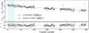 |
Fig. 1 Measurements of mid-transit times from 206Kepler transits. The green filled circles are our selection of 21 low-χ2 transits. The line represents a first-order polynomial fit to the error-weighted measurements. The lower panel shows the residuals with outliers cut-off; the variations are primarily caused by deformations of the transit due to starspots. The shaded area contains the transits that previously have been analyzed by Sanchis-Ojeda & Winn (2011). See Sects. 2.1 and 3.1 for detailed explanations. |
Reference and revised ephemeris.
2.2. Secondary eclipse
Next we use our updated ephemeris to phase-fold the light curve and search for the secondary transit of HAT-P-11 b. We define the phase p as 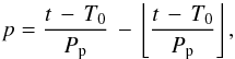 (1)where the brackets around the second term represent the floor function. Since the orbit is not circular, the secondary transit is not necessarily at phase 0.5. Using the known planetary orbit elements (Winn et al. 2010), we estimate the duration of the secondary transit to be at least 0.024 in phase. While in principle also the timing can be derived from the orbit elements, we first carry out a search for the secondary transit pretending ignorance of the timing information.
In particular, we assume a series of 200 hypothetical mid-transit phases between p = 0.25 and p = 0.75 with a phase spacing of 0.0025. For each of the 200 mid-transit phases, we normalize all observed (hypothetical) transits by dividing by a first-order polynomial fit to the adjacent continuum and superimpose the phase-folded, normalized light curves. To avoid including the secondary transit in the continuum normalization, we define a continuum range of [p−0.025,p−0.013] and [p + 0.013,p + 0.025] around mid-transit phase, which leaves some margin for a secondary transit duration of up to 0.026. Again, transits with insufficient continuum coverage were rejected. The superposed, normalized light curves were rebinned to a binsize of 0.001 in phase, which yields approximately 1500 data points per bin. To estimate the error of the rebinned data points, we calculate the standard deviation of points in all 200 hypothetical secondary transits, resulting in a value of σreb = 3.72 × 10⁻⁶.
For each hypothetical transit we then calculate the mean of the continuum points μc and the mean of in-transit points μt. For those choices of mid-transit phase that do not correspond to a real physical signal, the derived secondary transit depth μc−μt will assume stochastic values determined by the characteristics of the light curve. However, any detectable transit-like signal should be associated with a significant positive excursion. In Fig. 2 (upper panel) we plot the derived μc−μt values as a function of the assumed mid-transit orbital phase. We find two mid-transit phases for which the depth strongly deviates toward the positive side of the distribution. The highest positive deviation is found at about phase 0.66. Another, somewhat less pronounced peak is located at a phase of about 0.3. Both positive peaks are accompanied by negative deviations on either side; these “swings” reflect the fact that points in the phase window move from the continuum region into the transit window and back into the continuum again as the hypothetical transit mid-point advances. In fact, such a swing is expected from a persistent, transit-like feature in the light curve with its true position located close to the peak.
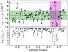 |
Fig. 2 Upper panel: mean of continuum points μc minus mean of in-transit points μt over orbital phase (see Sect. 2.2 for details). The horizontal (green) area marks the range between the 16% and 84% quantiles of the distribution of points, the gray dashed line indicates the 99.9% quantile. The position of the secondary transit of HAT-P-11 b predicted by RV measurements is given by the vertical (magenta) line; the shaded area indicates the ± σ uncertainty of the prediction. Lower panel: estimate of the significance of the measurements in the upper panel using an F-test (see Sect. 2.2 for details). |
To estimate the significance of the hypothetical transit signals presented in Fig. 2 (upper panel), we apply the ANOVA F-test (Rawlings et al. 2001). Specifically, we compare the null hypothesis of a single mean flux value in the selected continuum and transit window with the hypothesis of deviating fluxes μt and μc in the transit and continuum windows (i.e., a non-vanishing transit depth) for each of our 200 mid-transit phases. To that end, we compute the best-fit reduced χ2 values for both models, compute the F-statistic, and obtain the p-value, which we show in the lower panel of Fig. 2. The p-value gives the probability of obtaining an F-value as large or larger by chance given that the null hypothesis is true, which means that the flux is indeed constant. The largest hypothetical secondary transit depth at a phase of 0.66 is associated with a p-value of nearly 10-7, which is more than ten times smaller than for any other tested transit phase. Nonetheless, also other structures are associated with low p-values, most notably, the peak at phase ≈ 0.3. We cannot rule out that this indicates another transit-like signal potentially originating in the HAT-P-11 system; if so, we are unable to provide a reasonable explanation for its origin. At any rate, the signal at phase p ≈ 0.66 remains the deepest and most significant and, as we will see shortly, is almost certainly associated with the planetary eclipse.
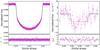 |
Fig. 3 Data of the primary (left panel) and secondary transit (right panel) overplotted by the lowest deviance solution (black line). The lower panels show the residuals. The primary data contains almost 4500 data points coming from the sample of 21 low-χ2 transits; the secondary data is rebinned to intervals of length 0.001 in phase, each containing roughly 1500 short-cadence points. |
Based on the orbital elements reported by Winn et al. (2010), we can derive the timing of the secondary transit as predicted by the radial velocity analysis; note that we shifted the argument of periastron, ω, by 180° to represent the planetary rather than the stellar orbit (e.g., Deming et al. 2011). The vertical line in Fig. 2 (upper panel) gives the expected phasing of the secondary transit and the magenta-colored, vertical area shows the range of uncertainty considering the errors in the eccentricity and the argument of periastron reported by Winn et al. (2010).
Figure 2 clearly demonstrates that the location of the deepest transit-like signal detected in our search is entirely consistent with the secondary transit phasing expected from the orbital elements reported by Winn et al. (2010). Therefore, we identify this feature with the secondary transit signature of HAT-P-11 b. Our analysis yields an approximate mid-transit phase of p = 0.659 for the secondary transit. We use this together with the previously defined continuum range to normalize the data and display the resulting rebinned light curve of the secondary eclipse in Fig. 3 (right panel).
2.3. Eccentric orbit
To carry out a more detailed analysis of the transits, we now model both the primary and secondary transit simultaneously. The primary transit modeling is based on the 21 transits with weak starspot contamination identified in Sect. 2.1, which we phase-folded with our orbital period. Each transit is again normalized individually according to the procedure described in Sect. 2.1. For the secondary transit, the preliminary mid-transit time, binsize, and continuum are defined according to Sect. 2.2, and we adopt σreb as error for each point of the rebinned light curve. All transit parameters, now including the eccentricity e, the argument of periastron ω, and the time of periastron passage τ are varied and their posterior distributions are sampled by the MCMC algorithm.
We model the secondary transit using a “conventional” primary transit model with no stellar limb darkening and introduce an additional parameter for the brightness contrast between the stellar and planetary disk. With the brightness contrast described by the parameter f3 and a first-order polynomial parameterization of the continuum with offset co and gradient cl, the observed flux f of the secondary transit light curve is modeled by the function  (2)where df(t) is the relative decrease in flux calculated by the geometric transit model (Mandel & Agol 2002). All other parameters are coupled to the values of the primary transit so that both transits are modeled based on the same set of orbital elements. For technical reasons, we applied a shift of 180° to the argument of periastron, which effectively reflects the orbit through the origin, allowing to model the secondary transit as a primary transit.
In a first step, we use uniform priors in the modeling to derive estimates based solely on the Kepler photometry. In order to incorporate prior knowledge, we then repeat the MCMC sampling including Gaussian priors on Rp/Rs, i, a/Rs, e, and ω based on the values reported by Winn et al. (2010). The prior information comprises results derived from RV measurements, which usually constrain the eccentricity and argument of periastron better than photometry alone. The results are given in Table 2, also containing the lowest deviance solution which is plotted in Fig. 3 along with the data.
Model parameters of HAT-P-11 b.
3. Results
3.1. Ephemeris
From our modeling presented in Sect. 2.1 we can derive estimates for the mid-transit times  (3)for all 206 considered primary transits in the Kepler light curve; here, T1 and T4 denote the start of ingress and the end of egress. We compare the thus derived mid-transit times to the ephemeris Tref and Pref (Table 1) given by Sanchis-Ojeda & Winn (2011) by calculating the offset according to
  (4)where E is the epoch with respect to the first Kepler transit (E = 0). The resulting offsets are given in Fig. 1.
At early epochs, there is a clear offset of about 2 min between our measurements and the ephemeris given by Sanchis-Ojeda & Winn (2011), which we speculate results from a different definition of their reference time, Tref, and our mid-transit time. As the epoch advances, the offset decreases, indicating that the orbital period is slightly shorter than the reference period reported by Sanchis-Ojeda & Winn (2011).
We calculate updated ephemeris by fitting the measurements with a first-order polynomial (linear function) using MCMC sampling. The straight line in Fig. 1 indicates the lowest deviance solution and the parameter estimates are given in Table 1. Repeating the fit with a Nelder-Mead minimization algorithm (Nelder & Mead 1965) produces results numerically identical to the MCMC lowest deviance solutions. We define T0 as the expected mid-transit time at epoch zero, which equals the median value of the offset in our polynomial fit. While the derived orbital period is somewhat lower than that reported by Sanchis-Ojeda & Winn (2011), who studied only the first 28 transits (shaded area of Fig. 1), it is still consistent within their 2σ uncertainty. Extrapolating our ephemeris backward to the epoch corresponding to the central transit time given by Bakos et al. (2010), we obtain an offset of 1.06 s, which is entirely consistent with their stated uncertainty of 28 s.
Figure 1 also shows the residuals (O−C) in the lower panel. Clearly, the statistical errors of the individual transit mid-times are smaller than the width of their distribution. Since the shift in individual mid-transit times also depends on the deformation of the transit profile by spot-crossing events (Ioannidis et al. 2016), we attribute this discrepancy to the effects of stellar activity.
Although our measurements do pin down the statistical uncertainty on T0 to less than one second and to less than 10-2 s for the orbital period, one should keep in mind that these statistical estimates might be somewhat optimistic in view of the pronounced transit deformations caused by starspot occultations. With 206 measurements, however, we expect that the orbital period should only weakly be affected by the spot crossings, even if their positions are not statistically distributed in the transits as found by Sanchis-Ojeda & Winn (2011) and Béky et al. (2014). However, with spot features repeating at similar locations, which might be the case for HAT-P-11 b during all of the Kepler observations, T0 could be systematically shifted. To obtain some estimate of the possible magnitude of that effect, we check how much our reference time shifts (keeping Pp fixed) if we only fit the 21 low-χ2 transits (filled, green circles in Fig. 1). This results in an offset of about 3.5 s, which is roughly ten times the statistical uncertainty of T0 and probably represents a more realistic estimate of the true uncertainty.
3.2. Primary transit modeling
3.2.1. Planetary radius
One of the key results of photometric transit modeling is the planet-to-star radius ratio. Deming et al. (2011) report stellar and planetary radii of Rs = (0.683 ± 0.009) R⊙ and Rp = (4.39 ± 0.06) R⊕. In their analysis, they estimate that uneclipsed starspots, not prominently showing as crossing events during the transit, make the planetary radius appear larger by 1.76%, reducing the derived physical planetary radius to a value of (4.31 ± 0.06) R⊕.
Adopting their stellar radius, and relying on our measurement of Rp/Rs (Table 2) from our sample of 21 low-χ2 transits, we determine a planetary radius of (4.36 ± 0.06) R⊕. As a result of our normalization procedure (see Sect. 2.1), we expect the effects of unocculted spots on our planet-to-star radius ratio to be small, and we do not apply Deming et al.’s correction factor. Our result for the planetary radius is slightly larger, but still consistent with the spot-corrected value reported by Deming et al. (2011).
A systematic error in the planetary radius derived in our analysis may result from persistent and symmetrical spot coverage not showing in the rotational modulation (e.g., a long-lived polar spot), which can neither be excluded by our analysis nor would it be accounted for by our normalization approach. While such a configuration would lead to an overestimation of the radius, we expect that our sample of low-χ2 transits is also influenced by spot-crossing features at some level. In fact, the distribution of residuals with respect to the primary transit model (Fig. 3, lower left panel) is symmetrical. However, a reduced χ2 value of 2.4 resulting from the primary transit model, leads us to the assumption that the error of individual in-transit data points is underestimated and is larger than in the adjacent continuum, from where we obtain the error estimate. Additionally, a likely signature of a spot-crossing feature is visible at orbital phase ≈ 0.005. This indicates that additional noise sources affect the in-transit light curve, most likely including signatures of small, unresolved spot-crossing events. Such signatures lead to an underestimation of the radius ratio, and thus counteracts the effects of persistent, unocculted spots. Therefore, we adopt Rp = (4.36 ± 0.06) R⊕ as our best estimate, but caution that the uncertainty is likely underestimated because of the presence of unaccounted for systematic errors.
3.2.2. Limb darkening
In general, stellar limb-darkening (LD) is considered a nuisance parameter in transit modeling which has to be accounted for when deriving planetary parameters. However, space-based (short-cadence) photometry of exoplanetary transits, as provided for example by Kepler or CoRoT, offers one of only very few possibilities to directly measure the LD of stellar disks with high precision. There is an ongoing discussion on which limb-darkening “laws” should be used and whether one achieves more reliable results when keeping the LD coefficients fixed to theoretically predicted values or not (e.g., Howarth 2011; Csizmadia et al. 2013; Müller et al. 2013; Espinoza & Jordán 2015).
We applied a quadratic limb-darkening law and left the LD coefficients free in the MCMC sampling resulting in  and
and  for the linear and quadratic coefficient, respectively. Claret et al. (2012) determine theoretical values from PHOENIX models for the Kepler bandpass using two different fitting approaches which yield parameter estimates between 0.6937 and 0.7076 for u1 and 0.0382 and 0.0772 for u2 (Teff = 4800 K and log g = 4.5). For the latter, our result lies well between the two predictions; considering its absolute value, the linear coefficient does not strongly deviate from the predicted range, although within its uncertainties it lies significantly below the theoretical values. The LD of an highly active star as HAT-P-11 is likely influenced by cool and hot regions on its surface which is not considered in the theoretical predictions. Also our determined values for u1 and u2 are probably affected by starspots to some degree. Considering these systematic uncertainties, we conclude that our LD values agree reasonably with the theoretical expectation.
3.3. Secondary eclipse and orbital eccentricity
Figure 3 presents the data of primary and secondary transit as well as the lowest deviance model of the combined fit. Table 2 contains the lowest deviance values, the median values of the posterior distributions for a model with uniform priors, and another model with the results of Winn et al. (2010) incorporated as Gaussian priors. The parameter estimates from both models agree within their 68% credibility intervals, which also cover the lowest deviance solution. This indicates that there is no strong influence of the prior information on the posterior distribution. Actually, we find the width of the Gaussian priors to be much broader than the posterior credibility intervals (e.g., almost 100 times larger for e and about 50 times larger for ω) and conclude that the likelihood entirely dominates the posterior and, thus, both solutions become virtually identical. Nonetheless, as the estimated values including the prior information comprehensively represent the available knowledge, we prefer this solution and base our following calculations and discussions on these values.
For the secondary transit model, we obtain a reduced χ2 value of 0.9 (Fig. 3, lower right panel), indicating that errors may be slightly overestimated here. In fact, the evolution of the in-transit flux of the secondary eclipse seems to show a positive gradient with the minimum flux reached shortly after ingress. If this evolution should be real, we argue that it can hardly be related to the secondary planetary eclipse, because during its totality phase the planet is behind the star and not visible. Recalling that the shown data set is composed of 208 individually normalized light curves, we argue that this structure is likely an artifact.
We calculate the Poisson noise σlimit of each bin of the secondary transit data for comparison to our estimated uncertainty of σreb = 3.72 × 10⁻⁶. Using an average count rate of 2.7 × 10⁶ e−/s (electrons per second) for the Kepler light curve, the length of each rebinned time interval (421.6 s), and the number of averaged secondary transits (208), we derive σlimit = 2 × 10⁻⁶. Our estimated noise is only about a factor two larger than the theoretical limit.
According to our modeling, the depth ds of the secondary transit is  ppm, which corresponds to a 5.5σ detection of a decline in flux. Therefore, we argue that it is extremely unlikely to be a statistical artifact, especially because its position was correctly predicted by independent measurements of the orbital elements. Nonetheless, the transit signal remains weak compared to the uncertainty of individual data points. Angerhausen et al. (2015) searched for the secondary eclipse concluding that the depth of the secondary transit has to be less than 147 ppm, which is of course consistent with our results.
3.3.1. Secondary transit duration
The duration of the secondary transit is directly related to the orbital elements. Table 2 provides calculations of the impact parameters b and bsec of the primary and secondary transit as well as their durations T14 and T14,sec. The values of impact parameter and duration are determined using (5)and
  (6)Due to our definition of ω relating to the planet, Eqs. (5) and (6) refer to the secondary eclipse for the plus sign and to the primary eclipse for the minus sign wherever ± is given; naturally, shifting ω by 180° produces the same sign change.
To calculate the time between primary and secondary eclipse, we use the equation  (7)which yields the time between two points t1 and t2 of a planet on an eccentric orbit; here ν denotes the true anomaly which is a function of time. For the primary and secondary transits we use ν1 = −π/ 2−ω = νp and ν2 = π/ 2−ω = νs and numerically solve the equation for our MCMC chains of the eccentricity and the argument of periastron, thus obtaining an uncertainty estimate for Δts−p/Pp with a negligible numerical error. We note that the commonly used expression to derive the separation in orbital phase between primary and secondary transit
  (8)which is the first-order Taylor series expansion of Eq. (7) at e = 0, should not be used in this case3. HAT-P-11 b’s large eccentricity and our small uncertainties lead to a result that deviates by more than 2σ from Eq. (7).
The results derived from Eqs. (5)–(7) are fully consistent with the orbit of the planet. During primary transit the planet is closer to the star and moves faster, leading to a smaller impact parameter and shorter transit duration than for the secondary eclipse. T14,sec is almost 24 min longer than the primary transit with only a small error of roughly 20 s. The mid-time of the secondary eclipse occurs 3.22 days after the primary eclipse, leading to a separation in time almost twice as long as that between secondary and primary (1.67 days); the uncertainties for Δts−p lie between two and four minutes.
3.3.2. Light travel time effect
When star and planet move around their common center of mass, the planet is physically more distant from the observer during secondary eclipse than during primary eclipse. Thus, that part of the light coming from the planet just before and after the secondary eclipse must have traveled longer to reach the observer. Consequently, the secondary transit is observed later than it actually occurs geometrically. In particular, it is delayed by  (9)where c is the speed of light, and
  and mp = (0.081 ± 0.009) MJ are the masses of star and planet taken from Bakos et al. (2010).
Using Eq. (9), we estimate the amplitude of the light travel time effect to be Δttravel ≈ 44 s for our orbital solution. Given a temporal binning of seven minutes for the secondary eclipse data and an uncertainty of two to four minutes in our mid-transit time for the secondary, we estimate that considering Δttravel in our results would change the eccentricity and the argument of periastron by only about a third of their uncertainty interval, slightly moving e to smaller and ω to larger values. Thus light travel time effects play only a minor role in our modeling.
3.4. Albedo and equilibrium temperature
The measured depth of the secondary eclipse  (10)provides an opportunity to determine the albedo and the equilibrium temperature of HAT-P-11 b. The secondary eclipse depth is related to the planetary geometric albedo Ag through
  (11)where we use the distance rsec of the planet from the star during secondary eclipse instead of the semi-major axis a to account for the eccentric orbit.
A potentially confounding factor in relating the secondary eclipse depth to the geometric albedo is a possible contribution of thermal emission to the eclipse depth. The fraction of the planetary thermal flux fthermal in the Kepler bandpass, which covers wavelengths between λ1 ≈ 4000 Å and λ2 ≈ 9000 Å, can be estimated by  (12)from Han et al. (2014), where Teq is the planetary equilibrium temperature, Bλ is the blackbody intensity, and σSB is the Stefan-Boltzmann constant. In the following calculations we show that this contribution is negligible.
The planetary equilibrium temperature is related to the stellar effective temperature Ts, the Bond albedo Ab, and the redistribution factor fredist, characterizing the energy redistribution within the planetary atmosphere, as  (13)where the factor Rs/r(t) accounts for the distance of the planet from the bright stellar surface. An energy redistribution factor fredist of 2/3 accounts for a non-uniform distribution of flux over the surface of the planet with the substellar point receiving the most intense irradiation; fredist = 1/2 represent the case when all incoming flux is reradiated isotropically from each point of the irradiated hemisphere (see Hansen 2008). A uniform distribution of flux over the entire surface of the planet would be accounted for by fredist = 1/4.
Following Han et al. (2014), we assume that geometric and Bond albedo are related via Ab = 3/2 Ag. Due to the non-vanishing eccentricity, the planetary equilibrium temperature becomes a function of the time-dependent orbital distance r(t) of the planet, which we use in Eq. (13). In this expression, any dynamical effects in the planetary atmosphere are of course ignored and instantaneous adjustment of the atmosphere to the received radiative input is assumed.
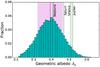 |
Fig. 4 Distribution of the geometric albedo Ag of HAT-P-11 b (histogram). The (magenta) line and area indicate the median and 68% credibility interval. The visual geometric albedos of the Solar System giant planets are given for comparison. |
Adopting Ts = (4780 ± 50) K (Bakos et al. 2010) as the effective stellar temperature of HAT-P-11, we calculate the geometric albedo Ag and planetary effective temperature Teq based on the traces of our MCMC sampling with priors. In Fig. 4 we present the marginal distribution for the geometric albedo Ag, including the visual geometric albedos of the Solar System giant planets4 for reference.
We ignore the thermal correction to Ag because fthermal is only <2 × 10⁻⁴ for fredist = 2/3, and becomes even smaller for fredist = 1/2, which is negligible. Even if we insert the highest Teq of the planet on its orbit, fthermal is still insignificant. Although we would have to measure the phase curve of HAT-P-11 b to derive reliable estimates of the brightness of the planet’s night side, the low estimate for the fraction of thermal flux indicates that the night side of HAT-P-11 b remains virtually invisible to Kepler, which records only the reflected stellar flux.
Figure 4 shows that Neptune’s albedo lies well inside the credibility interval of Ag = 0.39 ± 0.07, close to the expectation value. The albedo of Saturn is only slightly beyond the 84% quantile and those of Uranus and Jupiter are about 2σ off. The planet HAT-P-11 b has roughly the size of Neptune and also a similar albedo, which might indicate a further similarity between these two bodies, even though their orbits are very different.
In recent years several albedos of exoplanets have been measured using Kepler data. Angerhausen et al. (2015) present a comprehensive study of 20 confirmed Kepler planets. They detect secondary eclipses in 16 cases and derive geometric albedos which are all smaller than our result for HAT-P-11 b, although the albedo of Kepler-44 b (KOI-204) has a relatively large uncertainty. Their largest value is Ag = 0.32 ± 0.03 for Kepler-7 b (KOI-97), a low-density planet with a mass of Mp = 0.43 MJ and a radius of Rp = 1.48 RJ (Latham et al. 2010). Esteves et al. (2015) study a sample of 14Kepler planets reporting that 11 objects have albedos smaller than 0.25. They argue that from the three cases with larger albedos probably only the result of Kepler-10 b with Ag = 0.58 ± 0.25 is reliable; interestingly, Kepler-10 b (Batalha et al. 2011) is a rather special planet in their sample with a very short period, small radius, and rocky composition, probably not having an atmosphere. Furthermore, Sheets & Deming (2014) published an analysis of 31 sub-Saturn Kepler candidate planets and determine the average albedo of the sample. Excluding Kepler-10 b from their sample, they find a geometric albedo of Ag = 0.22 ± 0.06, whereas Kepler-10 b represents an outlier with Ag = 0.60 ± 0.09. It seems that HAT-P-11 b lies at the upper end of geometric albedos measured for exo-planets with the radius of Neptune or larger; it maybe even occupies a niche between these planets and super-Earths such as Kepler-10 b with rocky compositions and thin or no atmospheres. However, Kepler-10 b might also just represent a statistical outlier; after all the geometric albedos of Solar System rocky planets are small, except for Venus with its dense atmosphere. Finally, we note that in contrast to HAT-P-11 b none of the exoplanets in the samples of Sheets & Deming (2014), Esteves et al. (2015), and Angerhausen et al. (2015) shows a significant eccentricity. Whether this has an effect on the albedo, however, remains to be determined.
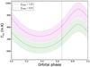 |
Fig. 5 Equilibrium temperature Teq of HAT-P-11 b over orbital phase for a redistribution factor fredist of 1/2 and 2/3. The vertical line is the position of the secondary eclipse. The shaded areas indicate the 68% credibility intervals. |
We show the derived equilibrium temperature of HAT-P-11 b in Fig. 5; the colored margins represent a full error propagation for all input parameters to Eq. (13), with the exception of r(t), which has a negligible contribution. The dominating uncertainty comes from the stellar effective temperature Ts. We emphasize that Teq represents an estimate for the brightness temperature of HAT-P-11 b’s day side, which is seen close to secondary eclipse. The temperature on the night side depends crucially on the energy transport mechanisms in the planet’s atmosphere and the rotation of the planet, both of which remain unknown. Thus, Fig. 5 should not be confused with the “brightness” of the visible hemisphere of HAT-P-11 b over its orbital phase.
Teq is a function of time and highest when the planet is closest to the star near its periastron. Because at that time the planet also moves fastest, this “hot phase” of the planet lasts only for a relatively small period of time compared to the entire orbital period. Thus, on the far side of the orbit the equilibrium temperatures are lowest and the temperature gradient is smallest as well. Since we do not know the redistribution of heat in the planetary atmosphere, we present the temperature for both fredist = 2/3 and fredist = 1/2. As expected from Eq. (13), the values for fredist = 2/3 are higher. Both models differ the least (ΔT ≈ 100 K) when the planet is coolest, but the temperature difference rises to almost 130 K during periastron. The median temperature of the planet for fredist = 1/2 is 680 K, with a maximum temperature difference of 200 K over one orbit; for fredist = 2/3 the corresponding values are 790 K and 230 K. Even for the latter high-temperature solution, HAT-P-11 b remains cooler than the day side of Mercury over half of its orbital period.
4. Summary
We present an in-depth transit analysis of all available Kepler short-cadence data of the planetary system HAT-P-11. First, we derived updated planetary ephemeris; using our revised reference epoch T0 and orbital period Pp, we were able to report the first detection of the secondary eclipse of HAT-P-11 b based on the phase-folded Kepler light curve. Second, we carried out simultaneous primary and secondary transit modeling. Here, we specifically selected a sample of primary transit light curves which are only weakly affected by spot-crossing signatures. The orbital elements and planetary parameters determined from our modeling are consistent with previous estimates for the primary transit, although we present significantly reduced statistical uncertainties for most of the parameters.
In combination with the secondary eclipse, we pin down the eccentric orbit of HAT-P-11 b to a much higher precision than previously determined using RV measurements; the phasing of the secondary eclipse yields an orbital eccentricity of  . We determine a secondary eclipse depth of ppm, which translates into a geometric planetary albedo of 0.39 ± 0.07 for HAT-P-11 b. Among the Solar System giant planets, this is best consistent with Neptune; however, the uncertainty remains too large to reliably rule out consistency with the albedos of the other giants. Whether the similarity between HAT-P-11 b and Neptune reaches beyond their sizes and albedos has to be determined by future studies.
Due to HAT-P-11 b’s non-circular orbit, the planetary equilibrium temperature changes with phase. We determine temperatures between 630 K and 950 K, which depend on assumptions on the atmospheric energy redistribution; no detailed modeling of the atmosphere has been attempted here. While our analysis does not provide direct information on the night side brightness of HAT-P-11 b, we estimate the fraction of planetary thermal flux in the Kepler bandpass to be small. In combination with the strong rotational modulation of the light curve due to starspots, this makes the study of the phase curve of this planet in this data set highly challenging. However, future observations at infrared wavelengths, where the impact of stellar activity is weaker (e.g., by SOFIA or JWST), might allow to resolve the planetary phase curve and provide further insight into the physics of this intriguing planetary system.
The subtraction from unity on the right-hand side of Eq. (8) is again a result of our shift of ω by π.
Acknowledgments
All of the Kepler data presented in this paper were obtained from the Mikulski Archive for Space Telescopes (MAST). STScI is operated by the Association of Universities for Research in Astronomy, Inc., under NASA contract NAS5-26555. Support for MAST for non-HST data is provided by the NASA Office of Space Science via grant NNX09AF08G and by other grants and contracts. This paper includes data collected by the Kepler mission. Funding for the Kepler mission is provided by the NASA Science Mission directorate. This research has made use of the SIMBAD database, operated at CDS, Strasbourg, France (Wenger et al. 2000). This research has made use of the Exoplanet Orbit Database and the Exoplanet Data Explorer at exoplanets.org (Han et al. 2014). This work made extensive use of PyAstronomy5. K.F.H. thanks the German Research Foundations (DFG) for grants under HU 2177/1-1.
References
- Angerhausen, D., DeLarme, E., & Morse, J. A. 2015, PASP, 127, 1113 [NASA ADS] [CrossRef] [Google Scholar]
- Bakos, G. Á., Lázár, J., Papp, I., Sári, P., & Green, E. M. 2002, PASP, 114, 974 [NASA ADS] [CrossRef] [Google Scholar]
- Bakos, G., Noyes, R. W., Kovács, G., et al. 2004, PASP, 116, 266 [NASA ADS] [CrossRef] [Google Scholar]
- Bakos, G. Á., Torres, G., Pál, A., et al. 2010, ApJ, 710, 1724 [NASA ADS] [CrossRef] [Google Scholar]
- Batalha, N. M., Borucki, W. J., Bryson, S. T., et al. 2011, ApJ, 729, 27 [NASA ADS] [CrossRef] [Google Scholar]
- Béky, B., Holman, M. J., Kipping, D. M., & Noyes, R. W. 2014, ApJ, 788, 1 [NASA ADS] [CrossRef] [Google Scholar]
- Borucki, W. J., Koch, D., Basri, G., et al. 2010, Science, 327, 977 [NASA ADS] [CrossRef] [PubMed] [Google Scholar]
- Claret, A., Hauschildt, P. H., & Witte, S. 2012, A&A, 546, A14 [NASA ADS] [CrossRef] [EDP Sciences] [Google Scholar]
- Csizmadia, S., Pasternacki, T., Dreyer, C., et al. 2013, A&A, 549, A9 [NASA ADS] [CrossRef] [EDP Sciences] [Google Scholar]
- Czesla, S., Huber, K. F., Wolter, U., Schröter, S., & Schmitt, J. H. M. M. 2009, A&A, 505, 1277 [NASA ADS] [CrossRef] [EDP Sciences] [Google Scholar]
- Deming, D., Sada, P. V., Jackson, B., et al. 2011, ApJ, 740, 33 [NASA ADS] [CrossRef] [Google Scholar]
- Espinoza, N., & Jordán, A. 2015, MNRAS, 450, 1879 [NASA ADS] [CrossRef] [Google Scholar]
- Esteves, L. J., De Mooij, E. J. W., & Jayawardhana, R. 2015, ApJ, 804, 150 [NASA ADS] [CrossRef] [Google Scholar]
- Han, E., Wang, S. X., Wright, J. T., et al. 2014, PASP, 126, 827 [NASA ADS] [CrossRef] [Google Scholar]
- Hansen, B. M. S. 2008, ApJS, 179, 484 [NASA ADS] [CrossRef] [Google Scholar]
- Hirano, T., Narita, N., Shporer, A., et al. 2011, PASJ, 63, 531 [NASA ADS] [Google Scholar]
- Howarth, I. D. 2011, MNRAS, 418, 1165 [NASA ADS] [CrossRef] [Google Scholar]
- Ioannidis, P., Huber, K. F., & Schmitt, J. H. M. M. 2016, A&A, 585, A72 [NASA ADS] [CrossRef] [EDP Sciences] [Google Scholar]
- Latham, D. W., Borucki, W. J., Koch, D. G., et al. 2010, ApJ, 713, L140 [NASA ADS] [CrossRef] [Google Scholar]
- Mandel, K., & Agol, E. 2002, ApJ, 580, L171 [NASA ADS] [CrossRef] [Google Scholar]
- McLaughlin, D. B. 1924, ApJ, 60, 22 [NASA ADS] [CrossRef] [Google Scholar]
- Müller, H. M., Huber, K. F., Czesla, S., Wolter, U., & Schmitt, J. H. M. M. 2013, A&A, 560, A112 [NASA ADS] [CrossRef] [EDP Sciences] [Google Scholar]
- Nelder, J. A., & Mead, R. 1965, The Comput. J., 7, 308 [CrossRef] [Google Scholar]
- Rawlings, J., Pantula, S., & Dickey, D. 2001, Applied Regression Analysis: A Research Tool, Springer Texts in Statistics (New York: Springer) [Google Scholar]
- Rossiter, R. A. 1924, ApJ, 60, 22 [NASA ADS] [CrossRef] [Google Scholar]
- Sanchis-Ojeda, R., & Winn, J. N. 2011, ApJ, 743, 61 [NASA ADS] [CrossRef] [Google Scholar]
- Sheets, H. A., & Deming, D. 2014, ApJ, 794, 133 [NASA ADS] [CrossRef] [Google Scholar]
- Southworth, J. 2011, MNRAS, 417, 2166 [NASA ADS] [CrossRef] [Google Scholar]
- Vogt, S. S., Allen, S. L., Bigelow, B. C., et al. 1994, in Instrumentation in Astronomy VIII, eds. D. L. Crawford, & E. R. Craine, Proc. SPIE, 2198, 362 [Google Scholar]
- Wenger, M., Ochsenbein, F., Egret, D., et al. 2000, A&AS, 143, 9 [NASA ADS] [CrossRef] [EDP Sciences] [Google Scholar]
- Winn, J. N., Johnson, J. A., Howard, A. W., et al. 2010, ApJ, 723, L223 [NASA ADS] [CrossRef] [Google Scholar]
All Tables
All Figures
|
Fig. 1 Measurements of mid-transit times from 206Kepler transits. The green filled circles are our selection of 21 low-χ2 transits. The line represents a first-order polynomial fit to the error-weighted measurements. The lower panel shows the residuals with outliers cut-off; the variations are primarily caused by deformations of the transit due to starspots. The shaded area contains the transits that previously have been analyzed by Sanchis-Ojeda & Winn (2011). See Sects. 2.1 and 3.1 for detailed explanations. |
| In the text | |
|
Fig. 2 Upper panel: mean of continuum points μc minus mean of in-transit points μt over orbital phase (see Sect. 2.2 for details). The horizontal (green) area marks the range between the 16% and 84% quantiles of the distribution of points, the gray dashed line indicates the 99.9% quantile. The position of the secondary transit of HAT-P-11 b predicted by RV measurements is given by the vertical (magenta) line; the shaded area indicates the ± σ uncertainty of the prediction. Lower panel: estimate of the significance of the measurements in the upper panel using an F-test (see Sect. 2.2 for details). |
| In the text | |
|
Fig. 3 Data of the primary (left panel) and secondary transit (right panel) overplotted by the lowest deviance solution (black line). The lower panels show the residuals. The primary data contains almost 4500 data points coming from the sample of 21 low-χ2 transits; the secondary data is rebinned to intervals of length 0.001 in phase, each containing roughly 1500 short-cadence points. |
| In the text | |
|
Fig. 4 Distribution of the geometric albedo Ag of HAT-P-11 b (histogram). The (magenta) line and area indicate the median and 68% credibility interval. The visual geometric albedos of the Solar System giant planets are given for comparison. |
| In the text | |
|
Fig. 5 Equilibrium temperature Teq of HAT-P-11 b over orbital phase for a redistribution factor fredist of 1/2 and 2/3. The vertical line is the position of the secondary eclipse. The shaded areas indicate the 68% credibility intervals. |
| In the text | |
Current usage metrics show cumulative count of Article Views (full-text article views including HTML views, PDF and ePub downloads, according to the available data) and Abstracts Views on Vision4Press platform.
Data correspond to usage on the plateform after 2015. The current usage metrics is available 48-96 hours after online publication and is updated daily on week days.
Initial download of the metrics may take a while.